Paramagnetic Nuclear Magnetic Resonance: The Toolkit

Abstract

Nuclear Magnetic Resonance (NMR) spectroscopy is the ideal tool to address the structure, reactivity and dynamics of both inorganic and biological substances. The knowledge of nuclear spin interaction and spin dynamics is increasingly consolidated, and this allows for tailoring pulse sequences. When dealing with paramagnetic systems, several decades of research have led to the development of rule-of-the-thumb criteria for optimizing the experiments, allowing for the detection of nuclei that are in very close proximity to the metal center. In turn, the observation of these systems, coupled with the development of robust and accessible quantum chemical methods, is promising to provide a link between the spectra and the structural features through the interpretation of the electronic structure. In this review, we list the challenges encountered and propose solutions for dealing with paramagnetic systems with the greatest satisfaction. In our intentions, this is a practical toolkit for optimizing acquisition and processing parameters for routine experiments aimed at detecting signals influenced by the hyperfine interaction. The implications of paramagnetic shift and line broadening are examined. With this endeavor, we wish to encourage non-expert users to consider the application of paramagnetic NMR to their systems.

1. Who

Inorganic chemistry, more specifically, coordination chemistry of transition metal ions, played an important role in the early days of NMR. When spectral resolution in NMR appeared as an insurmountable barrier preventing the study of complex molecules, small inorganic complexes showed high spectral dispersion, bringing many inorganic chemists to approach NMR [1,2,3,4,5]. A couple of decades before biochemists discovered the potentialities of high-field NMR to study macromolecular structure, dynamics and interactions [6], it was clear that the interaction between electron and nuclear spins was able to provide room temperature information on the spin state on the electronic correlation time and on the coordination geometry of molecules containing unpaired electron(s) [7,8].

2. What

In principle, each NMR experiment needs a setup procedure that takes into account relaxation properties, molecular size, number of active spins, sample concentration, aggregation conditions, temperature, sample stability, and solvent. However, real life in contemporary NMR laboratories often offers a different perspective in which, for each experiment, parameter sets optimized according to standard molecules are available to be used as a black box. Of course, no matter what has been taken as a standard, any real system will never be exactly like a test case. Therefore, this approach is, “in principle”, wrong. However, it has many positive, relevant aspects, such as saving both NMR time and personal time, giving access to the spectrometer and to non-experts, and, at the same time, protecting the fragile NMR hardware from excesses of creativity in front of the spectrometer. In an effort to provide a simple tool for the setup of basic experiments in “paramagnetic NMR”, we hereby summarize, for the more basic experiments, how starting values for acquisition parameters should be selected and on which basis to optimize them. The following cases will be discussed:

(a)

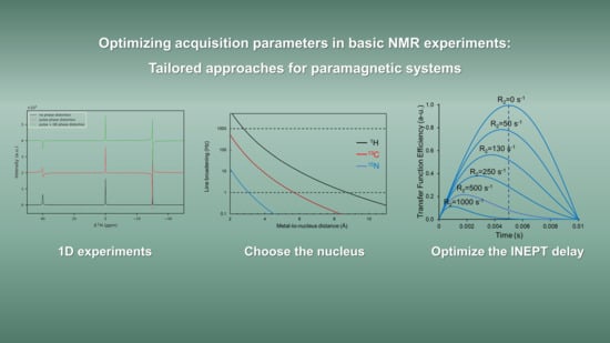
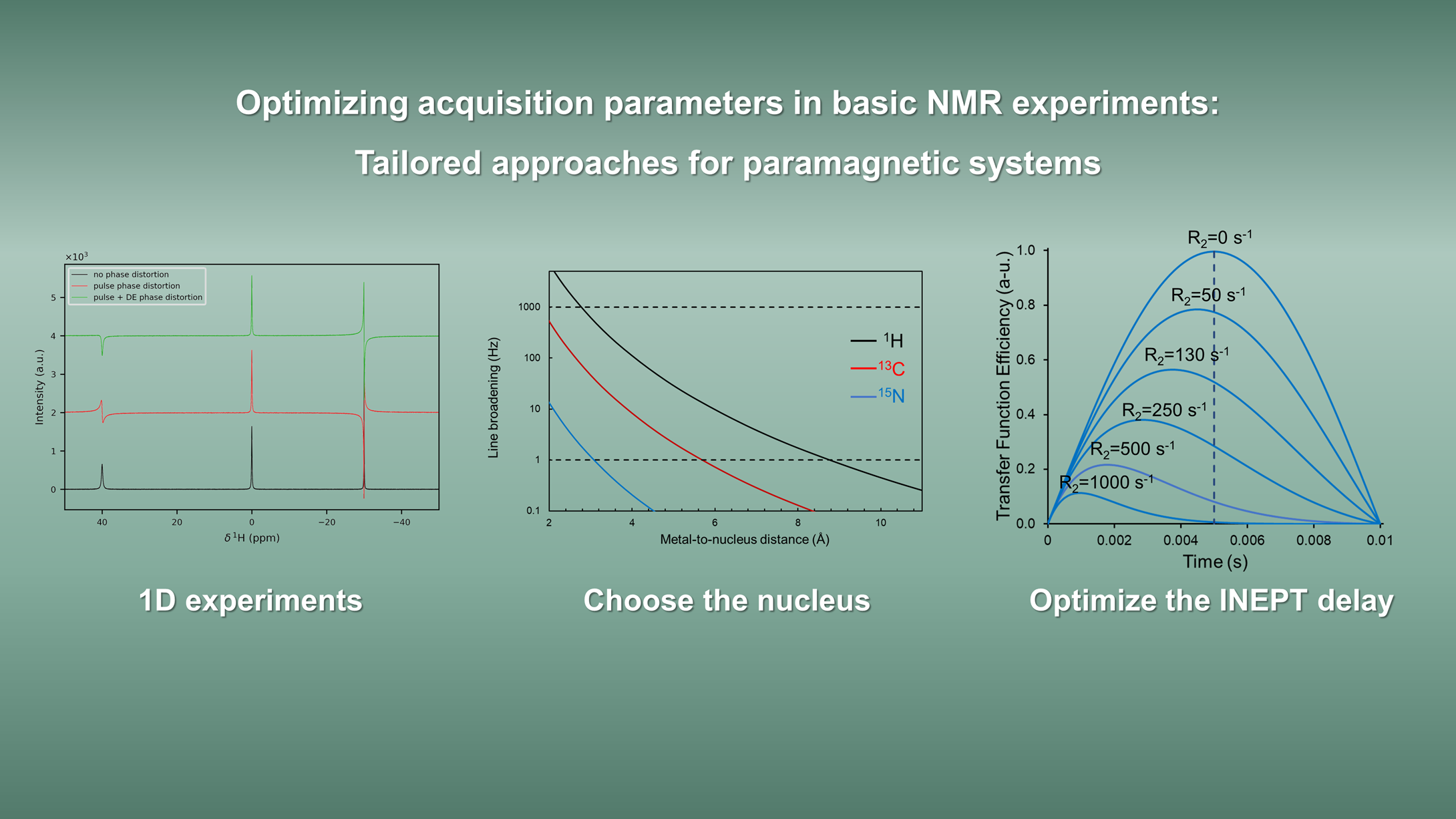
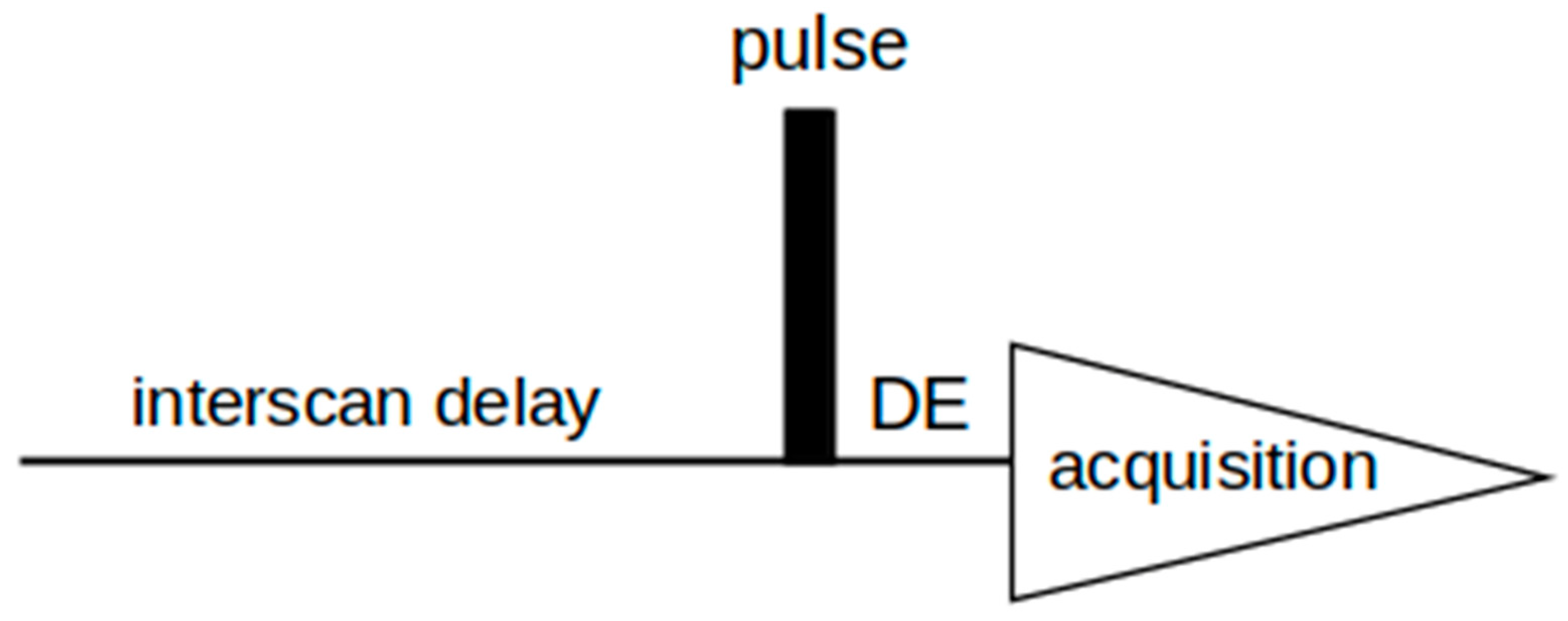
One-dimensional experiments: fast relaxation and large spectral widths

(b)

Two-dimensional homonuclear ¹H-¹H experiments

(c)

Two-dimensional heteronuclear ¹H-¹⁵N/¹H-¹³C experiments

(d)

Relaxation rate measurements

(e)

¹³C direct detected experiments

(f)

Multidimensional triple-resonance experiments

3. When/Where

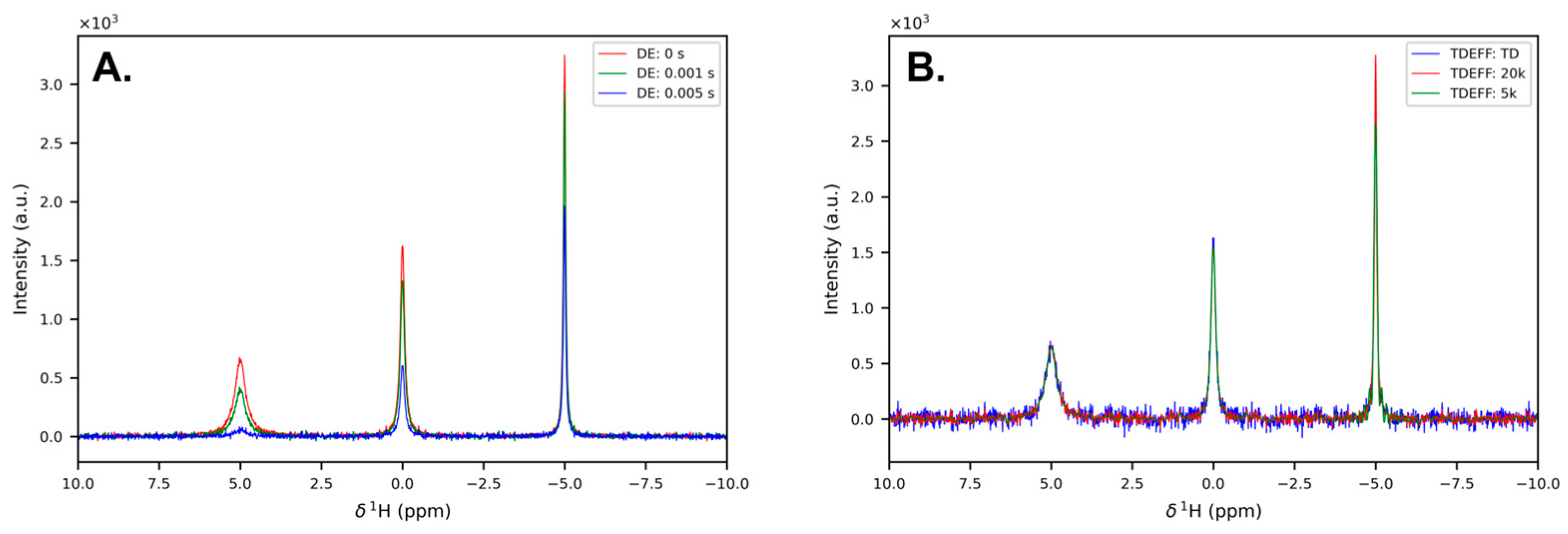
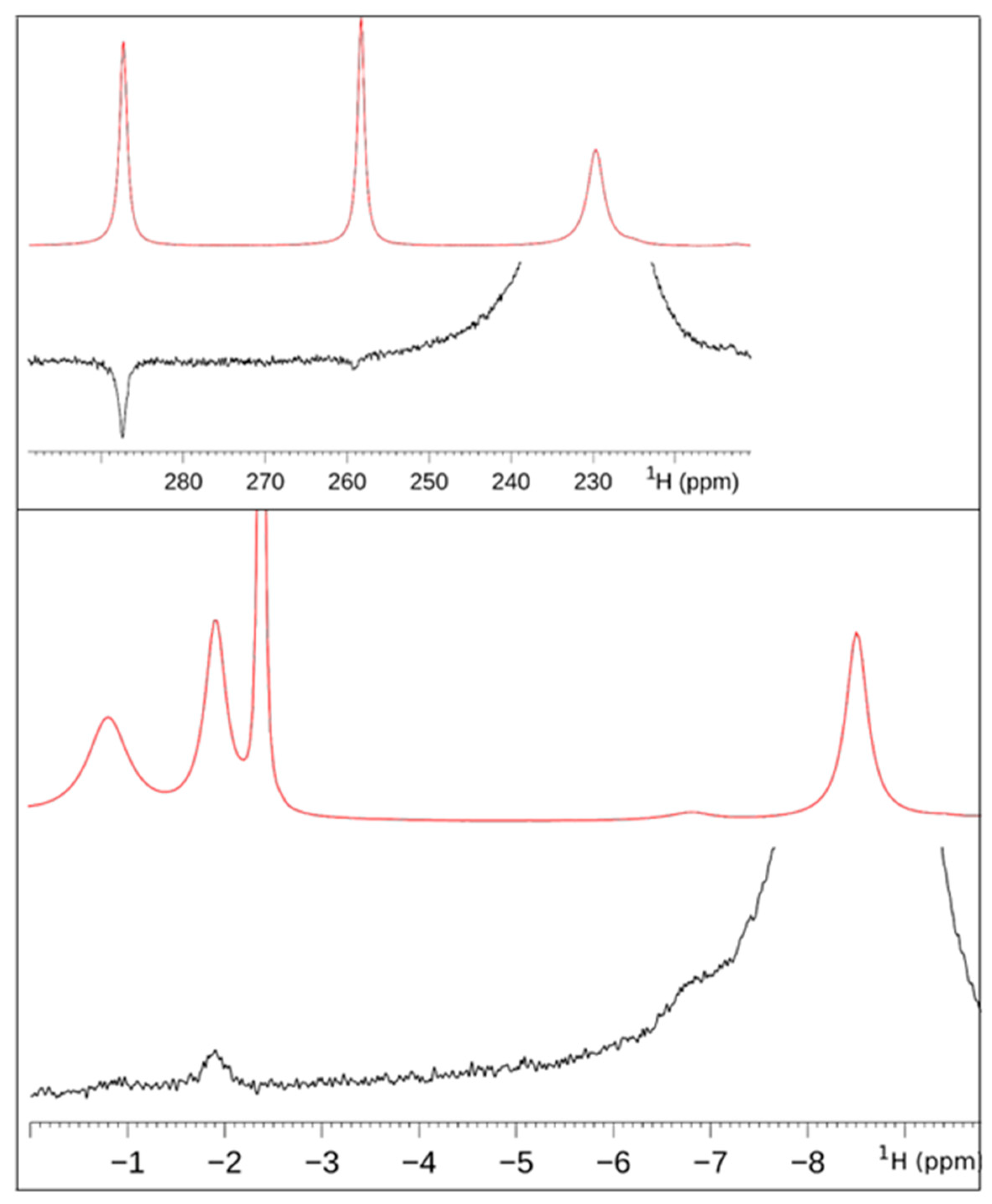
3.1. One-Dimensional Experiments: Fast Relaxation and Large Spectral Widths

As mentioned above, the presence of paramagnetic centers can produce significant shifts and broadening of the signals as a direct consequence of the hyperfine interaction between nuclear magnetic moments and the magnetic moments of unpaired electrons. Shifts and relaxation are the leading determinants in the choice of the acquisition parameters in a magnetic resonance experiment: if the lines are very broad (large transverse relaxation rate, R₂), the acquisition time can be reduced if the longitudinal relaxation is quick (large longitudinal relaxation rate, R₁), the interscan (see Figure 1) delay can be reduced, if the peaks are substantially dispersed (large shifts), short pulses with large windows and small flip angles can be used an so on (vide infra).

Of course, one does not know a priori what relaxation rates and resonance frequencies will be (which would justify not taking the spectrum and saving time for more rewarding activities). However, the ballpark for the values of these parameters, within—say—a couple of orders of magnitude for relaxation rates and a factor 2–3 for the shifts, can be guessed from the conventional wisdom about electronic structure [8]. For the vast majority of cases, we can suggest the following rule of thumb: if the electronic ground state is non-degenerate, electron relaxation is slow, nuclear relaxation is fast, and shifts tend to be small; if the electronic ground state is degenerate, electron relaxation is much faster and nuclear relaxation is slower, and shifts will probably be rather large. A concise guide is found in Figure 2 [9].

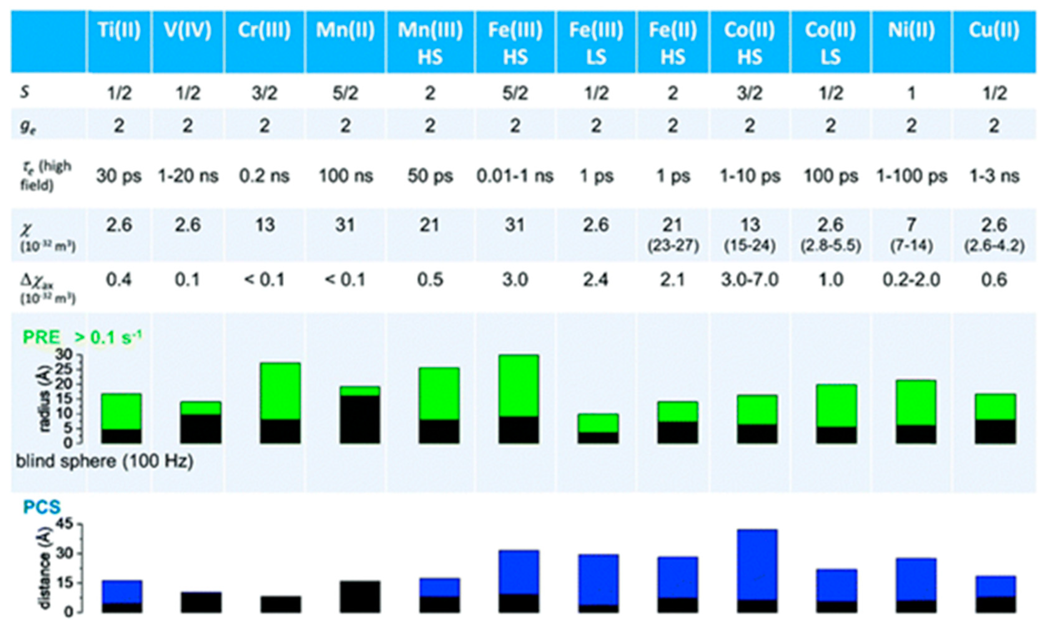
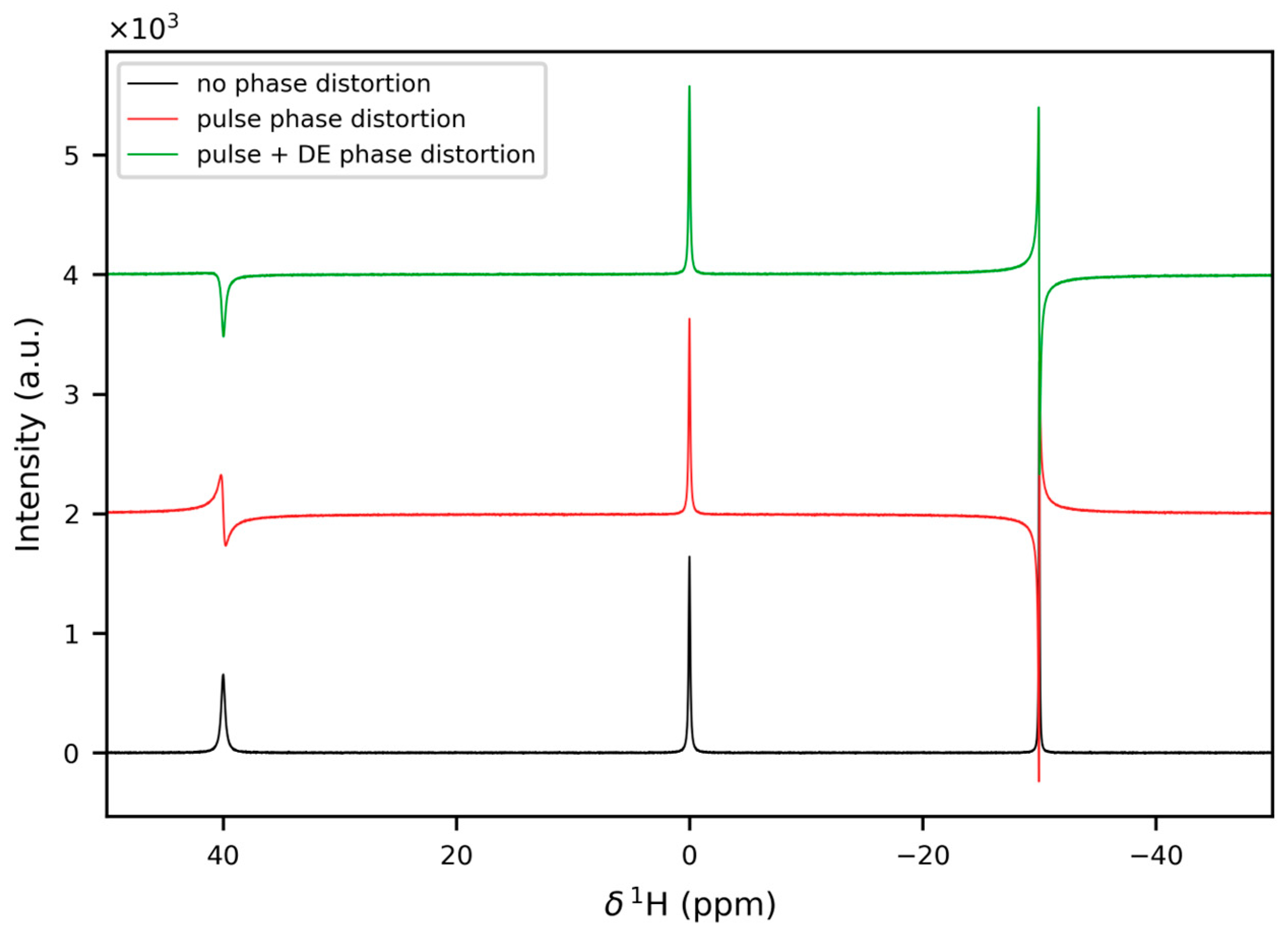
3.1.1. When Relaxation Is Fast

Dealing with paramagnetic systems quite often means dealing with short relaxation times. Sometimes, the effect is so severe as to delete some peaks: wider signals result in reduced peak heights and thus reduced signal-to-noise ratio and reduced resolution. Admittedly, this makes the expression “high resolution NMR” no longer appropriate, even at high magnetic fields. Even if all the peaks are seen, their intensities might be significantly altered. An ideal experiment would require no dead time between the end of the pulse and the start of the acquisition, but, in practice, any physical receiver requires a finite time (up to tens of microseconds, us) to reach linear response conditions after it is turned on. Therefore, if the receiver is turned on immediately after the end of the pulse, and if the dwell time (the time between two consecutive FID points during acquisition, DW) is short because of large spectral width (e.g., 2.5 us), the first several data points may have an altered intensity, which will be translated, after the Fourier Transformation (FT), into a baseline distortion. To reduce this problem, a dead time (the time between the end of the pulse and the first acquired point, DE) of the order of the time required by the receiver to achieve linearity is introduced before starting the acquisition. The DE may also be useful to avoid acoustic ringing from the probe, which may be a serious problem at low Larmor frequencies. As shown in Figure 3A, the occurrence of a delay between the end of the observation pulse and the first point digitized determines a loss of signal intensity that can be dramatic when the DE is not irrelevant compared to the transverse relaxation time (T₂) (vide infra).

Given that the information encoded in the FID decays with the T₂ of the signal of interest, acquisition times considerably longer than the longest T₂ are not recommended unless sharp or poorly resolved signals are also looked for in the spectrum. Actually, spectra containing signals with significantly different T₂ values can be processed with a varying number of points (effective number of data points used in the processing of an NMR spectrum, TDEFF) to optimize the effective acquisition times according to given T₂ values and to discriminate among different signals as shown in Figure 3B.

Every cloud has a silver lining. That of fast transverse relaxation is that it usually comes with a fast longitudinal relaxation. A fast longitudinal relaxation means that the interscan delay can be reduced with respect to an experiment performed on a diamagnetic sample. Besides this trivial—but relevant—advantage, we need to consider that the longitudinal relaxation rates in a paramagnetic NMR signal usually have a dynamic range that is much wider than that of a diamagnetic sample. This implies that the different longitudinal relaxation times T₁s can be used to select specific signals by tuning the interscan delay. A slightly more sophisticated approach is the WEFT (water-eliminated Fourier Transform) approach [10]: it consists of a 180-τ-90 acquisition scheme, in which the interscan and the τ delays are selected to suppress a given signal A—often the solvent, as the name of the sequence suggests. The WEFT experiment is performed by setting τ = T_1A*ln2 and a recycling time longer than 5T_1A. The signal A will be kept at zero intensity for the entire duration of the experiment (Figure 4, upper panels). A variant of this acquisition scheme, called SuperWEFT [11], consists in selecting a recycling time that is short with respect to the T₁ of the signal to be suppressed and long with respect to the paramagnetic ones. In this case, an optimization of the delay between the inversion pulse and the acquisition pulse will zero the intensities of the signals with long T₁. The outcome of the WEFT and SuperWEFT sequences is shown in Figure 4.

Other examples are the ModEFT pulse sequence [12], where slowly relaxing signals are brought to equilibrium upon application of the acquisition pulse, and broadband (BB) saturation sequences, where the power of the BB saturation pulse is adjusted either to completely saturate some signals and leave others virtually unaffected or to saturate all signals and acquire the fast relaxing only by a proper choice of the pre-acquisition pulse delay [13,14]. While the WEFT, SuperWEFT and ModEFT sequences are based on differences in T₁, BB saturation techniques are based on the difference in saturability of the signals, which in turn depends on (T₁T₂)^1/2 [15]. Therefore, in cases where T₂ << T₁ for the paramagnetically affected signals (as can be the case in the presence of strong Curie relaxation), BB techniques may actually give better discrimination.

It is worth mentioning that the choice of the magnetic field also plays a crucial role in the experimental outcome when it comes to paramagnetic species. Among the possible relaxation mechanisms that can take place when we deal with paramagnetic species, i.e., dipolar [16], contact [17] and Curie relaxation [18,19], the first two contributions decrease with increasing magnetic field, whereas the latter increases with increasing magnetic field. This leads to the conclusion that the magnetic field strength can also be used as a tool to optimize signal detection. Here again, the importance of having an idea of the characteristics of the paramagnetic center under consideration comes to the fore. In situations where Curie’s contribution is dominant, i.e., for systems with τ_r (rotational correlation time) much larger than τ_e (electronic relaxation correlation time), the linewidth of the signal will increase with the square of the field. Furthermore, the importance of Curie relaxation increases with the electron spin quantum number S (or J for lanthanoids) because dipolar and contact relaxation mechanisms depend on S(S + 1) [or J(J + 1)] [20], whereas Curie relaxation depends on the square of these quantities (Figure 5).

When addressing relaxation in paramagnetic systems, it is essential to reference the phenomenon at the base of one of the most important techniques for the identification of dipolar connectivity: the Nuclear Overhauser Effect (NOE). The NOE, in particular the steady-state NOE (η_I(J)), represents the fractional variation in the integrated NMR signal intensity of a nuclear spin I when another spin J is saturated for enough time to allow the system to reach a new steady state equilibrium. This effect is directly proportional to the cross-relaxation rate (σ_I(J)), which tells us to what extent the variation in J population affects the equilibrium of the I states (hence, it represents the efficiency of the dipolar coupling), and inversely proportional to the total probability for the nucleus I to change its spin component along z in the coupled two spin system (ρ_I(J)) [22]. This description holds only hypothetically because in real systems, nucleus I is never solely coupled to another nucleus but is affected by coupling with other nuclei and, especially in the case of paramagnetic systems, also with unpaired electrons. When the paramagnetic contribution to nuclear relaxation becomes dominant, the NOE is expressed as the ratio between the cross-relaxation rate and the paramagnetic contribution to the longitudinal relaxation rate for the spin I (R^I_1M): σ_I(J)/R^I_1M [23] This ratio tells us that the smaller the effect is, the bigger the R^I_1M is. It is possible to extract structural information thanks to the cross-relaxation rate dependence on the inverse of the sixth power of the distance between the two dipolarly coupled nuclei I and S. In general, the NOE is larger at larger magnetic fields and/or when rotation is slowed down.

The most commonly used experimental method is the difference spectrum method. In principle, two experiments are performed: in one, the target signal (I) is saturated using a low-power, on-resonance pulse applied for a sufficient time to reduce the signal intensity. In the other, the same pulse is applied to a blank area of the spectrum (off-resonance) [24]. The difference between the two provides a spectrum in which only the signals that change in intensity due to spin I irradiation appear, so the ones that are dipolarly coupled to it. However, steady-state NOEs in paramagnetic small complexes under conditions of fast rotation are usually small and sometimes undetectable, while macromolecules are well-suited for this type of experiment since they fall into the slow-motion regime. Furthermore, since applying selective pulses to rapidly relaxing signals is not easy, it is good practice to use two difference spectra where off-resonance pulses are applied symmetrically with respect to the signal to be saturated. Historically, NOE experiments on paramagnetic systems have represented the first methodological improvement successfully developed for paramagnetic systems [25,26,27], and indeed, NOE-based assignments quickly replaced qualitative assignments based on chemical shifts and relaxation rates. The experimental method for measuring the steady-state NOE is identical to that for detecting the presence of chemical exchange mechanisms. In fact, these two effects are experimentally indistinguishable in the slow rotation regime [28]. Figure 6 shows the difference between NOE and exchange peaks for the Ni-SAL-HDPT complex [29].

The presence of dipolar coupling (and, consequently, cross-relaxation) is also the reason for the deviation from exponential behavior. When the cross-relaxation rate is fast, compared to the spin-lattice relaxation rate, magnetization can be transferred between coupled spins before a significant amount of magnetic energy is transferred to the lattice. Consequently, the time dependence of the longitudinal magnetization of each spin is no longer independent of the relaxation of the other spins in the system, leading to significant deviations in the individual recovery rates from the intrinsic spin-lattice relaxation rates. This phenomenon is observed for both diamagnetic and paramagnetic non-selective relaxation recovery (where a 180° pulse inverts the magnetization of the target nuclear spin and its coupled spins in an experiment similar to the ones mentioned above, leading to mutual influence during their return to equilibrium). However, in the latter case, the recovery behavior is closer to exponential. This can be intuitively understood because cross-relaxation in a non-selective experiment contributes less to signal recovery, especially at the beginning of the experiment, and the latter is dominated by paramagnetic effects (R^I_1M) [30].

3.1.2. When the Shifts Are Large

In addition to a reduction in relaxation times, the hyperfine contribution to paramagnetic shifts is also a determining factor in the choice of experimental parameters. In these cases, the spectral window can reach tens of thousands of hertz in high-field instruments (hundreds or even thousands of parts per million). This has an impact on several aspects: such spectral windows require extremely short pulses (ca. 1 microsecond or less) and high-power values to be excited. As previously mentioned, to make the most out of short relaxation times, it is useful to employ 90° pulses and to recycle fast. However, this implies the use of suitable power supplies and purpose-built probes because standard probes withstand 90° pulses in the range of 10 microseconds. Obviously, pulses of less than 90° can always be used, but this limits the sensitivity of the experiment. For example, it has been reported a spectrum of a complex spanning more than 2500 ppm at 400 MHz, which was acquired with a 200 ns pulse, corresponding to a 4° flip angle, and required the acquisition of more than 4 million scans [31]. Wide spectral widths also require ADCs capable of acquiring dwell times shorter than 1 µs while also providing a fairly wide dynamic range (thus enabling the acquisition of signals with widely varying intensities). This situation becomes common in the presence of intense solvent signals, as in the case of protein samples, although such problems can be further contained by solvent signal suppression techniques like those described above.

Another important consequence of large spectral ranges is baseline distortion. As we have seen above, we need to introduce a DE to achieve receiver linearity and remove the probe ringdown artifacts. Besides the problem of signal loss due to relaxation during the DE, another problem comes from the fact that during this delay, the signal is processing, so actually, one is losing data points in the FID. This causes a first-order dephasing: the phase distortion of each peak increases with increasing its frequency offset from the carrier. This comes from the fact that the time-shift of the FID is translated by the FT operation in a multiplication by an exponential function. The correction of such dephasing produces a baseline distortion that can be so severe as to make the identification of very wide signals virtually impossible (Figure 7). This problem can be mitigated using processing techniques aimed at reconstructing the signal lost to DE by linear prediction.

A further source of phase distortion comes from the fact that an ideal experiment would require a pulse of infinitely short length, which, of course, is not possible. The hard pulse assumption implies, in fact, that the interaction with the RF magnetic field is dominant with respect to all other terms of the Hamiltonian, i.e., that there is no evolution during the application of the pulse [33]. This assumption loses validity when considering peaks with resonant frequencies significantly far from the carrier frequency. The result is again an almost linear phase distortion with respect to the offset (= resonance frequency − carrier frequency), which is solved with a first-order phase correction. It is possible to calculate the deviation from linearity of this phase distortion, whose maximum value depends on the flip angle of the pulse (Figure 7) [32,34].

3.2. Two-Dimensional Homonuclear ¹H-¹H Experiments

Bidimensional nuclear magnetic resonance spectroscopy, often referred to as 2D NMR, is perhaps the single most impactful methodological advancement in structural biology and chemistry, at least as far as NMR is concerned [35]. The award of the Nobel Prize in Chemistry to Richard Ernst and Kurt Wutrich quite clearly reflects this perception [36]. 1D NMR spectra rapidly become overcrowded when the size of the molecule increases, and therefore, it provides limited information, if any, about the structure of larger molecules [37]. 2D NMR extends the resolution and, by correlating two distinct nuclei, reduces spectral overlap. Increasing the resolution capabilities is not the sole reason for resorting to 2D NMR: in between the two acquisition dimensions, a suitable combination of pulses and delays (also called mixing period) permits a magnetization transfer from one nucleus to another in order to obtain experimental evidence and quantification of scalar and dipolar couplings [38].

However, beauty comes at a cost. In fact, in order to get enough information at the end of the sequence, the evolved coherences need to survive the N-1 evolution periods (for an N-dimensional experiment), and the mixing must be sufficiently efficient. This implies that all the delays that are part of the sequence have to be small compared to the nuclear relaxation times. Considering the case of a bidimensional experiment, the signal will decay during the evolution (t₁) and acquisition times (t₂) with a time constant (T₂) (which will be very fast for paramagnetic systems), similar to what was described above for a one-dimensional experiment. The first 2D experiment acquired on a system with T₁ in the range between 50 and 100 ms was an EXSY experiment [28]. The 2D exchange spectroscopy is an extension of the saturation transfer experiment described in the previous section. This type of experiment can be obtained most simply using a NOESY sequence consisting of three 90° pulses separated by t₁ (the first interval) and tm (the second interval) [39]. During the preparation phase, magnetization is brought to the plane by the first pulse, then evolves and differentiates during t₁ (which must be short compared to the signal’s T₂) according to the chemical shift. The second pulse then brings signal coherences along the z-axis. During mixing, magnetization transfer occurs to an extent depending on t₁, which relates to how out of phase the two vectors were just before the second 90° pulse. Finally, the last 90° pulse allows for the acquisition of the FID. In the presence of magnetization transfer, the intensity of signals during t₂ is modulated by both their characteristic frequencies and the frequency of other signals, generating cross-peaks. The mixing time should be chosen to be shorter than the T₁ of the signals but longer than the exchange correlation time. Since the most informative data is in the first t₁ and t₂ points, a suitable weighting function (like cos- or cos²-type) is applied to the FID during processing to give more weight to these points. These experiments can estimate the exchange rate constant by integrating the cross-peaks, which increase with higher exchange rates and decrease with the relaxation rates of the exchanging signals. This type of experiment also exhibits cross-peaks between different species.

As mentioned in the previous section, the NOE effect and, consequently, NOESY (Nuclear Overhauser Effect Spectroscopy) are based on cross-relaxation and are used to reveal dipolar interactions between nuclei. Given its origin and the relatively weak NOE effect in paramagnetic systems, NOESY spectra are primarily used to detect dipolar interactions between protons (as dipolar terms involve the square of gyromagnetic ratios) or for strong heteronuclear interactions. A positive NOE corresponds to negative NOESY cross-peaks, and vice versa. This relationship can seem obvious, considering that a negative NOE has the same sign as the irradiated peak in a different spectrum. The opposite situation arises for long reorientation correlation times, for which the cross-peaks appear positive and generally more intense. This explains why NOESY experiments are best performed on macromolecules unless very large concentrations can be reached. Alternatively, when dealing with small paramagnetic molecules, one can acquire the spectra at lower fields or increase the rotational correlation time τ_r by increasing solvent viscosity and using the highest possible field. Another alternative to be considered in these cases is to measure the coherence transfer due to cross-relaxation between pairs of spins when they are subjected to spin-lock (rotating frame NOE, ROE). Despite presenting experimental challenges, this approach does not have the issue of zero-crossing [40,41].

A problem that arises when dealing with macromolecules, which is negligible for small molecules, is spin diffusion. However, this can be addressed by acquiring NOESY spectra at different mixing times [42]: cross-peaks in NOESY spectra are observed between signals with short T₁ when using mixing times of the order of a few milliseconds, whereas cross-peaks between signals with longer T₁ values are observed with longer mixing times.

Another widely used experiment, also in cases of strongly paramagnetic signals, is the COSY (COrrelated SpectroscopY) experiment [35]. The pulse sequence is the simplest possible for a two-dimensional experiment, consisting of two 90° pulses separated by the t₁ and followed by t₂ for acquisition. With this sequence, cross-peaks appear in the presence of scalar interaction between the two spins (I and J). After the first pulse, the antiphase coherence of the scalar-coupled spins builds up (2I_yJ_z) [43,44]. When the second 90° pulse is applied, the antiphase magnetization of the I and J spins is interchanged, and during t₂, the new antiphase coherence, −2J_yI_z, is allowed to evolve, and the J_y that originates from the shift and the scalar coupling is detected. The intensity of the cross-peak builds up and decays according to the following relationship:

$$I_{2y}sin\left({\Omega }_2{t}_1\right)sin\left(\pi J{t}_1\right)sin\left({\Omega }_1{t}_2\right)sin\left(\pi J{t}_2\right)$$

(1)

where J indicates the scalar coupling constant for the spin couple I and J. From this equation, we can recognize the dependence on the build-up of the antiphase coherence during t₁ and the build-up of the single quantum coherence during t₂. Both terms are damped by the decay due to the transverse relaxations of I and J [45]:

$$I_{2y}sin\left({\Omega }_{1 }{\mathrm{t}}_1\right)sin\left(\pi J{t}_1\right)exp(-R_{\mathrm{2,1}}{\mathrm{t}}_1)sin\left({\Omega }_2{\mathrm{t}}_2\right)sin\left(\pi J{\mathrm{t}}_2\right)exp(-R_{\mathrm{2,2}}{\mathrm{t}}_2)$$

(2)

From the time-dependent behavior of the cross-peaks intensity, it becomes clear why, in this type of experiment, a weighting function of the sin- or sin²-type is preferable. To determine the optimal values of t₁ and t₂, one can simply differentiate the equation of I(t) with respect to t₁ or t₂, yielding 1/J if the transverse relaxation times are much longer than 1/2J. Otherwise, the optimal values for t₁ and t₂ are equal to 2T₂ of the evolving spin.

The interesting aspect is that coherence transfer phenomena occurring during the evolution time, t₁, can give rise to cross-peaks not associated with scalar coupling between the two nuclei. Typically, the probabilities of longitudinal and transverse spin I transition (during relaxation) are assumed to be independent of the spin state of spin J. Additionally, in the case of relaxation due to dipolar coupling, the two transition probabilities are degenerate. This practically means that the signal emerging from a nucleus dipolarly coupled with another nucleus is the sum of two components with the same chemical shift, T₁ and T₂. In paramagnetic systems, the coupling between homonuclear dipolar relaxation (¹H-¹H) and Curie relaxation leads the two components of each signal to have markedly different line widths. Under these conditions, the COSY spectrum shows cross-peaks in the presence of dipole–dipole-coupled signals but not scalar-coupled ones [45,46,47].

The theoretical evolution of COSY is the TOCSY (Total Correlation Spectroscopy), which is used to observe scalar couplings occurring over a broad range of values, especially small ones (around 1 Hz). The acquisition sequence is achieved by replacing the second 90° pulse of the COSY with a spin-lock (practically obtained using a train of relatively high-power pulses), aiming to continuously refocus the evolution of the chemical shift of various signals. This has two advantages: first, it reveals all couplings with all nuclei within the spin system (unlike COSY, which only shows couplings with neighboring nuclei); second, during the spin-lock, magnetization relaxes according to T₁ρ, which is longer than the actual T₂. In paramagnetic compounds, this experiment easily allows observing cross-peaks with line widths exceeding 100 Hz, thus very broad [48]. The main issue with TOCSY is technical: since the applied spin-lock needs to be powerful, there is a risk of overheating the sample or, in extreme cases, damaging the probe. The most common solution to this problem is to use shaped pulse trains as a spin-lock, maintaining a broad excitation profile covering the entire spectral window but reducing the required power.

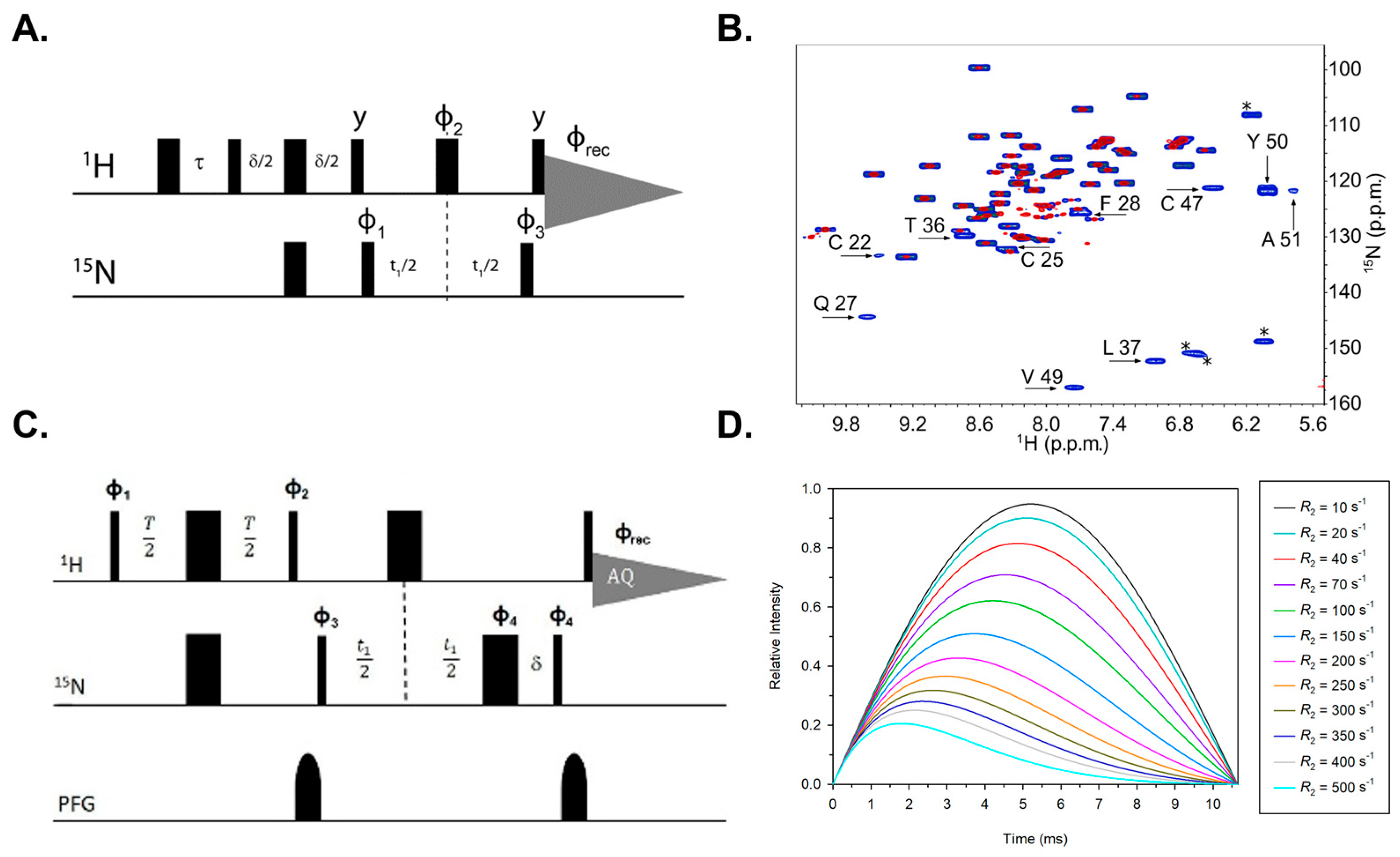
3.3. Two-Dimensional Heteronuclear ¹H-¹⁵N/¹H-¹³C Experiments

Isotope labeling techniques paved the way for the routine use of heteronuclear two-dimensional and multidimensional experiments. In biomolecular NMR, the possibility of correlating ¹H nuclei to ¹⁵N and ¹³C nuclei opened the way to deep atomic-level characterization of the structure and dynamics of macromolecules [49]. However, when systems characterized by fast nuclear relaxation are under investigation, heteronuclear 2D NMR spectroscopy starts to meet some obstacles, most of the time resulting in loss of information. This is the case of high molecular weight macromolecules (MM > 100 KDa) or systems containing paramagnetic centers. Experimental approaches aimed at circumventing the loss of information and at studying large-sized proteins and macromolecular complexes have conceptual similarities to the approaches used to study paramagnetic systems, as in both cases, the main aim is to reduce delays; however, these are outside of the scope of this review. Heteronuclear 2D NMR spectroscopy has seen remarkable advancements throughout its history, with one of the major breakthroughs being the development of the Insensitive Nuclei Enhancement by Polarization Transfer (INEPT) building block [50]. The INEPT and the experiments that have been derived from it paved the way for modern biomolecular NMR. One notable example is the Heteronuclear Single Quantum Coherence (HSQC) experiment [51], which is perhaps the most widely used NMR tool for protein fingerprinting. Neglecting relaxation, the INEPT building block provides a 100% efficient coherence transfer from a sensitive nucleus, usually hydrogen, to an insensitive nucleus, yielding an antiphase single quantum coherence. In small diamagnetic systems, the effects of relaxation can be neglected because the H/X coupling, amounting to roughly 100 Hz, allows for coherence transfer within evolution periods (of the order of 5 ms), which are short compared to transverse relaxation times. However, this is not the case when dealing with smaller scalar couplings, large molecules, or paramagnetic systems [52]. The effect of ¹H R₂ relaxation on the efficiency of coherence transfer is shown in Figure 8. When neglecting relaxation effects, the magnetization transfer efficiency is modulated by the duration of the scalar coupling evolution period and, for T = 1/2J_HX, maximizes the magnetization transfer from the sensitive ¹H nucleus to the insensitive ones. Being the proton the most sensitive probe for biomolecular NMR (highest gyromagnetic ratio within the NMR active nuclei) also implies a strong susceptibility to additional fluctuating magnetic fields, such as the ones due to unpaired electrons in the spin system, which enhance nuclear spin relaxation rates. Therefore, when the R₂ relaxation rate of the in-plane ¹H coherence increases, the magnetization transfer efficiency decays exponentially with the increase of the transverse relaxation rate. The build-up of the INEPT competes with the relaxation of the 2H_xX_z single quantum coherence, which is dominated by the ¹H_x R₂ value. Therefore, only a fraction of the initial magnetization is transferred to the heteronuclear spin, as it comes from transfer functions shown in Figure 8B. When the efficiency of the polarization transfer decreases, the maximum of the transfer function occurs for INEPT delays that are smaller than 1/2J_HX. Relaxation times below 0.1 ms (R₂ > 1000 s⁻¹) reduce the maximum of the transfer function efficiency below 10%, as shown in Figure 8C: under these conditions, direct excitation of the insensitive nucleus should provide better results than INEPT.

Tuning the INEPT delay according to the relaxation properties of the spin system is one of the major aspects, but it does not come alone: further improvements in acquisition parameters and/or pulse sequence modification are possible. Like the ¹H-¹H experiments, the acquisition time of the direct and indirect dimensions have to be adjusted according to the expected transverse relaxation rates, which, of course, are not known a priori. Generally, the frequency labeling of the heteronuclear spin in the indirect dimension does not need very high resolution and can be recorded using relatively short acquisition times without losing a large amount of magnetization. More critical is the choice of acquisition time t₂ that needs to be shortened in order to increase the S/N of fast relaxing signals, and it is ideally adjusted according to the T₂ values of the weakest observable signals.

3.3.1. Fast Relaxing Signals Require Faster Experiments

In an NMR experiment, it is crucial to reach thermal equilibrium before applying a radio frequency (RF) excitation pulse. This state of thermal equilibrium implies that the nuclear spins have achieved the Boltzmann distribution of energy levels at the specific temperature. The attainment of the state of thermal equilibrium between two transients is mandatory for the obtainment of accurate and quantitative NMR spectra. The time interval that separates two scans is called recycle delay, also known as the duty-cycle. The value of the duty-cycle for standard ¹⁵N- and ¹³C-HSQC experiments ranges from 1 s to several seconds, depending on the longitudinal relaxation time (T₁) of the excited ¹H spins. When the excited spins efficiently exchange energy with the lattice, shorter T₁ values are achieved. In the presence of a paramagnet, the dipolar interaction between electrons and nuclei acts as a very efficient relaxation source for the excited spins, thus enhancing the longitudinal relaxation rate (R₁) of the ¹H spins. As a consequence, the duty-cycle of the NMR experiment can be shortened. Typically, in paramagnetism-tailored ¹⁵N/¹³C HSQC experiments, the duty-cycle can be lowered to 1/10 of the routine recycle delay, shortening the duration of a single scan acquisition accordingly. The short duty-cycle can be compensated with an increased number of transients per experimental run, resulting in a significant increase in the signal-to-noise ratio of the experiment. Additionally, the fast cycling of the pulse sequence has the advantage that diamagnetic signals, together with spurious, unwanted resonances, i.e., the water magnetization, are partially saturated, strengthening the capability of a tailored HSQC to modulate signal intensities according to their relaxation properties.

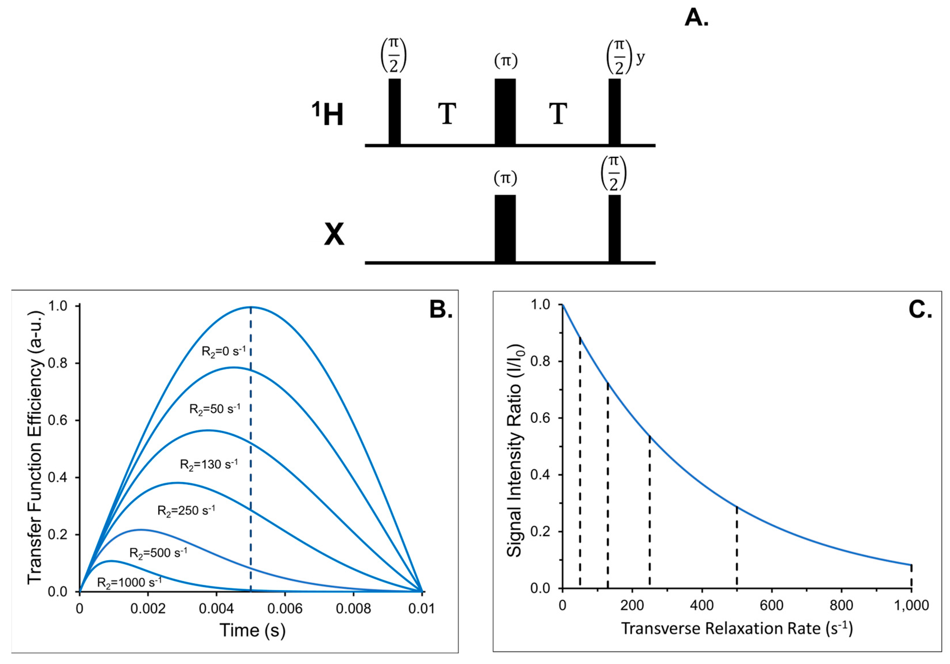
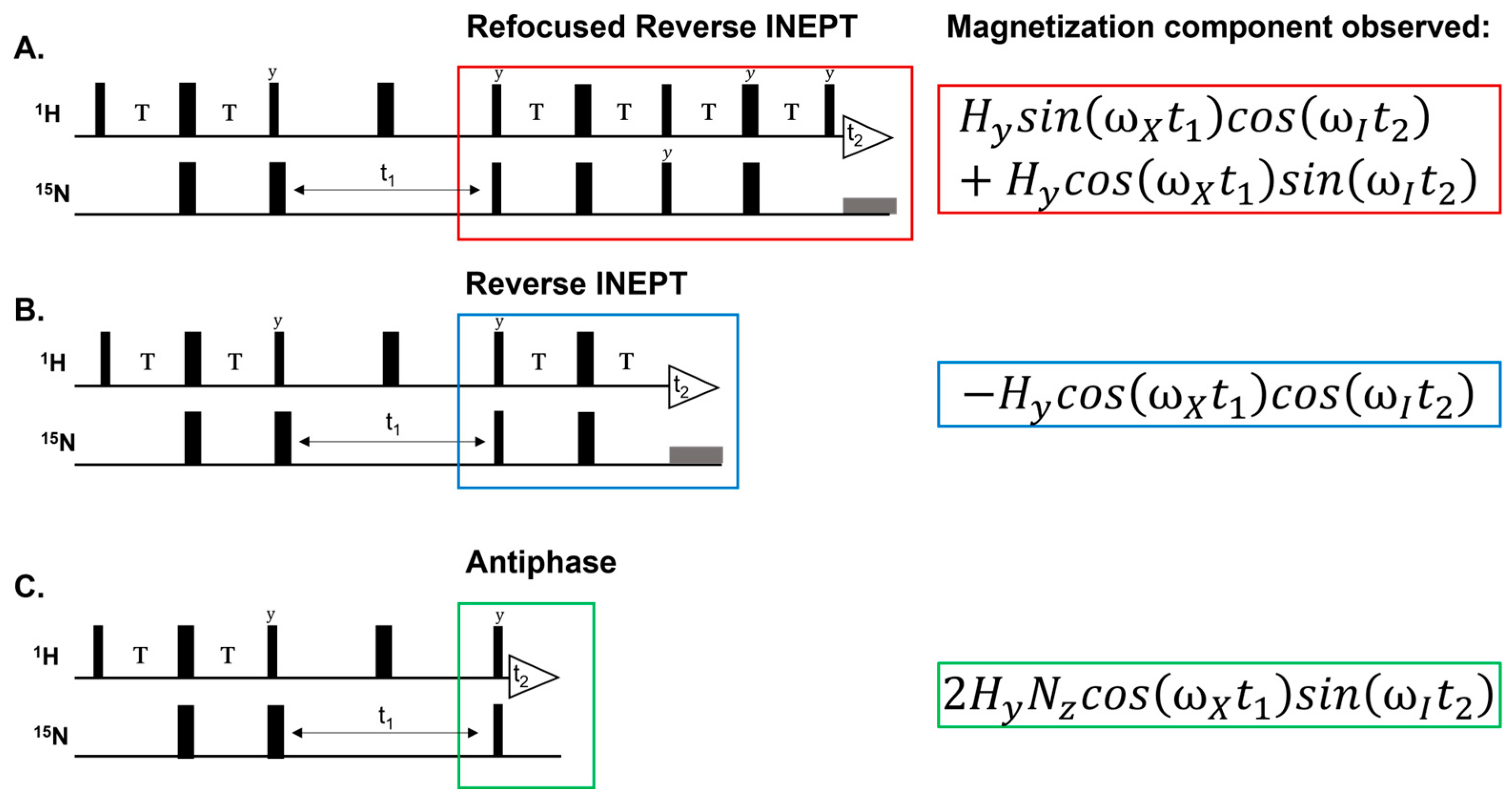
3.3.2. Antiphase Detection: Saving Time to Preserve Signals

In modern heteronuclear NMR experiments, after the ¹³C (and or ¹⁵N) spin chemical shift evolution, the magnetization is transferred back to the ¹H spin and then acquired. This is commonly accomplished with the reverse INEPT building block, with a duration equal to the initial INEPT, shown in Figure 9A. The refocusing of the -H_y component from the 2H_xX_z antiphase magnetization, followed by heteronuclear decoupling during the acquisition, gives rise to an in-phase singlet HN peak. The overall sensitivity of the experiment can be enhanced with the implementation of an additional spin echo building block, following the refocusing of the -H_y operator (Figure 9B). The sensitivity improvement scheme consists of a reverse refocused INEPT, which converts the 2H_xN_x double quantum coherence, which is unobservable with the reverse INEPT, into an additional and observable H_y single quantum coherence. As it appears immediately from the comparison of the two building blocks, the reverse refocused INEPT is a factor two longer than the reverse INEPT, resulting in severe magnetization loss for signals with large R₂ values. Indeed, the sensitivity improvement schemes are only used when working with systems characterized by T₂ relaxation rates longer than 4T (Figure 9). In paramagnetic systems, we are interested in modifying the HSQC experiment in order to make the back transfer from ¹⁵N to ¹H spin as short as possible. This can be accomplished by starting the acquisition immediately after the two 90° pulses. The antiphase (AP) detected version of the ¹⁵N-HSQC experiment, called ¹⁵N-HSQC-AP, demonstrated that signals that are broadened beyond detection in standard experiments can be recovered in the AP version experiment. The ¹⁵N-HSQC-AP experiment acquires in t₂ the antiphase component 2H_xN_z of the magnetization, generated by a 90°_x radiofrequency pulse of the ¹⁵N spin after the chemical shift evolution and followed by the 90°_y reading pulse, as shown in Figure 9C. In the absence of heteronuclear decoupling, 2H_xN_z evolves into an observable antiphase doublet. To minimize the cancellation of antiphase components, the spectra are processed with a 90° phase shift, and signals are analyzed as pseudo-singlets [53]. An additional advantage of this pulse sequence is that the removal of heteronuclear decoupling prevents the heating of the receiving coil, allowing for a faster recycling of the experiments. Combined, the short experimental duration and short duty-cycle permit an increase in the number of transients per experiment, with an overall improvement in the sensitivity for the paramagnetic signals and saturating conditions for the diamagnetic ones [54].

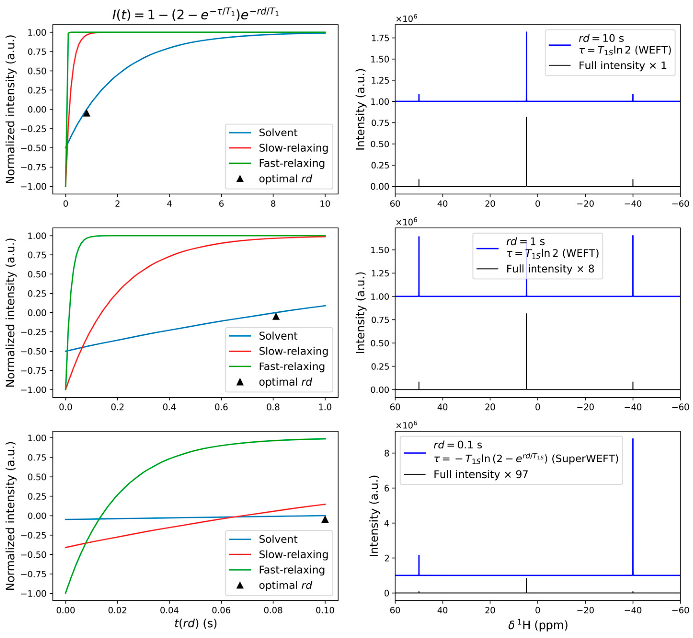
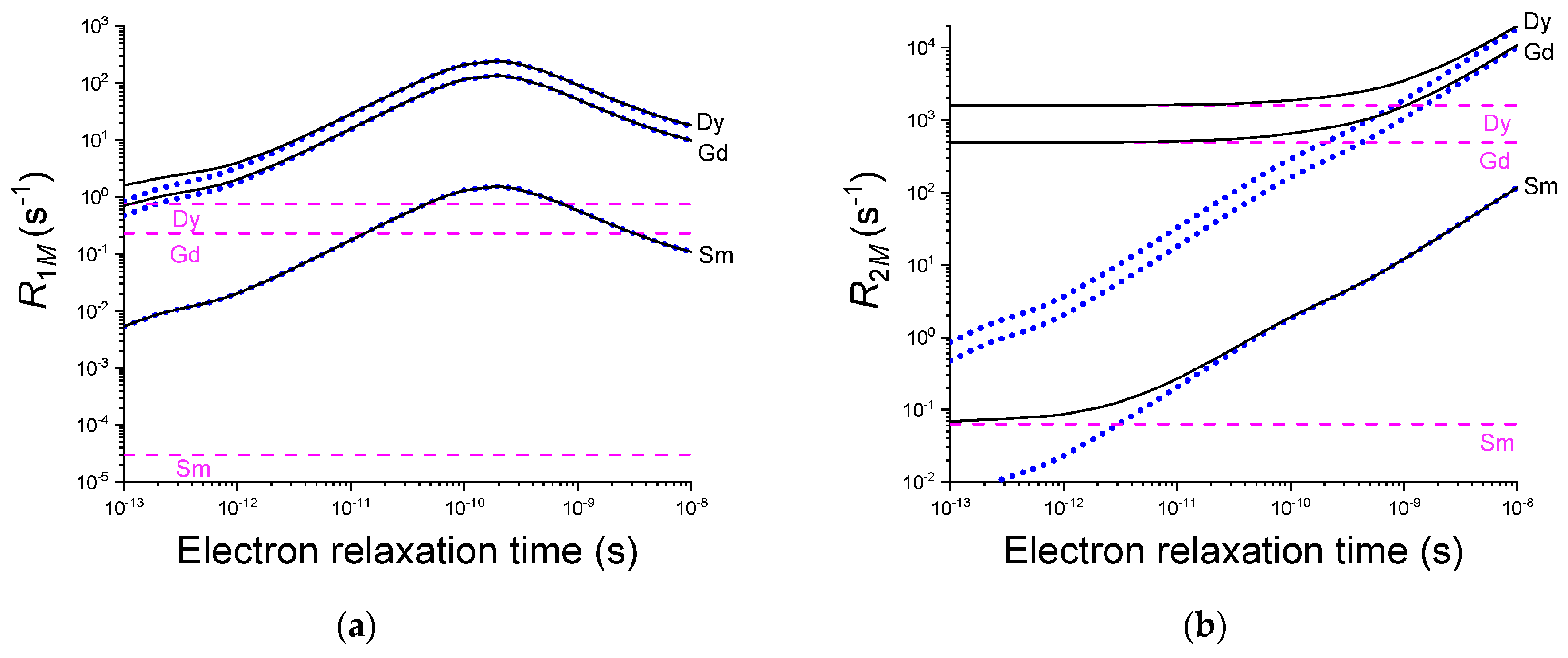
3.4. Relaxation Rate Measurements

In metalloproteins, when paramagnetism strongly impairs the possibility of obtaining an extended resonance assignment, and only a small percentage of the protein backbone can be assigned without the use of paramagnetic-tailored experiments, R₁ and R₂ relaxation rates can be used as a tool to perform signals assignment [55]. Indeed, dipolar and Curie spin terms of paramagnetic relaxation have an r⁻⁶ dependence, which is r—the distance between the metal ion and the nuclear spins. There are several factors, both experimental and theoretical, providing “caveat” of this analysis: the accuracy of measurements, the factorization of the diamagnetic contribution, uncertainty in the structural model, local mobility, the presence of the distance independent contact contribution, the fact that the r⁻⁶ relationships are based on the approximation that unpaired spin density is fully localized on the metal ion. Nevertheless, it is possible to identify potential assignments on the grounds of relaxation rates. On the other hand, the exploitation of this relationship the other way around was established more than two decades ago [56]: once the assignment is known, paramagnetic relaxation enhancement (known by the acronym PRE) can be converted into metal-to-nucleus distances and used as distance restraints in structure calculations [57,58,59].

Several experiments have been designed to measure ¹H R₁ and R₂ in paramagnetic systems. The general approach for R₁ measurements is to edit an “existing” 2D experiment (e.g., NOESY or HSQC) with the previously described inversion-recovery building block [60] (Figure 10A,B). Depending on the choice of recycle and inter-pulse delay, the 180°-τ-90° block can be used to suppress solvent and slow relaxing signals with an “ad hoc” choice of the τ delay [52] (WEFT or superWEFT filter), as already described here in the section dealing with one-dimensional experiments. When a long recycle delay allows the complete magnetization recovery to equilibrium conditions, the experiment is used to measure longitudinal relaxation rates by running a series of experiments at variable τ values [61]. Both ¹⁵N and ¹³C HSQC are able to provide accurate measurements for R₁ rates of backbone and side chain ¹H spins (Figure 10A) [62]. In the case of R₂, the usual editing scheme is a spin-echo filter inserted during or after an INEPT building block [63]. Unfortunately, the combination of spin-echo and INEPT periods prevents the identification of fast relaxing signals and, typically, allows accurate measurements of R₂ < 50 s⁻¹. To extend the measurements to a range of faster rates, the transverse relaxation delay can be directly embedded into an INEPT block (Figure 10C,D) in order to measure R₂ values up to 400 s⁻¹ [64,65].

3.5. ¹³C Direct Detected Experiments

Essentially, the approaches described throughout this article aim at minimizing the loss of the NMR information around a paramagnetic center. The region of the molecule where signals are broadened is commonly defined as an NMR-blind sphere around the metal center, and it depends on the electron correlation time of the paramagnetic metal ion. Therefore, the electronic structure of the metal ion(s) defines the threshold of signal detectability, and, of course, this cannot be circumvented. In order to decrease this detection limit, many efforts in recent years have been focused on the use of ¹³C-detected NMR experiments [66,67,68]. The rationale for the use of ¹³C direct detection is based on the fact that there is a direct relationship between PREs and the square of the gyromagnetic ratio of the studied nucleus, as shown in Figure 11. Therefore, paramagnetic relaxation effects, causing the broadening of signals beyond detection, are 16 times lower on ¹³C spins than on ¹H spins. The successful use of ¹³C direct detection instead of ¹H detection paved the way for novel strategies to assign and characterize paramagnetic systems. In particular, the CACO experiment, which correlates the intra-residue C^α and C’ spins, has very interesting features. The optimization of CACO for paramagnetic systems, shown in Figure 12, can be taken as a paradigm to extend the approach to other ¹³C-detected experiments. The experiment involves only the excitation of ¹³C spin without carrying ¹H magnetization into play, and it uses constant time evolution in the indirect dimension, which can be efficiently shortened. The In-Phase Anti-Phase (IPAP) scheme for virtual homodecoupling of C^α_zC′_y doublets can be removed, and the signal detected as antiphase, avoiding loss of information due to fast relaxation during the IPAP step. Moreover, the CACO experiment can also be used to analyze the advantages and drawbacks of the proton-start version of the experiment, which exploits ¹H as the starting polarization source [69,70].

A straightforward modification of the experiment can be obtained by inverting the C^α and C’ channels in order to perform a COCA. Recently, the application of CACO-AP and COCA-AP experiments under saturating conditions (short recycle delay) has shown that structural information regarding the topology of cluster binding ligands can be unveiled when comparing experiments with very different values for t₁ and t₂ acquisition due to the different contributions to nuclear relaxation introduced by the paramagnet. For each C^α-C’ group, the relative intensity of the two signals is correlated with the orientation of the C^α-C’ magnetization vector towards the metal center. ¹³C spins can be used as a source of structural information in solution for paramagnetic systems. Pseudocontact and contact contribution to chemical shift influence carbon nuclei in the same way they are acting on proton probes. Indeed, since the contact relaxation is less intense on carbon spins than on the proton spins, directly bound residues, which experience the Fermi interaction, become detectable. As already outlined in Figure 11, the range of distances monitored by ¹³C PREs is strongly synergistic with that of ¹H PREs and, together, strongly reinforces the battery of paramagnetism-based structural restraints [57,71]. The ¹³C^α and ¹³C′ R₁ PREs, measured by the IR-CACO-AP and IR-COCA-AP pulse sequences, were able to efficiently frame the protein structure around the metal center and to restrain the conformational space sampled by the simulated annealing process for structure calculations. An extensive combination of classical and paramagnetic-based structural restraints succeeded in obtaining NMR structures with high accuracy throughout all regions of the protein, overcoming the “limitations” that have been associated with the solution structure of paramagnetic molecules by NMR for decades.

3.6. Multidimensional Triple-Resonance Experiments

Triple resonance experiments are a combination of building blocks and acquisition parameters that, essentially, have already been discussed in the previous paragraphs. However, multidimensionality has some “caveat” that might be addressed. In 2D NMR experiments of paramagnetic systems, broad signals often overlap, resulting in crowded spectra that are challenging to interpret and sometimes even impossible. Congested and poorly resolved spectra become more informative when an additional dimension is called into the scene. The inclusion of an extra dimension (t₃) enhances signal dispersion, resulting in higher-quality spectra that enable the identification of sequential connectivity. This is particularly useful for residues that lack contact or pseudocontact shifts and are only influenced by paramagnetic relaxation enhancement. The broadening of the signals due to paramagnetism and their overlap with the diamagnetic resonances prevents an unambiguous sequence-specific assignment. An additional dimension within an NMR pulse sequence requires additional delays: taken together, the INEPT steps between heteronuclei and chemical shift evolutions can be long enough to lose a considerable part of the magnetization due to relaxation. Nonetheless, efforts have been pursued to extend the suitability of 3D NMR experiments for paramagnetic proteins. The 3D HNCA experiment correlates the chemical shift of the amide proton with the chemical shift of the covalently-bound nitrogen and alpha carbons of the same and preceding residues. This routine NMR experiment can be modified to detect paramagnetic resonances according to the parameters that we already discussed in the previous sections: i. reducing the initial H^N-to-N INEPT delay during which ¹H R₂ relaxation is active; ii. reducing the time needed for ¹H refocusing after the 2H_zN_y antiphase is generated; iii. shortening the back-transfer of the magnetization after C^α chemical shift evolution. Concerning watergate, the 3-9-19 binomial pulse is preferable to the longer soft-hard-soft 90°-y-180°-y-90° since the two soft 90° pulses are time-consuming (ca. 1 ms). It has also been shown that pulse field gradient (PFG) duration can be shortened from 1 ms to 200 us while maintaining a clean spectrum; concurrently, the time needed for the dissipation of residual circulating currents can be shortened from 200 us to 40 us. Finally, since ¹⁵N heteronuclear decoupling is active during the acquisition, a shorter recycle delay can be implemented up to 0.5 s without the risk of heating and damaging the probe-head [72]. Other multidimensional NMR experiments amenable for optimization are the 3D CBCA(CO)NH and CBCANH. These two pulse sequences are among the most popular experiments for sequential backbone assignment in proteins solution NMR [73,74,75]. The standard versions of both experiments make use of several INEPT transfer delays, crush gradients, flip-back pulses, sensitivity enhancement schemes, and echo anti-echo gradient selection. During these building blocks, relaxation is, of course, operative, and, therefore, the two experiments are expected to be unsuitable for paramagnetic optimization unless they are modified. The use of a relaxation-weighted INEPT transfer delay and the elimination of the sensitivity improvement scheme gives higher S/N. Removing the echo anti-echo gradient selection eliminates two PFGs immediately before t₃ acquisition and saves time in the most critical part of the sequence. Owing to the fact that ¹H R₂ relaxation is active during the last refocusing step of the INEPT, the removal of the two PFGs reduces the loss of magnetization due to relaxation, meanwhile enhancing the S/N ratio. The withdrawal of the gradient selection has the drawback that there is no efficient water suppression scheme left in the sequence. Anyway, this can be encompassed with a watergate scheme short enough to be compatible with the short delays of the reverse INEPT. Of course, all considerations discussed for the optimization of 2D NMR experiments concerning acquisition and processing parameters hold for 3D experiments, following the general paradigm that acquisition and recycle delays need to be shortened while the number of transients must increase in order to enhance the sensitivity of the experiment. For completeness’ sake, we remind the reader that tailored strategies to assign side chains, in the case of paramagnetic proteins, have been attempted. The coordination of paramagnetic prosthetic groups is committed to residue side chains. As a consequence, H^β, C^β, H^γ and C^γ nuclei of coordinating residues are positioned in the deepest region of the blind sphere, and hence their detection is difficult, if not impossible. Nevertheless, the use of a tailored HCCH-TOCSY was successful in recovering signals from coordinating side chains up to a distance of 4 Å from the metal ion.

4. Why

The quest for fast, relaxing, fast-shifted signals in one-dimensional experiments still represents, nowadays, a simple and valuable approach to understanding the structure and electronic properties of metal complexes and metal sites in proteins. In current inorganic chemistry literature, paramagnetic NMR (pNMR) is indeed enjoying a second youth, and most often so through very simple (or apparently simple) 1D experiments, both in solution and in the solid state. We do not aim to provide an exhaustive literature review, and we refer the interested reader to [21,29] for further reference on recent applications. To emphasize the impact and versatility of pNMR, some striking recent examples using only 1D experiments are highlighted here. The detection of a Fe-bound hydride ion shifted as much as −4000 ppm [76] represents the first case of a hydride bound to a paramagnetic metal for which the shift was predicted by DFT-based modeling and eventually observed. In the same complex, −10,000 ppm shifts were observed for the P donors. This highlights the challenge in targeting the appropriate chemical shift range when aiming to detect such nuclei and opens the per-mil ballpark for shifts [77]. Solid-state pNMR has been used in material science to address the doping homogeneity of luminescent materials, which can affect the energy transfer between sensitizer and activator ions in doped phosphors [78]. Along the way, the search and design of molecules with large magnetic susceptibility anisotropy. The observation of the patterning of the pseudocontact shift at the distance of 20 Å from the metal paved the way for the use of Co²⁺ for paramagnetic tags as an alternative to lanthanides [79].

It is also important to mention the increasingly relevant role of quantum chemical methods in relating the structural properties to the pNMR observables. The possibility of calculating the electronic structure of paramagnetic centers from first principles is offered, on the one hand, by the continuous increase in the computational power and, on the other hand, by the relentless efforts of the QC community, and the ORCA team in particular, to make QC tools understandable and useable by non-specialists [80].

As far as pNMR is concerned, Soncini and Van den Heuvel have provided the first modern QC treatment of the paramagnetic NMR shifts [81], which requires a complete treatment to reintroduce the correct field and space dependence [82].

Biological Inorganic chemistry has probably been the field where paramagnetic NMR has found many rewarding applications. Structure, coordination and electronic properties of single and multiheme proteins have been extensively characterized and reviewed [83,84,85,86,87]. Paramagnetic NMR has played a paramount role in the understanding of the electronic structure of [2Fe-2S], [3Fe-4S] and [4Fe-4S] clusters in proteins [88,89,90,91]. For all the above cases, the distribution of unpaired electron density onto the ligands allowed us to identify the type of cluster [92] and the individual oxidation states of each iron ion, quantify the antiferromagnetic couplings operative in the cluster, and assess the contribution of delocalized valence, i.e., the double-exchange term of the spin-Hamiltonian [93,94,95]. For all the small ferredoxins and HiPIPs studied, NMR offered room-temperature information that was able to complement low-temperature information taken from EPR and Mossbauer [96,97,98,99,100,101,102,103,104,105,106,107,108,109]. The methodological and instrumental advances of the last two decades have extended this approach to larger and less stable proteins, such as those involved in iron–sulfur cluster biogenesis or copper homeostasis, as well as to the mapping of protein-protein interactions responsible for cluster transfer and cluster assembly [110,111,112,113,114,115,116]. Paramagnetically shifted NMR signals have been assigned to ligands of different kinds of mono- and multi-nuclear copper clusters, allowing spectroscopically the identification of the ligands and their binding mode and the investigation of the reaction mechanisms of copper enzymes [115,117,118,119]. Paramagnetic relaxation-based NMR restraints have been successfully employed for the structure refinement of copper-containing systems [120,121,122]. Cu²⁺ has also been used as a relaxation filter that allows the selective NMR signal suppression of components in mixtures according to their complexation ability to a paramagnetic ion [123].

Like the multi-iron centers of FeS clusters, multicopper centers also display relatively sharp NMR lines due to shorter electron relaxation times as a consequence of the magnetic coupling. Again, this has allowed the use of paramagnetic NMR to explore the electronic structure and its physiological consequences [124]. The CuA center of multicopper oxidases, which has two spin-coupled copper ions in a formal Cu^1.5+ oxidation state with a thermally accessible excited state at room temperature, has been studied quite extensively. Because the observed hyperfine shift is essentially given by contact contributions, a linkage between the electronic and molecular structure of the cluster was proposed, and the Karplus-like equation governing the dependence of hyperfine shift from the H^β-C^β-S^γ-Cu dihedral angle was used to discuss the electronic excited states involved in the electron transfer mechanisms [125,126,127,128].

Ni-containing proteins have also been studied by paramagnetic NMR. In this case, the coordination number and ligand field of the d8 ion determines whether the metal ion has a ground state S = 0 or it is a high spin, S = 1. In the latter case, Ni²⁺ proteins present significant contributions from both contact and pseudocontact terms, thus puzzling the factorization of the different contributions to both shifts and relaxation. A combination of NOE experiments and the use of selectively deuterated mutants allowed the assignment of the hyperfine shifted signals of the Nickel chaperone protein Helicobacter pylori HypA as well as the characterization of its interaction with UreE, an important step of the maturation pathway of the nickel-dependent enzyme Urease [129,130]. The Ni(II)-binding properties of the intrinsically disordered protein NDRG1 have also been assessed via ¹H paramagnetic NMR.

Non-native metal substitution with paramagnetic systems [131,132], as well as the use of paramagnetic tags attached to the protein post-expression [124,133,134,135,136], has also allowed for the characterization of structure and dynamics in several biomolecular systems. The reader is referred to [6,8,9,134,137,138,139,140].

In conclusion, we can say that, thanks to many instrumental and methodological developments, paramagnetic NMR spectroscopy has been capable of surfing the wave of contemporary Inorganic Chemistry for a very long time, still contributing nowadays to diverse topics such as coordination chemistry, biological inorganic chemistry and material science. Moreover, its application also illuminates areas such as structural biology, medicinal chemistry, magnetochemistry and others. NMR of paramagnetic molecules has been capable of rejuvenating itself by expanding its capacity and exploring new applications. We hope that this review will act as a toolkit to assist newcomers in the field and to provide them with some useful basic operating instructions.

References

1. La Mar, G.N.; Horrocks, W.D., Jr.; Allen, L.C. Isotropic Proton Resonance Shifts of Some Bis-(triarylphosphine) Complexes of Cobalt(II) and Nickel(II) Dihalides. J. Chem. Phys. 1964, 41, 2126–2134. [Google Scholar] [CrossRef]
2. Thwaites, J.D.; Bertini, I.; Sacconi, L. Proton resonance studies of the solution equilibria of nickel(II) complexes with Schiff bases formed from salicylaldehydes and N,N-substituted ethylenediamines. II. Inorg. Chem. 1966, 5, 1036–1041. [Google Scholar] [CrossRef]
3. Holm, R.H.; Everett, G.W.; Horrocks, W.D., Jr. Isotropic Nuclear Magnetic Resonance Shifts in Tetrahedral Bispyridine and Bispicoline Complexes of Nickel(II). J. Am. Chem. Soc. 1966, 88, 1071. [Google Scholar] [CrossRef]
4. Kowalsky, A.J. Nuclear Magnetic Resonance Studies of Protein. J. Biol. Chem. 1962, 237, 1807–1819. [Google Scholar] [CrossRef] [PubMed]
5. La Mar, G.N.; Sacconi, L. The influence of halogen, substituent and solvent on spin delocalization in high-spin, five-coordinated 2,6-diacetylpyridinebis(N-alkylimine) nickel dihalides. J. Am. Chem. Soc. 1968, 90, 7216–7223. [Google Scholar] [CrossRef]
6. Parigi, G.; Ravera, E.; Piccioli, M.; Luchinat, C. Paramagnetic NMR restraints for the characterization of protein structural rearrangements. Curr. Opin. Struct. Biol. 2023, 80, 102595. [Google Scholar] [CrossRef]
7. Bertini, I.; Luchinat, C. NMR of Paramagnetic Molecules in Biological Systems; Benjamin/Cummings: Menlo Park, CA, USA, 1986. [Google Scholar]
8. Bertini, I.; Luchinat, C.; Parigi, G.; Ravera, E. NMR of Paramagnetic Molecules: Applications to Metallobiomolecules and Models; Elsevier: Amsterdam, The Netherlands, 2016; Volume 2. [Google Scholar]
9. Ravera, E.; Gigli, L.; Fiorucci, L.; Luchinat, C.; Parigi, G. The evolution of paramagnetic NMR as a tool in structural biology. Phys. Chem. Chem. Phys. 2022, 24, 17397–17416. [Google Scholar] [CrossRef]
10. Patt, S.L.; Sykes, B.D. Water eliminated Fourier transform NMR spectroscopy. J. Chem. Phys. 1972, 56, 3182. [Google Scholar] [CrossRef]
11. Inubushi, T.; Becker, E.D. Efficient detection of paramagnetically shifted NMR resonances by optimizing the WEFT pulse sequence. J. Magn. Reson. 1983, 51, 128–133. [Google Scholar] [CrossRef]
12. Hochmann, J.; Kellerhals, H. Proton NMR on deoxyhemoglobin: Use of a modified DEFT technique. J. Magn. Reson. 1980, 38, 23–39. [Google Scholar] [CrossRef]
13. Bondon, A.; Mouro, C. PASE (PAramagetic Signal Enhancement): A New Method for NMR Study of Paramagnetic Proteins. J. Magn. Reson. 1998, 134, 154–157. [Google Scholar] [CrossRef]
14. Helms, G.; Satterlee, J.D. Keeping PASE with WEFT: SHWEFT-PASE pulse sequences for H-1 NMR spectra of highly paramagnetic molecules. Magn. Reson. Chem. 2013, 51, 222–229. [Google Scholar] [CrossRef]
15. Levitt, M.H.; Freeman, R.; Frenkiel, T. Broadband heteronuclear decoupling. J. Magn. Reson. 1982, 47, 328–330. [Google Scholar] [CrossRef]
16. Solomon, I. Relaxation processes in a system of two spins. Phys. Rev. 1955, 99, 559–565. [Google Scholar] [CrossRef]
17. Bloembergen, N. Comments on “Proton relaxation times in paramagnetic solutions”. J. Chem. Phys. 1957, 27, 575–596. [Google Scholar] [CrossRef]
18. Gueron, M. Nuclear relaxation in macromolecules by paramagnetic ions: A novel mechanism. J. Magn. Reson. 1975, 19, 58–66. [Google Scholar] [CrossRef]
19. Vega, A.J.; Fiat, D. Nuclear Relaxation Processes of Paramagnetic Complexes. Slow. Motion Case. Mol. Phys. 1976, 31, 347–355. [Google Scholar]
20. Geraldes, C.F.G.C.; Luchinat, C. Lanthanides as shift and relaxation agents in elucidating the structure of proteins and nucleic acids. In The Lanthanides and Their Interrelations with Biosystems; CRC Press: Boca Raton, FL, USA, 2003; Volume 40, pp. 513–588. [Google Scholar]
21. Gigli, L.; Di Grande, S.; Ravera, E.; Parigi, G.; Luchinat, C. NMR for Single Ion Magnets. Magnetochemistry 2021, 7, 96. [Google Scholar] [CrossRef]
22. Neuhaus, D.; Williamson, M. The Nuclear Overhauser Effect in Structural and Conformational Analysis; VCH: New York, NY, USA, 1989. [Google Scholar]
23. Lecomte, J.T.J.; Unger, S.W.; La Mar, G.N. Practical Considerations for the Measurements of the Homonuclear Overhauser Effect on Strongly Relaxed Protons in Paramagnetic Proteins. J. Magn. Reson. 1991, 94, 112–122. [Google Scholar] [CrossRef]
24. Dugad, L.B.; La Mar, G.N.; Banci, L.; Bertini, I. Identification of localized redox states in plant-type two-iron ferredoxins using the nuclear overhauser effect. Biochemistry 1990, 29, 2263–2271. [Google Scholar] [CrossRef]
25. Ramaprasad, S.; Johnson, R.D.; La Mar, G.N. 1H-NMR Nuclear Overhauser Enhancement and Paramagnetic Relaxation Determination of Peak Assignment and the Orientation of Ile-99 FG5 in Metcyanomyoglobin. J. Am. Chem. Soc. 1984, 106, 5330–5335. [Google Scholar] [CrossRef]
26. de Ropp, J.S.; Thanabal, V.; La Mar, G.N. NMR Evidence for a Horseradish Peroxidase State with a Deprotonated Proximal Histidine. J. Am. Chem. Soc. 1985, 107, 8268–8270. [Google Scholar] [CrossRef]
27. Lecomte, J.T.J.; La Mar, G.N. The homonuclear overhauser effect in H2O solution of low-spin hemeproteins. Assignment of protons in the heme cavity of sperm whale myoglobin. Eur. Biophys. J. 1986, 13, 373–381. [Google Scholar] [CrossRef] [PubMed]
28. Santos, H.; Turner, D.L.; Xavier, A.V.; LeGall, J. Two-Dimensional NMR Studies of Electron Transfer in Cytochrome c3. J. Magn. Reson. 1984, 59, 177–180. [Google Scholar] [CrossRef]
29. Ravera, E.; Gigli, L.; Czarniecki, B.; Lang, L.; Kummerle, R.; Parigi, G.; Piccioli, M.; Neese, F.; Luchinat, C. A Quantum Chemistry View on Two Archetypical Paramagnetic Pentacoordinate Nickel(II) Complexes Offers a Fresh Look on Their NMR Spectra. Inorg. Chem. 2021, 60, 2068–2075. [Google Scholar] [CrossRef]
30. Banci, L.; Luchinat, C. Selective versus non-selective T1 experiments to determine metal-nucleus distances in paramagnetic proteins. Inorg. Chim. Acta 1998, 275–276, 373–379. [Google Scholar] [CrossRef]
31. Santana, F.S.; Perfetti, M.; Briganti, M.; Sacco, F.; Poneti, G.; Ravera, E.; Soares, J.F.; Sessoli, R. A dysprosium single molecule magnet outperforming current pseudocontact shift agents. Chem. Sci. 2022, 13, 5860–5871. [Google Scholar] [CrossRef] [PubMed]
32. Gregory, R.M.; Bain, A.D. The effects of finite rectangular pulses in NMR: Phase and intensity distortions for a spin-1/2. Concepts Magn. Reson. Part A 2009, 34A, 305–314. [Google Scholar] [CrossRef]
33. Levitt, M.H. Spin Dynamics: Basics of Nuclear Magnetic Resonance; John Wiley & Sons: Hoboken, NJ, USA, 2008. [Google Scholar]
34. Ravera, E. Phase distortion-free paramagnetic NMR spectra. J. Magn. Reson. Open 2021, 8–9, 100022. [Google Scholar] [CrossRef]
35. Aue, W.P.; Bartholdi, E.; Ernst, R.R. Two-dimensional spectroscopy. Application to nuclear magnetic resonance. J. Chem. Phys. 1976, 64, 2229–2235. [Google Scholar] [CrossRef]
36. Ernst, R.R.; Bodenhausen, G.; Wokaun, A. Principles of Nuclear Magnetic Resonance in One and Two Dimensions; Oxford University Press: London, UK, 1987. [Google Scholar]
37. Wüthrich, K. NMR of Proteins and Nucleic Acids; Wiley: New York, NY, USA, 1986. [Google Scholar]
38. Keeler, J. Understanding NMR Spectroscopy; Wiley: London, UK, 2011; p. 526. [Google Scholar]
39. Macura, S.; Ernst, R.R. Elucidation of cross relaxation in liquids by two-dimensional N.M.R. spectroscopy. Mol. Phys. 1980, 41, 95. [Google Scholar] [CrossRef]
40. Bax, A.; Davis, D.G. Practical aspects of two-dimensional transverse NOE spectroscopy. J. Magn. Reson. 1985, 63, 207–213. [Google Scholar] [CrossRef]
41. Simonis, U.; Dallas, J.L.; Walker, F.A. ROESY: A technique for establishing the existence of chemical exchange in paramagnetic model hemes with short T1 and T2 relaxation times. Inorg. Chem. 1992, 31, 5349–5350. [Google Scholar] [CrossRef]
42. Borgias, B.; Thomas, P.D.; James, T.L. Complete Relaxation Matrix Analysis (CORMA). 5.0; University of California: San Francisco, CA, USA, 1989. [Google Scholar]
43. Sørensen, O.W.; Eich, G.W.; Levitt, M.H.; Bodenhausen, G.; Ernst, R.R. Product Operator Formalism for the Description of NMR Pulse Experiments. Progr. NMR Spectrosc. 1983, 16, 163–192. [Google Scholar] [CrossRef]
44. Shriver, J. Product operators and coherence transfer in multiple-pulse NMR experiments. Concepts Magn. Reson. 1992, 4, 1–34. [Google Scholar] [CrossRef]
45. Bertini, I.; Luchinat, C.; Tarchi, D. Are true scalar proton-proton connectivities ever measured in COSY spectra of paramagnetic macromolecules? Chem. Phys. Lett. 1993, 203, 445–449. [Google Scholar] [CrossRef]
46. Qin, J.; Delaglio, F.; La Mar, G.N.; Bax, A. Distinguishing the Effects of Cross Correlation and J Coupling in COSY Spectra of Paramagnetic Protein. J. Magn. Reson. Ser. B 1993, 102, 332–336. [Google Scholar] [CrossRef]
47. Werbelow, L.G. Cross-Correlation and Interference Terms. In Encyclopedia of Nuclear Magnetic Resonance; Grant, D.M., Harris, R.K., Eds.; Wiley: Chichester, UK, 1996; pp. 4072–4079. [Google Scholar]
48. Luchinat, C.; Steuernagel, S.; Turano, P. Application of 2D-NMR techniques to paramagnetic systems. Inorg. Chem. 1990, 29, 4351–4353. [Google Scholar] [CrossRef]
49. Cavanagh, J.; Fairbrother, W.J.; Palmer, A.G., III; Rance, M.; Skelton, N.J. Protein NMR Spectroscopy. Principles and Practice; Academic Press: San Diego, CA, USA, 2007. [Google Scholar]
50. Morris, G.A.; Freeman, R. Enhancement of Nuclear Magnetic Resonance Signals by Polarization Transfer. J. Am. Chem. Soc. 1979, 101, 760–762. [Google Scholar] [CrossRef]
51. Bodenhausen, G.; Ruben, D.J. Natural abundance nitrogen-15 NMR by enhanced heteronuclear spectroscopy. Chem. Phys. Lett. 1980, 69, 185–188. [Google Scholar] [CrossRef]
52. Werbelow, L.; Thevand, A. Anomalous Nuclear Spin Relaxation Effects in the Presence of Paramagnetic Substances. J. Magn. Reson. Ser. A 1993, 101, 317–319. [Google Scholar] [CrossRef]
53. Santos, H.; Turner, D.L. 13C and proton NMR studies of horse ferricytochrome c. FEBS Lett. 1986, 194, 73–77. [Google Scholar] [CrossRef] [PubMed]
54. Bermel, W.; Bertini, I.; Felli, I.C.; Pierattelli, R. Speeding up 13C direct detection Biomolecular NMR experiments. J. Am. Chem. Soc. 2009, 131, 15339–15345. [Google Scholar] [CrossRef] [PubMed]
55. Grifagni, D.; Silva, J.M.; Cantini, F.; Piccioli, M.; Banci, L. Relaxation-based NMR assignment: Spotlights on ligand binding sites in human CISD3. J. Inorg. Biochem. 2023, 239, 112089. [Google Scholar] [CrossRef] [PubMed]
56. Bertini, I.; Donaire, A.; Luchinat, C.; Rosato, A. Paramagnetic relaxation as a tool for solution structure determination: Clostridium pasterianum ferredoxin as an example. Proteins Struct. Funct. Genet. 1997, 29, 348–358. [Google Scholar] [CrossRef]
57. Clore, G.M. Practical Aspects of Paramagnetic Relaxation Enhancement in Biological Macromolecules. Methods Enzym. 2015, 564, 485–497. [Google Scholar]
58. Iwahara, J.; Clore, G.M. Detecting transient intermediates in macromolecular binding by paramagnetic NMR. Nature 2006, 440, 1227–1230. [Google Scholar] [CrossRef]
59. Tang, C.; Ghirlando, R.; Clore, G.M. Visualization of Transient Ultra-Weak Protein Self-Association in Solution Using Paramagnetic Relaxation Enhancement. J. Am. Chem. Soc. 2008, 130, 4048–4056. [Google Scholar] [CrossRef]
60. Chen, Z.G.; de Ropp, J.S.; Hernandez, G.; La Mar, G.N. 2D NMR approaches to characterizing the molecular structure and dynamic stability of the active site for cyanide-inhibited horseradish peroxidase. J. Am. Chem. Soc. 1994, 116, 8772–8783. [Google Scholar] [CrossRef]
61. Ciofi-Baffoni, S.; Gallo, A.; Muzzioli, R.; Piccioli, M. The IR-15N-HSQC-AP experiment: A new tool for NMR spectroscopy of paramagnetic molecules. J. Biomol. NMR 2014, 58, 123–128. [Google Scholar] [CrossRef]
62. Trindade, I.B.; Invernici, M.; Cantini, F.; Louro, R.O.; Piccioli, M. PRE-driven protein NMR structures: An alternative approach in highly paramagnetic systems. FEBS J. 2021, 288, 3010–3023. [Google Scholar] [CrossRef] [PubMed]
63. Donaldson, L.W.; Skrynnikov, N.R.; Choy, W.Y.; Muhandiram, D.R.; Sarkar, B.; Forman-Kay, J.D.; Kay, L.E. Structural characterization of proteins with an attached ATCUN motif by paramagnetic relaxation enhancement NMR spectroscopy. J. Am. Chem. Soc. 2001, 123, 9843–9847. [Google Scholar] [CrossRef]
64. Invernici, M.; Trindade, I.B.; Cantini, F.; Louro, R.O.; Piccioli, M. Measuring transverse relaxation in highly paramagnetic systems. J. Biomol. NMR 2020, 74, 431–442. [Google Scholar] [CrossRef] [PubMed]
65. Banci, L.; Brancaccio, D.; Ciofi-Baffoni, S.; Del Conte, R.; Gadepalli, R.; Mikolajczyk, M.; Neri, S.; Piccioli, M.; Winkelmann, J. [2Fe-2S] cluster transfer in iron-sulfur protein biogenesis. Proc. Natl. Acad. Sci. USA 2014, 111, 6203–6208. [Google Scholar] [CrossRef]
66. Felli, I.C.; Pierattelli, R. 13C Direct Detected NMR for Challenging Systems. Chem. Rev. 2022, 122, 9468–9496. [Google Scholar] [CrossRef] [PubMed]
67. Querci, L.; Trindade, I.B.; Invernici, M.; Silva, J.M.; Cantini, F.; Louro, R.O.; Piccioli, M. NMR of Paramagnetic Proteins: 13C Derived Paramagnetic Relaxation Enhancements Are an Additional Source of Structural Information in Solution. Magnetochemistry 2023, 9, 66. [Google Scholar] [CrossRef]
68. Bermel, W.; Bertini, I.; Felli, I.C.; Kümmerle, R.; Pierattelli, R. 13C direct detection experiments on the paramagnetic oxidized monomeric copper, zinc superoxide dismutase. J. Am. Chem. Soc. 2003, 125, 16423–16429. [Google Scholar] [CrossRef] [PubMed]
69. Querci, L.; Grifagni, D.; Trindade, I.B.; Silva, J.M.; Louro, R.O.; Cantini, F.; Piccioli, M. Paramagnetic NMR to study iron sulfur proteins: 13C detected experiments illuminate the vicinity of the metal center. J. Biomol. NMR 2023, 77, 247–259. [Google Scholar] [CrossRef]
70. Mateos, B.; Conrad-Billroth, C.; Schiavina, M.; Beier, A.; Kontaxis, G.; Konrat, R.; Felli, I.C.; Pierattelli, R. The Ambivalent Role of Proline Residues in an Intrinsically Disordered Protein: From Disorder Promoters to Compaction Facilitators. J. Mol. Biol. 2020, 432, 3093–3111. [Google Scholar] [CrossRef]
71. Takeuchi, K.; Gal, M.; Shimada, I.; Wagner, G. Low-g nuclei detection experiments for biomolecular NMR. In Recent Developments in Biomolecular NMR; Clore, G.M., Potts, J., Eds.; RSC Publishing: Cambridge, UK, 2012; pp. 25–52. [Google Scholar]
72. Trindade, I.B.; Invernici, M.; Cantini, F.; Louro, R.O.; Piccioli, M. Sequence-specific assignments in NMR spectra of paramagnetic systems: A non-systematic approach. Inorg. Chim. Acta 2021, 514, 119984. [Google Scholar] [CrossRef]
73. Clore, G.M.; Gronenborn, A.M. Structure of larger proteins in solutions: Three- and four- dimensional heteronuclear NMR spectroscopy. Science 1991, 252, 1390–1399. [Google Scholar] [CrossRef] [PubMed]
74. Bertini, I.; Luchinat, C.; Rosato, A. The solution structure of paramagnetic metalloproteins. Progr. Biophys. Mol. Biol. 1996, 66, 43–80. [Google Scholar] [CrossRef] [PubMed]
75. Wuthrich, K. Protein structure determination in solution by NMR spectroscopy. J. Biol. Chem. 1990, 265, 22059–22062. [Google Scholar] [CrossRef] [PubMed]
76. Ott, J.C.; Wadepohl, H.; Enders, M.; Gade, L.H. Taking Solution Proton NMR to Its Extreme: Prediction and Detection of a Hydride Resonance in an Intermediate-Spin Iron Complex. J. Am. Chem. Soc. 2018, 140, 17413–17417. [Google Scholar] [CrossRef] [PubMed]
77. Ott, J.C.; Suturina, E.A.; Kuprov, I.; Nehrkorn, J.; Schnegg, A.; Enders, M.; Gade, L.H. Observability of Paramagnetic NMR Signals at over 10 000 ppm Chemical Shifts. Angew. Chem. Int. Ed. Engl. 2021, 60, 22856–22864. [Google Scholar] [CrossRef] [PubMed]
78. Li, W.; Smet, P.F.; Martin, L.I.D.J.; Pritzel, C.; Schmedt auf der Günne, J. Doping homogeneity in co-doped materials investigated at different length scales. Phys. Chem. Chem. Phys. 2020, 22, 818–825. [Google Scholar] [CrossRef] [PubMed]
79. Novikov, V.V.; Pavlov, A.A.; Belov, A.S.; Vologzhanina, A.V.; Savitsky, A.; Voloshin, Y.Z. Transition Ion Strikes Back: Large Magnetic Susceptibility Anisotropy in Cobalt(II) Clathrochelates. J. Phys. Chem. Lett. 2014, 5, 3799–3803. [Google Scholar] [CrossRef]
80. Neese, F. Software update: The ORCA program system, version 4.0. Wires Comput. Mol. Sci. 2018, 8, e1327. [Google Scholar] [CrossRef]
81. Van den Heuvel, W.; Soncini, A. NMR chemical shift as analytical derivative of the Helmholtz free energy. J. Chem. Phys. 2013, 138, 054113. [Google Scholar] [CrossRef]
82. Lang, L.A.-O.; Ravera, E.A.-O.; Parigi, G.A.-O.; Luchinat, C.A.-O.; Neese, F.A.-O. Solution of a Puzzle: High-Level Quantum-Chemical Treatment of Pseudocontact Chemical Shifts Confirms Classic Semiempirical Theory. J. Phys. Chem. Lett. 2020, 11, 8735–8744. [Google Scholar] [CrossRef]
83. Caillet-Saguy, C.; Piccioli, M.; Turano, P.; Lukat-Rodgers, G.; Wolff, N.; Rodgers, K.; Izadi-Pruneyre, N.; Delepierre, M.; Lecroisey, A. Heme carrier HasA: Learning about the role of the iron axial ligands in the heme uptake and release processes. J. Biol. Chem. 2012, 287, 26932–26943. [Google Scholar] [CrossRef] [PubMed]
84. Neto, S.E.; Fonseca, B.M.; Maycock, C.; Louro, R.O. Analysis of the residual alignment of a paramagnetic multiheme cytochrome by NMR. Chem. Comm. 2014, 50, 4561–4563. [Google Scholar] [CrossRef]
85. Fernandes, T.M.; Morgado, L.; Salgueiro, C.A.; Turner, D.L. Determination of the magnetic properties and orientation of the heme axial ligands of PpcA from Geobacter metallireducens by paramagnetic NMR. J. Inorg. Biochem. 2019, 198, 110718. [Google Scholar] [CrossRef] [PubMed]
86. Kleingardner, J.G.; Bowman, S.E.J.; Bren, K.L. The Influence of Heme Ruffling on Spin Densities in Ferricytochromes c Probed by Heme Core 13C NMR. Inorg. Chem. 2013, 52, 12933–12946. [Google Scholar] [CrossRef] [PubMed]
87. Worrall, J.A.; Liu, A.; Crowley, P.B.; Nocek, J.M.; Hoffman, B.M.; Ubbink, M. Myoglobin and cytochrome b5: A nuclear magnetic resonance study of a highly dynamic protein complex. Biochemistry 2002, 41, 11721–11730. [Google Scholar] [CrossRef] [PubMed]
88. Banci, L.; Camponeschi, F.; Ciofi-Baffoni, S.; Piccioli, M. The NMR contribution to protein–protein networking in Fe–S protein maturation. JBIC J. Biol. Inorg. Chem. 2018, 23, 665–685. [Google Scholar] [CrossRef] [PubMed]
89. Cai, K.; Markley, J.L. NMR as a Tool to Investigate the Processes of Mitochondrial and Cytosolic Iron-Sulfur Cluster Biosynthesis. Molecules 2018, 23, 2213. [Google Scholar] [CrossRef]
90. Xia, B.; Jenk, D.; LeMaster, D.M.; Westler, W.M.; Markley, J.L. Electron-nuclear interactions in two prototypical [2Fe-2S] proteins: Selective (chiral) deuteration and analysis of 1H and 2H NMR signals from the alpha and beta hydrogens of cysteinyl residues that ligate the iron in the active sites of human ferredoxin and Anabaena 7120 vegetative ferredoxin. Arch. Biochem. Biophys. 2000, 373, 328–334. [Google Scholar]
91. Beinert, H. Iron-sulfur proteins: Ancient structures, still full of surprises. J. Biol. Inorg. Chem. 2000, 5, 2–15. [Google Scholar] [CrossRef]
92. Invernici, M.; Selvolini, G.; Silva, J.M.; Marrazza, G.; Ciofi-Baffoni, S.; Piccioli, M. Interconversion between [2Fe-2S] and [4Fe-4S] cluster glutathione complexes. Chem. Commun. 2022, 58, 3533–3536. [Google Scholar] [CrossRef]
93. Blondin, G.; Girerd, J.J. Interplay of Electron Exchange and Electron-Transfer in Metal Polynuclear Complexes in Proteins or Chemical-Models. Chem. Rev. 1990, 90, 1359–1376. [Google Scholar] [CrossRef]
94. Mouesca, J.-M.; Lamotte, B. Iron-Sulfur clusters and their electronic and magnetic properties. Coord. Chem. Rev. 1998, 178–180, 1573–1614. [Google Scholar] [CrossRef]
95. Belinskii, M.I. Hyperfine evidence of strong double exchange in multimetallic {[Fe4S4]} active center of Escherichia coli sulfite reductase. JBIC J. Biol. Inorg. Chem. 1996, 1, 186–188. [Google Scholar] [CrossRef]
96. Krishnamoorthi, R.; Markley, J.L.; Cusanovich, M.A.; Przysiecki, C.T. Hydrogen-1 nuclear magnetic resonance investigation of Clostridium pasteurianum rubredoxin: Previously unobserved signals. Biochemistry 1986, 25, 50–54. [Google Scholar] [CrossRef] [PubMed]
97. Oh, B.-H.; Markley, J.L. Multinuclear magnetic resonance studies of the 2Fe-2S* ferredoxin from Anabaena species strain PCC 7210. 3. Detection and characterization of hyperfine-shifted nitrogen-15 and hydrogen-1 resonances of the oxidized form. Biochemistry 1990, 29, 4012–4017. [Google Scholar] [CrossRef] [PubMed]
98. Wilkens, S.J.; Xia, B.; Volkman, B.F.; Weinhold, F.; Markley, J.L.; Westler, W.M. Inadequacies of the Point-Dipole Approximation forDescribing Electron-Nuclear Interactions in Paramagnetic Proteins: Hybrid Density Functional Calculations and teh Analysis of NMR Relaxation of High Spin Iron(III) Rubredoxin. J. Phys. Chem. B 1998, 102, 8300–8305. [Google Scholar] [CrossRef]
99. Machonkin, T.E.; Westler, W.M.; Markley, J.L. Strategy for the study of paramagnetic proteins with slow electronic relaxation rates by nmr spectroscopy: Application to oxidized human [2Fe-2S] ferredoxin. J. Am. Chem. Soc. 2004, 126, 5413–5426. [Google Scholar] [CrossRef]
100. Macedo, A.L.; Moura, I.; Moura, J.J.G.; LeGall, J.; Huynh, B.H. Temperature-dependent proton NMR investigation of the electronic structure of the trinuclear iron cluster of the oxidized Desulfovibrio gigas ferredoxin II. Inorg. Chem. 1993, 32, 1101–1105. [Google Scholar] [CrossRef]
101. Goodfellow, B.J.; Macedo, A.L.; Rodrigues, P.; Moura, I.; Wray, V.; Moura, J.J.G. The solution structure of a [3Fe-4S] ferredoxin: Oxidised ferredoxin II from Desulfovibrio gigas. J. Biol. Inorg. Chem. 1999, 4, 421–430. [Google Scholar] [CrossRef]
102. Teixeira, M.; Batista, R.; Campos, A.P.; Gomes, C.; Mendes, J.; Pacheco, I.; Anemuller, S.; Hagen, W.R. A seven-iron ferredoxin from the thermoacidophilic archaeon Desulfurolobus ambivalens. Eur. J. Biochem. 1995, 227, 322–327. [Google Scholar] [CrossRef]
103. Camponeschi, F.; Piccioli, M.; Banci, L. The Intriguing mitoNEET: Functional and Spectroscopic Properties of a Unique [2Fe-2S] Cluster Coordination Geometry. Molecules 2022, 27, 8218. [Google Scholar] [CrossRef] [PubMed]
104. Camponeschi, F.; Gallo, A.; Piccioli, M.; Banci, L. The long-standing relationship between Paramagnetic NMR and Iron-Sulfur proteins: The mitoNEET example. An old method for new stories or the other way around? Magn. Reson. Discuss. 2021, 2, 203–211. [Google Scholar] [CrossRef] [PubMed]
105. Trindade, I.B.; Hernandez, G.; Lebegue, E.; Barriere, F.; Cordeiro, T.; Piccioli, M.; Louro, R.O. Conjuring up a ghost: Structural and functional characterization of FhuF, a ferric siderophore reductase from E. coli. J. Biol. Inorg. Chem. 2021, 26, 313–326. [Google Scholar] [CrossRef] [PubMed]
106. Camponeschi, F.; Ciofi-Baffoni, S.; Calderone, V.; Banci, L. Molecular Basis of Rare Diseases Associated to the Maturation of Mitochondrial [4Fe-4S]-Containing Proteins. Biomolecules 2022, 12, 1009. [Google Scholar] [CrossRef]
107. Paquete, C.M.; Saraiva, I.H.; Calçada, E.; Louro, R.O. Molecular basis for directional electron transfer. J. Biol. Chem. 2010, 285, 10370–10375. [Google Scholar] [CrossRef] [PubMed]
108. Garcia-Serres, R.; Clemancey, M.; Latour, J.M.; Blondin, G. Contribution of Mossbauer spectroscopy to the investigation of Fe/S biogenesis. J. Biol. Inorg. Chem. 2018, 23, 635–644. [Google Scholar] [CrossRef] [PubMed]
109. Welegedara, A.P.; Yang, Y.; Lee, M.D.; Swarbrick, J.D.; Huber, T.; Graham, B.; Goldfarb, D.; Otting, G. Double-Arm Lanthanide Tags Deliver Narrow Gd3+-Gd3+ Distance Distributions in Double Electron-Electron Resonance (DEER) Measurements. Chem-Eur. J. 2017, 23, 11694–11702. [Google Scholar] [CrossRef]
110. Srour, B.; Gervason, S.; Hoock, M.H.; Monfort, B.; Want, K.A.-O.; Larkem, D.; Trabelsi, N.; Landrot, G.A.-O.X.; Zitolo, A.A.-O.; Fonda, E.A.-O.; et al. Iron Insertion at the Assembly Site of the ISCU Scaffold Protein Is a Conserved Process Initiating Fe-S Cluster Biosynthesis. J. Am. Chem. Soc. 2022, 144, 17496–17515. [Google Scholar] [CrossRef]
111. Camponeschi, F.; Muzzioli, R.; Ciofi-Baffoni, S.; Piccioli, M.; Banci, L. Paramagnetic 1H NMR Spectroscopy to Investigate the Catalytic Mechanism of Radical S-Adenosylmethionine Enzymes. J. Mol. Biol. 2019, 431, 4514–4522. [Google Scholar] [CrossRef]
112. Honarmand Ebrahimi, K.; Ciofi-Baffoni, S.; Hagedoorn, P.L.; Nicolet, Y.; Le Brun, N.E.; Hagen, W.R.; Armstrong, F.A. Iron-sulfur clusters as inhibitors and catalysts of viral replication. Nat. Chem. 2022, 14, 253–266. [Google Scholar] [CrossRef]
113. Brancaccio, D.; Gallo, A.; Piccioli, M.; Novellino, E.; Ciofi-Baffoni, S.; Banci, L. [4Fe-4S] Cluster Assembly in Mitochondria and Its Impairment by Copper. J. Am. Chem. Soc. 2017, 139, 719–730. [Google Scholar] [CrossRef] [PubMed]
114. Ji, Y.; Wei, L.; Da, A.; Stark, H.; Hagedoorn, P.L.; Ciofi-Baffoni, S.; Cowley, S.A.; Louro, R.O.; Todorovic, S.; Mroginski, M.A.; et al. Radical-SAM dependent nucleotide dehydratase (SAND), rectification of the names of an ancient iron-sulfur enzyme using NC-IUBMB recommendations. Front. Mol. Biosci. 2022, 9, 1032220. [Google Scholar] [CrossRef] [PubMed]
115. Bennett, S.P.; Crack, J.C.; Puglisi, R.; Pastore, A.; Le Brun, N.E. Native mass spectrometric studies of IscSU reveal a concerted, sulfur-initiated mechanism of iron-sulfur cluster assembly. Chem. Sci. 2022, 14, 78–95. [Google Scholar] [CrossRef] [PubMed]
116. Gervason, S.; Larkem, D.; Mansour, A.B.; Botzanowski, T.; Muller, C.S.; Pecqueur, L.; Le Pavec, G.; Delaunay-Moisan, A.; Brun, O.; Agramunt, J.; et al. Physiologically relevant reconstitution of iron-sulfur cluster biosynthesis uncovers persulfide-processing functions of ferredoxin-2 and frataxin. Nat. Commun. 2019, 10, 3566. [Google Scholar] [CrossRef] [PubMed]
117. Bubacco, L.; Salgado, J.; Tepper, A.W.J.W.; Vijgenboom, E.; Canters, G.W. 1H NMR spectroscopy of the binuclear Cu(II) active site of Streptomyces antibioticus tyrosinase. FEBS Lett. 1999, 442, 215–220. [Google Scholar] [CrossRef]
118. Zaballa, M.-E.; Ziegler, L.; Kosman, D.J.; Vila, A.J. NMR Study of the Exchange Coupling in the Trinuclear Cluster of the Multicopper Oxidase Fet3p. J. Am. Chem. Soc. 2010, 132, 11191–11196. [Google Scholar] [CrossRef] [PubMed]
119. Machczynski, M.C.; Babicz, J.T. Correlating the structures and activities of the resting oxidized and native intermediate states of a small laccase by paramagnetic NMR. J. Inorg. Biochem. 2016, 159, 62–69. [Google Scholar] [CrossRef]
120. Arnesano, F.; Banci, L.; Bertini, I.; Felli, I.C.; Luchinat, C.; Thompsett, A.R. A strategy for the NMR characterization of type II copper(II) proteins: The case of the copper trafficking protein CopC from Pseudomonas Syringae. J. Am. Chem. Soc. 2003, 125, 7200–7208. [Google Scholar] [CrossRef]
121. Abelein, A.; Ciofi-Baffoni, S.; Mörman, C.; Kumar, R.; Giachetti, A.; Piccioli, M.; Biverstål, H. Molecular Structure of Cu(II)-Bound Amyloid-β Monomer Implicated in Inhibition of Peptide Self-Assembly in Alzheimer’s Disease. JACS Au 2022, 2, 2571–2584. [Google Scholar] [CrossRef]
122. Scanu, S.; Foerster, J.M.; Ullmann, G.M.; Ubbink, M. Role of Hydrophobic Interactions in the Encounter Complex Formation of the Plastocyanin and Cytochrome f Complex Revealed by Paramagnetic NMR Spectroscopy. J. Am. Chem. Soc. 2013, 135, 7681–7692. [Google Scholar] [CrossRef]
123. Correa, J.; Garcia-Barandela, A.; Socias-Pinto, L.; Fernandez-Megia, E. Filtering the NMR Spectra of Mixtures by Coordination to Paramagnetic Cu2+. Anal. Chem. 2022, 94, 10907–10911. [Google Scholar] [CrossRef] [PubMed]
124. Miao, Q.; Nitsche, C.; Orton, H.; Overhand, M.; Otting, G.; Ubbink, M. Paramagnetic Chemical Probes for Studying Biological Macromolecules. Chem. Rev. 2022, 122, 9571–9642. [Google Scholar] [CrossRef] [PubMed]
125. Luchinat, C.; Soriano, A.; Djinovic-Carugo, K.; Saraste, M.; Malmström, B.G.; Bertini, I. Electronic and geometric structure of the CuA site studied by 1H NMR in a soluble domain of cytochrome c oxidase from Paracoccus denitrificans. J. Am. Chem. Soc. 1997, 119, 11023–11027. [Google Scholar] [CrossRef]
126. Salgado, J.; Warmerdam, G.; Bubacco, L.; Canters, G.W. Understanding the electronic properties of the CuA site from the soluble domain of cytochrome c oxidase through paramagnetic 1H NMR. Biochemistry 1998, 37, 7378–7389. [Google Scholar] [CrossRef] [PubMed]
127. Fernández, C.O.; Cricco, J.A.; Slutter, C.E.; Richards, J.H.; Gray, H.B.; Vila, A.J. Axial ligand modulation of the electronic structures of binuclear copper sites: Analysis of paramagnetic 1H NMR spectra of Met160Gln CuA. J. Am. Chem. Soc. 2001, 123, 11678–11685. [Google Scholar] [CrossRef]
128. Abriata, L.A.; Ledesma, G.N.; Pierattelli, R.; Vila, A.J. Electronic structure of the ground and excited states of the CuA site by NMR spectroscopy. J. Am. Chem. Soc. 2009, 131, 1939–1946. [Google Scholar] [CrossRef]
129. Spronk, C.; Zerko, S.; Gorka, M.; Kozminski, W.; Bardiaux, B.; Zambelli, B.; Musiani, F.; Piccioli, M.; Basak, P.; Blum, F.C.; et al. Structure and dynamics of Helicobacter pylori nickel-chaperone HypA: An integrated approach using NMR spectroscopy, functional assays and computational tools. J. Biol. Inorg. Chem. 2018, 23, 1309–1330. [Google Scholar] [CrossRef]
130. Zambelli, B.; Basak, P.; Hu, H.; Piccioli, M.; Musiani, F.; Broll, V.; Imbert, L.; Boisbouvier, J.; Maroney, M.J.; Ciurli, S. The structure of the high-affinity nickel-binding site in the Ni,Zn-HypA•UreE2 complex. Metallomics 2023, 15, mfad003. [Google Scholar] [CrossRef]
131. Bertini, I.; Luchinat, C. Cobalt(II) as a probe of the structure and function of carbonic anhydrase. Acc. Chem. Res. 1983, 16, 272–279. [Google Scholar] [CrossRef]
132. Cerofolini, L.; Staderini, T.; Giuntini, S.; Ravera, E.; Fragai, M.; Parigi, G.; Pierattelli, R.; Luchinat, C. Long-range paramagnetic NMR data can provide a closer look on metal coordination in metalloproteins. J. Biol. Inorg. Chem. 2018, 23, 71–80. [Google Scholar] [CrossRef]
133. Zhu, W.; Yang, D.T.; Gronenborn, A.M. Ligand-Capped Cobalt(II) Multiplies the Value of the Double-Histidine Motif for PCS NMR Studies. J. Am. Chem. Soc. 2023, 145, 4564–4569. [Google Scholar] [CrossRef] [PubMed]
134. Herath, I.D.; Breen, C.; Hewitt, S.H.; Berki, T.R.; Kassir, A.F.; Dodson, C.; Judd, M.; Jabar, S.; Cox, N.; Otting, G.; et al. A Chiral Lanthanide Tag for Stable and Rigid Attachment to Single Cysteine Residues in Proteins for NMR, EPR and Time-Resolved Luminescence Studies. Chemistry 2021, 27, 13009–13023. [Google Scholar] [CrossRef] [PubMed]
135. Nitsche, C.; Otting, G. Intrinsic and Extrinsic Paramagnetic Probes. In Paramagnetism in Experimental Biomolecular NMR; Luchinat, C., Parigi, G., Ravera, E., Eds.; Royal Society of Chemistry: Cambridge, UK, 2018; Volume 1, pp. 189–218. [Google Scholar]
136. Miao, Q.; Liu, W.M.; Kock, T.; Blok, A.; Timmer, M.; Overhand, M.; Ubbink, M. A Double-Armed, Hydrophilic Transition Metal Complex as a Paramagnetic NMR Probe. Angew. Chem. Int. Ed. Engl. 2019, 58, 13093–13100. [Google Scholar] [CrossRef] [PubMed]
137. Wu, F.J.; Rieder, P.S.; Abiko, L.A.; Rossler, P.; Gossert, A.D.; Haussinger, D.; Grzesiek, S. Nanobody GPS by PCS: An Efficient New NMR Analysis Method for G Protein Coupled Receptors and Other Large Proteins. J. Am. Chem. Soc. 2022, 144, 21728–21740. [Google Scholar] [CrossRef]
138. Muntener, T.; Joss, D.; Haussinger, D.; Hiller, S. Pseudocontact Shifts in Biomolecular NMR Spectroscopy. Chem. Rev. 2022, 122, 9422–9467. [Google Scholar] [CrossRef]
139. Parker, D.; Suturina, E.A.; Kuprov, I.; Chilton, N.F. How the Ligand Field in Lanthanide Coordination Complexes Determines Magnetic Susceptibility Anisotropy, Paramagnetic NMR Shift, and Relaxation Behavior. Acc. Chem. Res. 2020, 53, 1520–1534. [Google Scholar] [CrossRef]
140. Mori, M.; Kateb, F.; Bodenhausen, G.; Piccioli, M.; Abergel, D. Towards structural dynamics: Protein motions viewed by chemical shift modulations and direct detection of C’N multiple-quantum relaxation. J. Am. Chem. Soc. 2010, 132, 3594–3600. [Google Scholar] [CrossRef]
Figure 1. Scheme of a simple one-dimensional pulse-acquisition NMR experiment, composed of the interscan delay, a pulse, the delay between pulse and acquisition (vide infra) and the signal acquisition.
Inorganics 12 00015 g001
Figure 2. Typical values of electron relaxation time (τe), magnetic susceptibility (χ, spin-only values, equal to [μ0μB2ge2S(S+1)]/3KT and effective values, reported in parenthesis), and its axial anisotropy (Δχax) of transition metal ions. The typical radii of blind spheres (black) and spheres with 1H PREs larger than 0.1 s−1 (green) and the maximum distances of nuclei in axial position with PCSs of 0.05 ppm (blue) are also shown for a protein with the reorientation time of 10 ns at 700 MHz (HS = high spin, LS = low spin). Reproduced with permission from [9].
Inorganics 12 00015 g002
Figure 3. Simulation of 1D 1H NMR spectra for signals of different T2 (2 s−1, 5 s−1, 10 s−1) processed for different DE values (A) and at different TDEFF (B). A DW = 3 us and TD = 65 k data points were used, corresponding to effective acquisition times for the three spectra in (B) of 0.200 s, 0.0614 s, and 0.0154 s.
Inorganics 12 00015 g003
Figure 4. On the left, the normalized signal intensity curves for WEFT and SuperWEFT pulse sequences for 3 different relaxing signals: the solvent (T1 = 2 s, I = 1, 4.75 ppm), a slow-relaxing signal (T1 = 200 ms, I = 0.02, 50 ppm) and a fast-relaxing signal (T1 = 20 ms, I = 0.02, −40 ppm). The curves’ equation is reported above, and the optimal recycle delay (the time interval between two scans, also known as duty-cycle, rd) values are pointed out by the symbol ▲. On the right, the superposition of two spectra: in black, the full intensity spectra (rd = 10 s, τ = 10 s), and in blue, the reduced intensity spectra at different rd and optimal τ. rd is the delay that precedes the 180° pulse. τ is the delay between the 180° pulse and the acquisition pulse.
Inorganics 12 00015 g004
Figure 5. Solomon (dotted blue lines) and Curie (dashed pink lines) contributions to nuclear longitudinal (a) and transverse (b) paramagnetic relaxation (solid black lines) as a function of the electron relaxation time for samarium(III) (J = 5/2), gadolinium(III) (J = 7/2) and dysprosium(III) (J = 15/2). A non-exchangeable 1H nucleus was considered at a distance r = 10 Å from the paramagnetic metal in a molecule with a reorientation time τr = 10 ns in a magnetic field of 900 MHz proton Larmor frequency. Reproduced with permission from [21].
Inorganics 12 00015 g005
Figure 6. 1D difference traces obtained by irradiating the signal at 229 ppm (top) and the signal at −8.5 ppm (bottom). In the top trace, the response of the signal at 288 ppm is negative, indicating magnetization transfer through NOE. In the bottom trace, the response of the signal at −1.9 ppm is positive, indicating saturation transfer through chemical exchange. Reproduced with permission from [29].
Inorganics 12 00015 g006
Figure 7. Simulation of 1D 1H NMR spectra for signals of different T2 (2 s−1, 5 s−1, 10 s−1) with pulse-induced phase distortion (red) and DE-induced phase distortion (green). The pulse-induced phase distortion is calculated using the equations in [32].
Inorganics 12 00015 g007
Figure 8. (A) pulse sequence for INEPT. The narrow and broad black rectangles denote 90° and 180° flip angle pulses, respectively. X refers to nuclei such as 13C or 15N. Τ delay is defined as 1/4JHX. The phase of the pulses is x when not indicated. (B), efficiency of the transfer function in the absence (R2 = 0 s−1) and in the presence of relaxation (R2 = 50, 130, 250, 500 and 1000 s−1). A dotted line, positioned at 0.005 s, is included to emphasize the maximum of the polarization transfer function in the negligible relaxation scenario. (C) The panel displays the Signal Intensity Ratio weighted by escalating transverse relaxation rates. Dotted lines are placed to highlight specific SIR values corresponding to each transverse relaxation rate utilized in panel B.
Inorganics 12 00015 g008
Figure 9. The fundamental HSQC pulse sequence (A) and sensitivity improvement implementation though a refocused reverse INEPT scheme (B). The narrow and broad black rectangles denote 90° and 180° flip angle pulses, respectively. Τ represents the scalar coupling evolution time, defined as 1/4JHX. The phase of the pulses is x when not indicated. Heteronuclear decoupling in the indirect dimension is reported as wide gray rectangles. Indirect and direct acquisition times are indicated as t1 and t2, respectively. The sensitivity improvement scheme generates a couple of pure single quantum coherences (red rectangle) with respect to the classical INEPT step (blue rectangle). The removal of the reverse INEPT building block (C) generates an antiphase single quantum coherence that is directly detected without heteronuclear decoupling in the indirect dimension. In all rectangles, only the y component of the signal product operator is shown.
Inorganics 12 00015 g009
Figure 10. IR-HSQC-AP pulse sequence (A,B) 1H-15N correlation spectra and resulting spectrum acquired on a 15N-labelled sample of the High Potential Iron Protein (HiPIP) PioC protein, with a standard HSQC (red) and paramagnetic optimized IR-HSQC-AP (blue) pulse sequences. Signals marked with asterisks are folded peaks arising from side chains. [62] In this specific case, the inversion recovery building block is used as a relaxation filter to suppress the diamagnetic background. Black labels indicate 11 additional cross-peaks recovered with the paramagnetic tailored experiment. R2-weighted HSQC-AP pulse sequence (C) and relative intensity after the initial INEPT, simulated at different 1H R2 values (D) [64].
Inorganics 12 00015 g010
Figure 11. Paramagnetic dipolar contribution to R2 relaxation reported for a small protein (τr = 3.3 ns). The electron correlation time (τe) is assumed to be equal to 6.0 ps, in the absence of chemical exchange (τM = 0 s). Curves are simulated for 1H, 13C and 15N nuclei resonating at 500, 125 and 50 MHz, respectively. Limits of detectability, expressed as signal line broadening (Hz), are set from a minimum of 1 Hz to a reasonable maximum of 1000 Hz.
Inorganics 12 00015 g011
Figure 12. The CACO-AP pulse sequence scheme implemented with a Hα-to-Cα INEPT delay Τ of 2.7 ms. The phase cycle reported in the figure is as follows: φ1 = x, φ2 = y, φ3 = x,−x, φ4 = x,x,x,x,y,y,y,y, φ5 = x,x,−x,−x, φ6 = x,−x,−x,x,−x,x,x,−x. PFG used in the sequence has a sine bell shape and duration of 1 ms.
Inorganics 12 00015 g012
Disclaimer/Publisher’s Note: The statements, opinions and data contained in all publications are solely those of the individual author(s) and contributor(s) and not of MDPI and/or the editor(s). MDPI and/or the editor(s) disclaim responsibility for any injury to people or property resulting from any ideas, methods, instructions or products referred to in the content.