Dynamics of Fractional Vortex Beams at Fraunhofer Diffraction Zone


Abstract
:
1. Introduction
2. Theoretical Insights and Numerical Results
3. Experimental Results and Discussion
4. Conclusions
Author Contributions
Funding
Conflicts of Interest
Abbreviations
| FVBs | Fractional vortex beams |
| TC | Topological charge |
| SLM | Spatial light modulator |
| FWHM | Full width at half maximum |
| CMOS | Complementary Metal-oxide semiconductor |
| CCD | Charge-coupled device |
| NF | Neutral filter |
References
- Tao, S.H.; Yuan, X.-C.; Lin, J.; Peng, X.; Niu, H.B. Fractional optical vortex beam induced rotation of particles. Opt. Express 2005, 13, 7726–7731. [Google Scholar] [CrossRef]
- Tkachenko, G.; Chen, M.; Dholakia, K.; Mazilu, M. Is it possible to create a perfect fractional vortex beam? Optica 2017, 4, 330–333. [Google Scholar] [CrossRef] [Green Version]
- Alperin Samuel, N.; Siemens Mark, E. Angular Momentum of Topologically Structured Darkness. Phys. Rev. Lett. 2017, 119, 203902. [Google Scholar] [CrossRef] [Green Version]
- Gbur, G. Fractional vortex Hilbert’s Hotel. Optica 2016, 3, 222–225. [Google Scholar] [CrossRef]
- Basistiy, I.V.; Pas’ko, V.A.; Slyusar, V.V.; Soskin, M.S.; Vasnetsov, M.V. Synthesis and analysis of optical vortices with fractional topological charges. J. Opt. A Pure Appl. Opt. 2004, 6, S166–S169. [Google Scholar] [CrossRef]
- Berry, M.V. Optical vortices evolving from helicoidal integer and fractional phase steps. J. Opt. A Pure Appl. Opt. 2004, 6, 259–268. [Google Scholar] [CrossRef]
- Leach, J.; Yao, E.; Padgett, M.J. Observation of the vortex structure of a non-integer vortex beam. New J. Phys. 2004, 6, 71. [Google Scholar] [CrossRef]
- Lee, W.; Yuan, X.-C.; Dholakia, K. Experimental observation of optical vortex evolution in a Gaussian beam with an embedded fractional phase step. Opt. Commun. 2004, 239, 129–135. [Google Scholar] [CrossRef] [Green Version]
- Jesus-Silva, A.J.; Fonseca, E.J.S.; Hickmann, J.M. Study of the birth of a vortex at Fraunhofer zone. Opt. Lett. 2012, 37, 4552–4554. [Google Scholar] [CrossRef] [PubMed]
- Wen, J.; Wang, L.-G.; Yang, X.; Zhang, J.; Zhu, S.-Y. Vortex strength and beam propagation factor of fractional vortex beams. Opt. Express 2019, 27, 5893–5904. [Google Scholar] [CrossRef] [PubMed] [Green Version]
- Kotlyar, V.; Kovalev, A.; Nalimov, A.; Porfirev, A. Evolution of a vortex with an initial fractional topological charge. Phys. Rev. A 2020, 102, 023516. [Google Scholar] [CrossRef]
- Kotlyar, V.; Kovalev, A.; Volyar, A. Topological Charge of a linear combination of optical vortices: Topological competition. Opt. Express 2020, 28, 8266–8280. [Google Scholar] [CrossRef] [PubMed]
- Zhang, H.; Zeng, J.; Lu, X.; Wang, Z.; Zhao, C.; Cai, Y. Review on fractional vortex beam. Nanophotonics 2022, 11, 241–273. [Google Scholar] [CrossRef]
- Liu, Z.W.; Yan, S.; Liu, H.G.; Chen, X.F. Superhigh resolution recognition of optical vortex modes assisted by a deep-learning method. Phys. Rev. Lett. 2019, 123, 183902. [Google Scholar] [CrossRef] [PubMed]


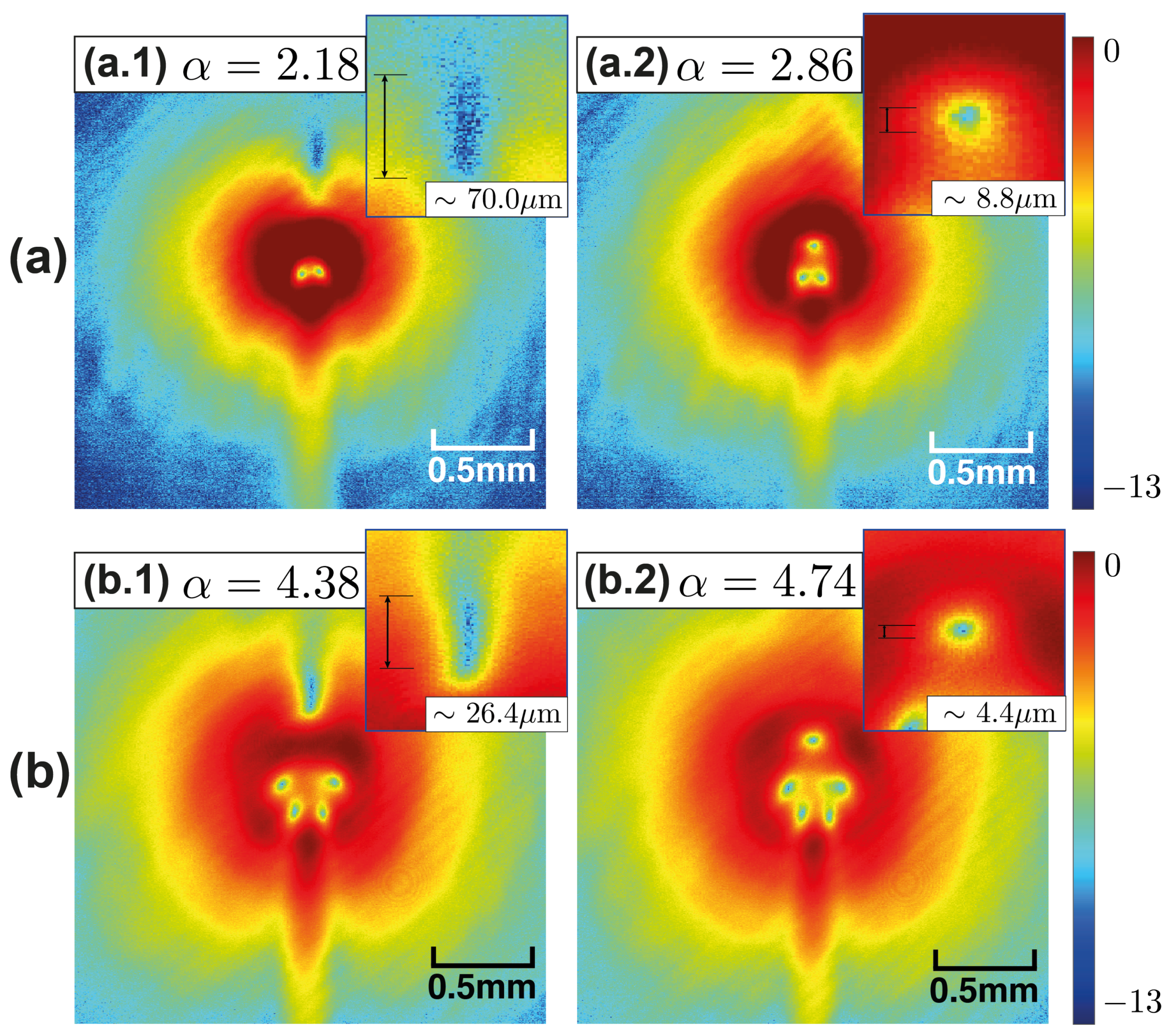
| Input | d (µm) | d (µm) | Err | |
|---|---|---|---|---|
| 2.18 | 462.3 | 462.0 ± 35.2 | 2.18 ± 0.02 | <1% |
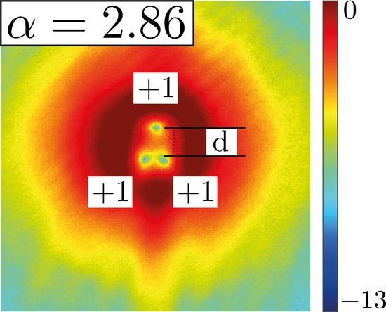
| 2.86 | 88.0 | 83.6 ± 4.4 | 2.87 ± 0.01 | <0.7% |
| 4.38 | 352.3 | 358.6 ± 13.2 | 4.40 ± 0.04 | <1% |
| 4.74 | 176.1 | 176.0 ± 2.2 | 4.74 ± 0.02 | <0.4% |
Publisher’s Note: MDPI stays neutral with regard to jurisdictional claims in published maps and institutional affiliations. |
© 2022 by the authors. Licensee MDPI, Basel, Switzerland. This article is an open access article distributed under the terms and conditions of the Creative Commons Attribution (CC BY) license (https://creativecommons.org/licenses/by/4.0/).
Share and Cite
Peters, E.; Funes, G.; Martínez-León, L.; Tajahuerce, E. Dynamics of Fractional Vortex Beams at Fraunhofer Diffraction Zone. Photonics 2022, 9, 479. https://doi.org/10.3390/photonics9070479
Peters E, Funes G, Martínez-León L, Tajahuerce E. Dynamics of Fractional Vortex Beams at Fraunhofer Diffraction Zone. Photonics. 2022; 9(7):479. https://doi.org/10.3390/photonics9070479
Chicago/Turabian StylePeters, Eduardo, Gustavo Funes, L. Martínez-León, and Enrique Tajahuerce. 2022. "Dynamics of Fractional Vortex Beams at Fraunhofer Diffraction Zone" Photonics 9, no. 7: 479. https://doi.org/10.3390/photonics9070479
APA StylePeters, E., Funes, G., Martínez-León, L., & Tajahuerce, E. (2022). Dynamics of Fractional Vortex Beams at Fraunhofer Diffraction Zone. Photonics, 9(7), 479. https://doi.org/10.3390/photonics9070479