Wavefront Fitting over Arbitrary Freeform Apertures via CSF-Guided Progressive Quasi-Conformal Mapping

Abstract

In freeform optical metrology, wavefront fitting over non-circular apertures is hindered by the loss of Zernike polynomial orthogonality and severe sampling grid distortion inherent in standard conformal mappings. To address the resulting numerical instability and fitting bias, we propose a unified framework curve-shortening flow (CSF)-guided progressive quasi-conformal mapping (CSF-QCM), which integrates geometric boundary evolution with topology-aware parameterization. CSF-QCM first smooths complex boundaries via curve-shortening flow, then solves a sparse Laplacian system for harmonic interior coordinates, thereby establishing a stable diffeomorphism between physical and canonical domains. For doubly connected apertures, it preserves topology by computing the conformal modulus via Dirichlet energy minimization and simultaneously mapping both boundaries. Benchmarked against state-of-the-art methods (e.g., Fornberg, Schwarz–Christoffel, and Ricci flow) on representative irregular apertures, CSF-QCM suppresses area distortion and restores discrete orthogonality of the Zernike basis, reducing the Gram matrix condition number from >900 to <8. This enables high-precision reconstruction with RMS residuals as low as $3\times {10}^{-3}\lambda$ and up to 92% lower fitting errors than baselines. The framework provides a unified, computationally efficient, and numerically stable solution for wavefront reconstruction in complex off-axis and freeform optical systems.

1. Introduction

Advanced optical manufacturing increasingly demands nanometer surface accuracy for freeform optical elements [1,2]. Wavefront testing is therefore a critical component of the metrology pipeline, and reconstruction accuracy directly affects the reliability of closed-loop fabrication. Conventional wavefront analysis commonly relies on Zernike polynomials defined on the unit disk, where their orthogonality and physical interpretability are fully advantageous [3,4,5].

Due to these mathematical properties, the utility of Zernike polynomials extends far beyond manufacturing. They are widely adopted in optical surface testing (interferometry) and adaptive optics (AO), where they are extensively employed to model atmospheric turbulence [6,7] and control deformable mirrors for wavefront correction. In particular, the integration of Zernike modes with Shack–Hartmann wavefront sensors (SHWS) has become a cornerstone in fields ranging from astronomical instrumentation to biological microscopy [8], enabling precise quantification of refractive aberrations.

However, these classical applications typically assume a circular pupil. For arbitrary freeform apertures (e.g., non-convex regions, high-aspect-ratio pupils, or apertures with obscurations), the mismatch between the physical support and the unit disk induces significant modal crosstalk and coefficient coupling [9,10,11].

Two broad strategies have been employed to mitigate these limitations.

First, customized orthogonal bases can be constructed via Gram–Schmidt orthogonalization or singular value decomposition (SVD) on sampled apertures [12,13]. Recent advancements have further optimized orthogonal fitting algorithms for aberration removal on arbitrary-shaped apertures [14], and data-driven approaches utilizing deep neural networks have also emerged [15]. While effective, these numerical approaches face a critical challenge: their stability is heavily dependent on the quality of node selection.

To address this, recent studies [16] have demonstrated that transplanting optimized sampling patterns (e.g., approximate Fekete points [17]) via explicit analytical mappings can effectively preserve the favorable condition number of the canonical distribution. This approach ensures numerical stability for high-order reconstruction on specific geometries like hexagons. However, such analytical constructions rely on geometry-specific symmetries and lack the generality required for arbitrary freeform apertures.

Second, conformal maps, such as the Fornberg algorithm [18], variants for slender regions [19], or the Schwarz–Christoffel transformation [20], can map a non-circular region to a canonical domain prior to Zernike fitting. Notably, the Schwarz–Christoffel mapping has been recently adapted for modal wavefront reconstruction on non-circular pupils [21], demonstrating the continued relevance of mapping-based approaches. However, standard conformal maps can be numerically unstable on non-smooth boundaries due to derivative singularities (the crowding phenomenon) [22], leading to severe grid distortion.

Although advances in computational geometry, such as Ricci flow [23,24] and optimal mass transport [25], have improved mesh quality for complex topologies, mapping doubly connected apertures (e.g., annular pupils) requires strict adherence to topological invariants; in particular, preserving the conformal modulus is necessary to avoid geometric distortion.

To address the limitations of geometry-specific analytical mappings [16], a more general mathematical framework is required. Quasi-conformal mapping (QCM) provides this flexibility by permitting bounded angular distortion, quantitatively characterized by the Beltrami coefficient $\mu$ [26]. Provided the distortion magnitude is bounded (${\parallel \mu \parallel }_{\infty }<1$), the mapping remains a homeomorphism, recovering the conformal case when $\mu \equiv 0$. However, developing an automated numerical strategy to construct such a low-distortion, topology-consistent parameterization for arbitrary freeform apertures presents a non-trivial computational challenge.

In this paper, we propose the CSF-guided progressive quasi-conformal mapping framework (CSF-QCM). By integrating geometric boundary evolution with topology-aware canonicalization, the method generates a unified parameterization for both simply and doubly connected domains. Crucial, CSF-QCM constructs a computational diffeomorphic correspondence between the canonical domain and the physical aperture. This mapping strategy separates the grid generation process from the domain geometry, thereby allowing various optimized sampling strategies defined on the disk (e.g., Fekete points or Leja sequences) to be transferred to the freeform domain via the inverse map ${\Phi }^{-1}$. Although a standard polar grid is employed in this work for demonstration, this inherent flexibility facilitates enhanced sampling uniformity, improved design matrix conditioning, and the suppression of boundary artifacts in wavefront fitting.

2. Methodology

2.1. Notation and Problem Setup

Let ${\Omega }_{\mathrm{phy}}\subset {\mathbb{R}}^2$ denote the physical aperture domain, sampled on a triangular mesh with vertices $\mathcal{V}$ and faces $\mathcal{F}$ using standard discrete geometric processing techniques. The boundary may be simply connected (only an outer boundary $\partial {\Omega }_{\mathrm{out}}$) or doubly connected (an outer boundary $\partial {\Omega }_{\mathrm{out}}$ and an inner boundary $\partial {\Omega }_{\mathrm{in}}$ representing an obscuration).

We seek a diffeomorphic parameterization $\Phi :{\Omega }_{\mathrm{phy}}\to {\Omega }_{\mathrm{can}}$, where ${\Omega }_{\mathrm{can}}$ is a canonical domain:

• Simply connected: ${\Omega }_{\mathrm{can}}=\mathbb{D}=\{w\in \mathbb{C}:|w|\le 1\}$ (unit disk).
• Doubly connected: ${\Omega }_{\mathrm{can}}=\mathbb{A}=\{w\in \mathbb{C}:R_{\mathrm{in}}\le \left|w\right|\le 1\}$ (concentric annulus).

Wavefront measurements are given as samples $W(x_i,y_i)$ on ${\Omega }_{\mathrm{phy}}$. After mapping to ${\Omega }_{\mathrm{can}}$, we fit W using an orthogonal basis on ${\Omega }_{\mathrm{can}}$.

2.2. Framework Overview

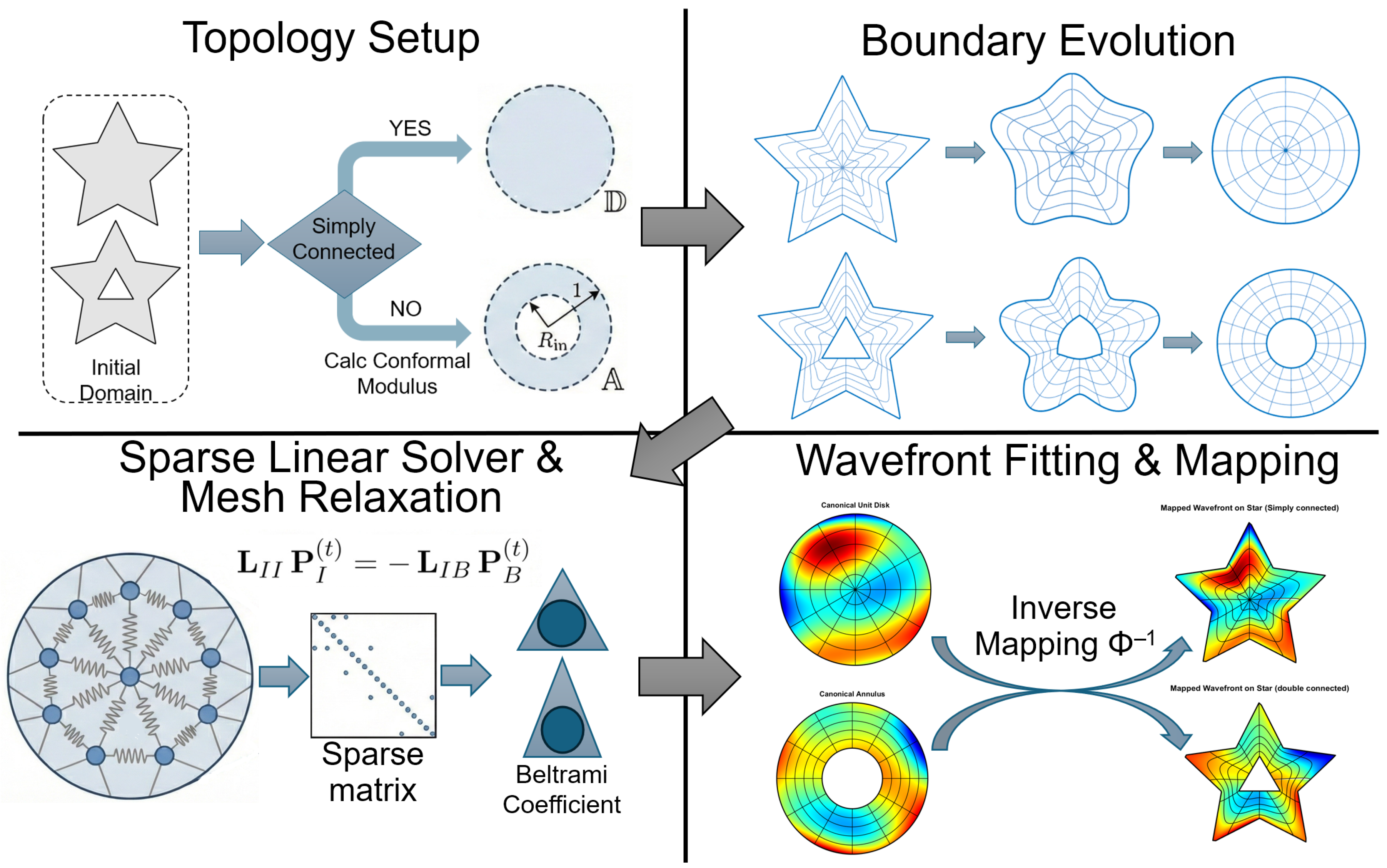
The CSF-QCM pipeline (Figure 1) consists of four distinct steps:

• Boundary geometric regularization (CSF). We evolve the physical boundary $\partial \mathcal{M}$ under discrete curve-shortening flow. This iterative process smooths high-curvature features (e.g., sharp corners of a star-shaped aperture) and generates a sequence of regularized boundary frames that converge to a canonical circle, minimizing grid crowding effects.
• Topology-aware canonical domain specification. The target domain ${\Omega }_{\mathrm{can}}$ is determined by the aperture’s topology. For simply connected domains, ${\Omega }_{\mathrm{can}}$ is set to the unit disk $\mathbb{D}$. For doubly connected domains (e.g., apertures with central obscurations like a triangular hole), we solve the harmonic equation to compute the Dirichlet energy and derive the conformal modulus. This uniquely defines the inner radius $R_{\mathrm{in}}$ of the target annulus $\mathbb{A}$, ensuring a conformal bijection.
• Interior mesh optimization via Laplacian construction. We construct the discrete Laplacian matrix $\mathbf{L}$ using cotangent weights to approximate the harmonic energy. The interior parameterization is obtained by solving the sparse linear system $\mathbf{L}\mathbf{u}=-{\mathbf{L}}_{\mathrm{bd}}{\mathbf{u}}_{\mathrm{bd}}$, where the boundary conditions ${\mathbf{u}}_{\mathrm{bd}}$ are updated progressively using the CSF frames. This step relaxes the internal mesh vertices to minimize angular distortion.
• Wavefront resampling and orthogonal fitting. Using the computed bijection $\Phi$, we map the wavefront data into the canonical domain. Depending on the topology determined in step 2, the wavefront is fitted using standard Zernike polynomials (for disk $\mathbb{D}$) or annular Zernike polynomials (for annulus $\mathbb{A}$), allowing for high-precision reconstruction over arbitrary free-form apertures.

2.3. Boundary Regularization via Curve-Shortening Flow

Conformal maps can be numerically fragile on non-smooth boundaries because corners and sharp curvature variations induce large derivatives and crowding. We therefore smooth the boundary geometry prior to parameterization.

Let $\mathcal{C}(u,t):S^1\times [0,T]\to {\mathbb{R}}^2$ denote a parameterized boundary curve, where t is evolution time and $\mathbf{N}(u,t)$ is the inward unit normal. Under curve-shortening flow (CSF), the boundary evolves by [27]

$${\displaystyle \frac{\partial \mathcal{C}(u,t)}{\partial t}}=\kappa (u,t)\mathbf{N}(u,t),$$

(1)

where $\kappa (u,t)$ is curvature. Intuitively, high-curvature regions move faster, smoothing the curve.

Because CSF ultimately shrinks embedded plane curves to a round point, the evolution must be stopped early. We monitor a circularity deviation metric $E_{\mathrm{circ}}^{\left(k\right)}$ (defined on the discrete boundary at iteration k) and terminate when the relative change is sufficiently small:

$$\left|{\displaystyle \frac{E_{\mathrm{circ}}^{(k+1)}-E_{\mathrm{circ}}^{\left(k\right)}}{E_{\mathrm{circ}}^{\left(k\right)}+\epsilon }}\right|<{ϵ}_{\mathrm{tol}},$$

(2)

where ${ϵ}_{\mathrm{tol}}={10}^{-6}$ and $\epsilon$ is a small constant to avoid division by zero. This criterion indicates that high-frequency boundary irregularities have been sufficiently attenuated while preserving topology.

For doubly connected apertures, the same evolution is applied to both $\partial {\Omega }_{\mathrm{out}}$ and $\partial {\Omega }_{\mathrm{in}}$ (with appropriate inward normals defined with respect to the domain).

2.4. Progressive Strategy

To avoid instability under large deformations, we decompose the mapping into a sequence of small transitions. The intermediate boundary states are provided by the CSF frames. At each frame t, we impose Dirichlet boundary positions on $\partial {\Omega }_{\mathrm{can}}$ and compute interior vertex positions by harmonic relaxation. To ensure mesh robustness and prevent triangle flips, we employ the graph Laplacian [28], denoted by $\mathbf{L}$, which is used here purely as a numerical smoothing operator rather than a geometric Laplace discretization.

The interior coordinates are solved via the linear system:

$${\mathbf{L}}_{II}{\mathbf{P}}_I^{\left(t\right)}=-{\mathbf{L}}_{IB}{\mathbf{P}}_B^{\left(t\right)}$$

(3)

where ${\mathbf{P}}_B^{\left(t\right)}$ stores the fixed boundary vertex coordinates on $\partial {\Omega }_{\mathrm{can}}$, and ${\mathbf{P}}_I^{\left(t\right)}$ stores the unknown interior coordinates. The matrices ${\mathbf{L}}_{II}$ and ${\mathbf{L}}_{IB}$ are the sub-blocks of $\mathbf{L}$ corresponding to the interior (I) and boundary (B) vertex indices, respectively.

The rationale for employing the Laplacian operator lies in its connection to Dirichlet energy minimization. The solution to the harmonic equation $\Delta u=0$ corresponds to the configuration that minimizes the stretching energy of the mapping, analogous to the equilibrium state of a stretched rubber sheet or a spring network.

In our framework, once the boundary geometric tension is released by the CSF evolution, the Laplacian solver naturally propagates this relaxation into the domain interior. By minimizing the local Dirichlet energy, the Laplacian operator promotes smoothness and uniformity in the coordinate field. Rather than prescribing point-to-point matching manually, boundary correspondence is induced by CSF vertex trajectories with arc-length redistribution. This allocates parameter-space resolution to regions that are geometrically difficult (high curvature or near concavities), mitigating the crowding problem typical of static conformal maps.

2.5. Distortion Monitoring and Topological Control

To ensure the topological validity of the mapping throughout the evolution process, we employ the Beltrami coefficient ${\mu }_{\Phi }$ as a rigorous metric for angular distortion. It is defined as Equation (4) [29]:

$${\mu }_{\Phi }\left(z\right)={\displaystyle \frac{\partial \Phi /\partial \overline{z}}{\partial \Phi /\partial z}},{\parallel {\mu }_{\Phi }\parallel }_{\infty }<1.$$

(4)

Mathematically, the condition $\parallel {\mu }_{\Phi }{\parallel }_{\infty }<1$ guarantees that the mapping remains a diffeomorphism, strictly preventing grid folding or overlap.

In our computational framework, $\parallel {\mu }_{\Phi }{\parallel }_{\infty }$ acts as the trigger for an adaptive step-size control mechanism. We enforce a safety threshold $1-ϵ$ (where $ϵ$ is a small margin). During each evolution step, the algorithm performs a tentative update. If the resulting distortion violates the safety condition ($\parallel {\mu }_{\Phi }{\parallel }_{\infty }\ge 1-ϵ$), the update is immediately rejected. Subsequently, the time step is halved ($\delta t\leftarrow \delta t/2$) to reduce the evolution magnitude. This “backtracking” refinement explicitly prevents the solver from overshooting into physically invalid configurations near high-curvature boundaries, thereby robustly preserving the mesh topology.

2.6. Topology-Aware Canonical Annulus for Doubly Connected Domains

For an aperture with an internal obscuration, mapping to the unit disk is topologically invalid [30]. We therefore map to a concentric annulus.

$$\mathbb{A}=\{w\in \mathbb{C}:R_{\mathrm{in}}\le |w|\le 1\}.$$

(5)

The inner radius $R_{\mathrm{in}}$ is determined by the conformal modulus of the physical domain. Assigning an arbitrary radius would introduce significant shear distortion [31].

We compute this conformal invariant by solving a harmonic Dirichlet problem on the physical domain ${\Omega }_{\mathrm{phy}}$ [32,33]:

$$\left\{\begin{array}{cc}\Delta u=0,\hfill & \mathrm{in}{\Omega }_{\mathrm{phy}},\hfill \\ u=0,\hfill & \mathrm{on}\partial {\Omega }_{\mathrm{out}},\hfill \\ u=1,\hfill & \mathrm{on}\partial {\Omega }_{\mathrm{in}}.\hfill \end{array}\right.$$

(6)

On a triangular mesh, we discretize the Laplace–Beltrami operator $\Delta$ using the cotangent weights [34], leading to the stiffness matrix $\mathbf{W}$. We then solve the resulting sparse linear system associated with $\mathrm{W}$ under Dirichlet boundary constraints. The corresponding solution minimizes the Dirichlet energy, defined as follows [35]:

$$E={\int }_{{\Omega }_{\mathrm{phy}}}{\parallel \nabla u\parallel }^2\mathrm{d}\sigma \approx {\mathbf{u}}^{\mathsf{T}}\mathbf{W}\mathbf{u}.$$

(7)

For the canonical annulus, the analytic energy is given by $E=2\pi /ln(1/R_{\mathrm{in}})$. By equating the discrete and analytic energies, we obtain the unique radius:

$$R_{\mathrm{in}}=exp\left(-{\displaystyle \frac{2\pi }{E}}\right).$$

(8)

This ensures the canonical annulus preserves the conformal modulus of the original domain.

2.7. Wavefront Reconstruction and Numerical Stability

After obtaining $\Phi :{\Omega }_{\mathrm{phy}}\to {\Omega }_{\mathrm{can}}$, wavefront samples are mapped as [36]

$$w_i=\Phi (x_i,y_i),W_i=W(x_i,y_i).$$

(9)

We then fit W on the canonical domain using an orthogonal basis.

On $\mathbb{D}$, we use the standard Zernike basis ${\left\{Z_j\right\}}_{j=1}^M$ (Noll indexing) [4]. The expansion is

$$W\approx \sum _{j=1}^M{c}_j{Z}_j\left(w\right),w\in \mathbb{D}.$$

(10)

On $\mathbb{A}$, we use annular Zernike polynomials ${\left\{Z_j^{\mathrm{ann}}(·;R_{\mathrm{in}})\right\}}_{j=1}^M$, which reduce to standard Zernike polynomials as $R_{\mathrm{in}}\to 0$ [37]. The expansion is

$$W\approx \sum _{j=1}^M{c}_j{Z}_j^{\mathrm{ann}}(w;R_{\mathrm{in}}),w\in \mathbb{A}.$$

(11)

With N samples, define the design matrix $\mathbf{H}\in {\mathbb{R}}^{N\times M}$ by

$$H_{ij}={\Psi }_j\left(w_i\right),$$

where ${\Psi }_j$ denotes either $Z_j$ (disk) or $Z_j^{\mathrm{ann}}(·;R_{\mathrm{in}})$ (annulus). The coefficients are obtained by a numerically stable least-squares solve (QR or SVD):

$$\mathbf{c}=\underset{\mathbf{c}\in {\mathbb{R}}^M}{arg\; min}{\parallel \mathbf{H}\mathbf{c}-\mathbf{W}\parallel }_2^2.$$

(12)

In exact arithmetic with continuous uniform sampling, these bases are orthogonal on their canonical domains. In discrete computations, stability is governed by the conditioning of $\mathbf{H}$ (or the Gram matrix $\mathbf{G}={\mathbf{H}}^{\mathsf{T}}\mathbf{H}$). Severe area distortion (high variance of $J_{\Phi }$) effectively introduces non-uniform sampling weights on ${\Omega }_{\mathrm{can}}$, degrading discrete orthogonality and increasing $\kappa \left(\mathbf{H}\right)$ [9]. CSF-QCM leverages bounded quasi-conformal relaxation to mitigate extreme area distortion, thereby improving conditioning and preventing error amplification.

The overall procedure is summarized in Algorithm 1.

Algorithm 1 CSF-Guided Progressive Quasi-Conformal Mapping (CSF-QCM)

Require:  Physical domain mesh ${\Omega }_{\mathrm{phy}}$ with vertices $\mathcal{V}$ and faces $\mathcal{F}$; Wavefront samples vector $\mathbf{W}$; Boundary definition $\partial {\Omega }_{\mathrm{out}}$ (and $\partial {\Omega }_{\mathrm{in}}$ if doubly connected); Tolerance ${ϵ}_{\mathrm{tol}}$.  Ensure:  Canonical mapping $\Phi$, Fitted coefficients $\mathbf{c}$. Step 1: Topology-Aware Target Specification          ▹ See Section 2.6 1: if domain is simply connected then 2:       Set canonical domain ${\Omega }_{\mathrm{can}}\leftarrow \mathbb{D}$ (Unit Disk) 3: else   ▹ Doubly connected case 4:       Solve harmonic Equation (6): $\Delta u=0$ s.t. ${u|}_{\partial {\Omega }_{\mathrm{out}}}{=0,u|}_{\partial {\Omega }_{\mathrm{in}}}=1$ 5:       Compute Dirichlet energy $E\approx {\mathbf{u}}^{\mathsf{T}}\mathbf{W}\mathbf{u}$                  ▹ Equation (7) 6:       Compute conformal modulus: $R_{\mathrm{in}}\leftarrow exp(-2\pi /E)$        ▹ Equation (8) 7:       Set canonical domain ${\Omega }_{\mathrm{can}}\leftarrow \mathbb{A}$ (Annulus with radii $R_{\mathrm{in}},1$) 8: end if Step 2: Boundary Geometric Regularization (CSF)       ▹ See Section 2.3 9: Initialize $k\leftarrow 0$, boundary configuration ${\mathcal{C}}^{\left(0\right)}$ 10: repeat 11:       Compute curvature $\kappa$ and normals $\mathbf{N}$ 12:       Evolve boundary: ${\displaystyle \frac{\partial \mathcal{C}}{\partial t}}\leftarrow \kappa \mathbf{N}$                  ▹ Equation (1) 13:       Update circularity metric $E_{\mathrm{circ}}^{(k+1)}$ 14:       $k\leftarrow k+1$ 15: until Stopping criterion Equation (2) is met: $|\Delta E_{\mathrm{circ}}| <{ϵ}_{\mathrm{tol}}$ 16: Store sequence of boundary frames ${\left\{{\mathcal{C}}^{\left(t\right)}\right\}}_{t=0}^k$ Step 3: Progressive Interior Optimization           ▹ See Section 2.4 17: Construct Graph Laplacian $\mathbf{L}$ 18: Initialize time $t\leftarrow 0$, step size $\delta t$ 19: while $t<T_{\mathrm{end}}$ do                 ▹ Adaptive evolution loop 20:       Evolve boundary candidate: ${\mathcal{C}}_{\mathrm{prop}}\leftarrow {\mathcal{C}}^{\left(t\right)}+\delta t·\left(\kappa \mathbf{N}\right)$ 21:       Update boundary conditions ${\mathbf{P}}_B$ on $\partial {\Omega }_{\mathrm{can}}$ 22:       Solve ${\mathbf{L}}_{II}{\mathbf{P}}_I=-{\mathbf{L}}_{IB}{\mathbf{P}}_B$ for candidate interior ${\mathbf{P}}_{\mathrm{prop}}$ 23:       Compute max distortion ${\mu }_{max}=max{\parallel \mu \left({\mathbf{P}}_{\mathrm{prop}}\right)\parallel }_{\infty }$ 24:       if ${\mu }_{max}<1-ϵ$ then                 ▹ Safety check passed 25:             Accept update: ${\mathcal{C}}^{(t+\delta t)}\leftarrow {\mathcal{C}}_{\mathrm{prop}}$, store mapping frame 26:             $t\leftarrow t+\delta t$ 27:       else                  ▹ Distortion violation detected 28:             Reject update 29:             Reduce step size: $\delta t\leftarrow \delta t/2$           ▹ Adaptive refinement 30:       end if 31: end while 32: Construct final map $\Phi$ Step 4: Wavefront Fitting                   ▹ See Section 2.7 33: Map sample points: $w_i\leftarrow \Phi (x_i,y_i)$ 34: if ${\Omega }_{\mathrm{can}}=\mathbb{D}$  then 35:       Construct $\mathbf{H}$ using Standard Zernike $\left\{Z_j\right\}$           ▹ Equation (10) 36: else 37:       Construct $\mathbf{H}$ using Annular Zernike $\left\{Z_j^{\mathrm{ann}}(·;R_{\mathrm{in}})\right\}$      ▹ Equation (11) 38: end if 39: Solve $\mathbf{c}={arg\; min\parallel \mathbf{H}\mathbf{c}-\mathbf{W}\parallel }_2^2$ via QR/SVD 40: return $\Phi ,\mathbf{c}$

3. Results

We evaluate three representative freeform aperture types exhibiting pronounced geometric challenges, corresponding to specific optical metrology scenarios:

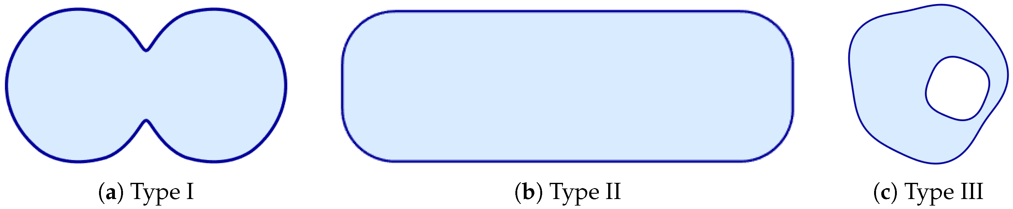
• Type I: A non-convex butterfly-shaped aperture, typical of the irregular interference regions encountered in speckle metrology, as shown in Figure 2a;
• Type II: A high-aspect-ratio rounded rectangle, representing the geometry of primary or secondary mirrors in wide-field-of-view off-axis three-mirror anastigmat (TMA) systems, as shown in Figure 2b;
• Type III: A highly eccentric doubly connected annulus, modeling the pupil in fundus aberration interferometry where the central macular region creates an off-center obscuration, as shown in Figure 2c.

3.1. Mesh Distribution and Sampling Uniformity

In mapping-based wavefront fitting, local cell areas determine discrete quadrature weights and influence numerical stability. Excessive area compression or stretching leads to oversampling or undersampling and degrades least-squares conditioning.

3.1.1. Visual Assessment of Parameterization Meshes

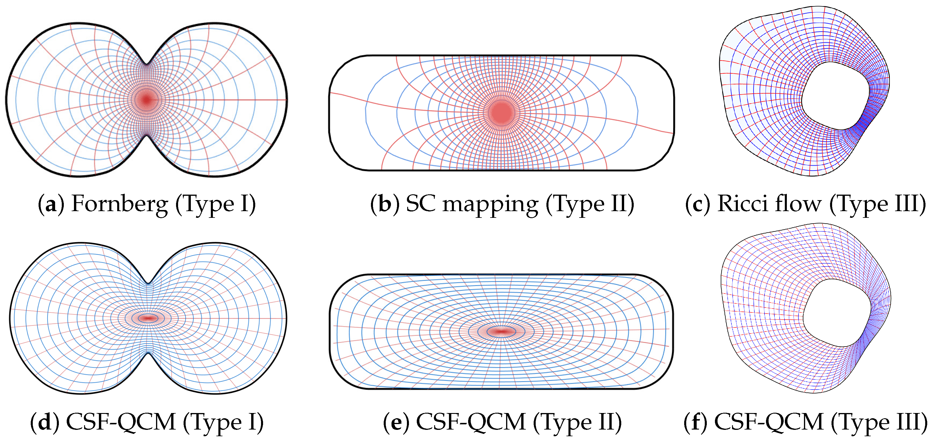
Figure 3 illustrates that strict conformality can impose geometric rigidity, producing highly non-uniform meshes on irregular boundaries:

• Type I (Butterfly): Fornberg-type conformal mapping exhibits strong crowding near concave regions, yielding redundant sampling.
• Type II (Rounded rectangle): Schwarz–Christoffel (SC) mapping compresses the grid near the ends of the long axis due to crowding, producing disproportionate sampling.
• Type III (Annulus): Discrete Ricci flow preserves angles but can introduce severe area distortion in narrow eccentric gaps.

By contrast, CSF-QCM smooths high-frequency boundary features and redistributes arc length during CSF evolution, resulting in quasi-uniform meshes across all cases while preserving topology.

3.1.2. Quantitative Statistics of Area Distortion

To quantitatively evaluate the sampling uniformity, we analyze the statistical distribution of the local area scaling factors. For a mesh $\mathcal{T}={\left\{{\tau }_i\right\}}_{i=1}^N$ generated on the physical domain, the normalized area ratio ${\eta }_i$ for the i-th element is defined as

$${\eta }_i={\displaystyle \frac{\mathrm{Area}\left({\tau }_i\right)}{\overline{A}}},$$

(13)

where $\overline{A}$ is the global average element area. Ideally, for a quasi-uniform sampling, ${\eta }_i$ should be concentrated around 1.

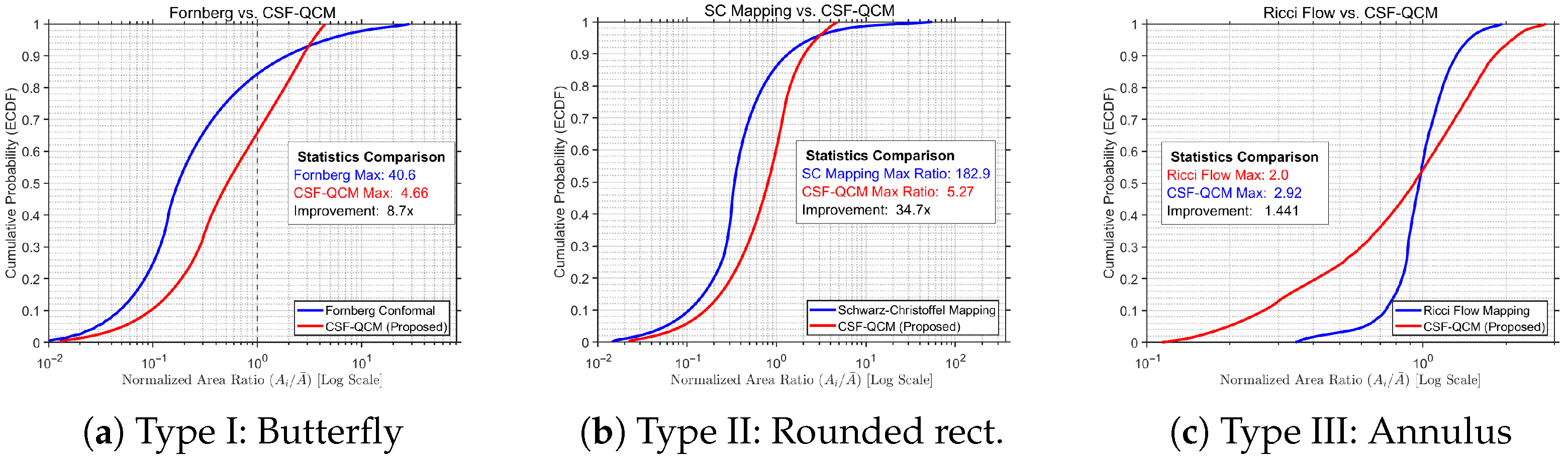
The Empirical Cumulative Distribution Functions (ECDFs) of these ratios are compared in Figure 4. The baseline Fornberg method (blue line) exhibits a broad, sloping distribution with a heavy left tail, indicating that a significant portion of the domain suffers from severe grid compression (crowding) or expansion. In contrast, the CSF-QCM result (red line) rises sharply towards probability 1, forming a steep, step-like profile centered at ${\eta }_i\approx 1$. This geometric characteristic directly evidences that the proposed framework effectively suppresses extreme area variations [16], yielding the homogeneous sampling density required for stable numerical fitting.

3.2. Characterization of Quasi-Conformal Distortion and Discrete Orthogonality

The key mechanism of CSF-QCM is to implicitly accommodate local angular distortion to improve global area uniformity. This section examines the Beltrami coefficient distribution as a post-mapping indicator and the resulting recovery of discrete orthogonality.

3.2.1. Beltrami Coefficient Distribution and Topological Verification

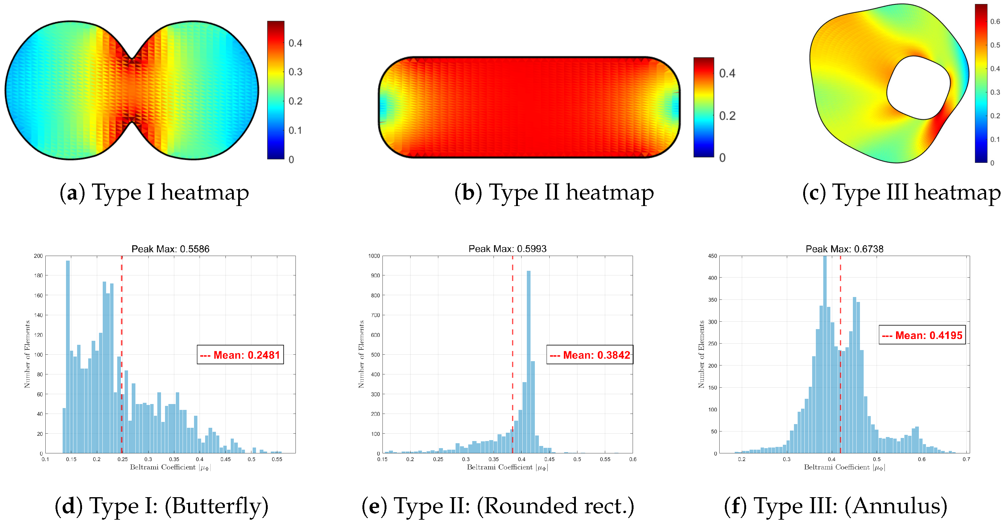
Strict conformality enforces ${\mu }_{\Phi }\equiv 0$ everywhere, a rigid constraint that often necessitates severe area distortion to accommodate irregular boundaries. CSF-QCM relaxes this constraint via progressive quasi-conformal deformation. As illustrated in the spatial maps (Figure 5a–c), moderate $|{\mu }_{\Phi }|$ values are strategically introduced in geometrically constrained regions (e.g., the concave turns in Type I or long-edge endpoints in Type II) to relieve boundary-induced tension.

The statistical histograms in Figure 5d–f provide quantitative verification of the mapping quality:

• Global quasi-conformality. The distributions are heavily skewed towards zero, indicating that the mapping preserves local angles and remains conformal over the vast majority of the domain.
• Topological integrity. The maximum recorded coefficient $\parallel {\mu }_{\Phi }{\parallel }_{\infty }$ remains strictly below the theoretical limit of 1 across all aperture types. This empirically confirms that the adaptive step-size control successfully prevented mesh folding or overlapping, guaranteeing a valid diffeomorphism even at sharp corners.

3.2.2. Recovery of Discrete Orthogonality

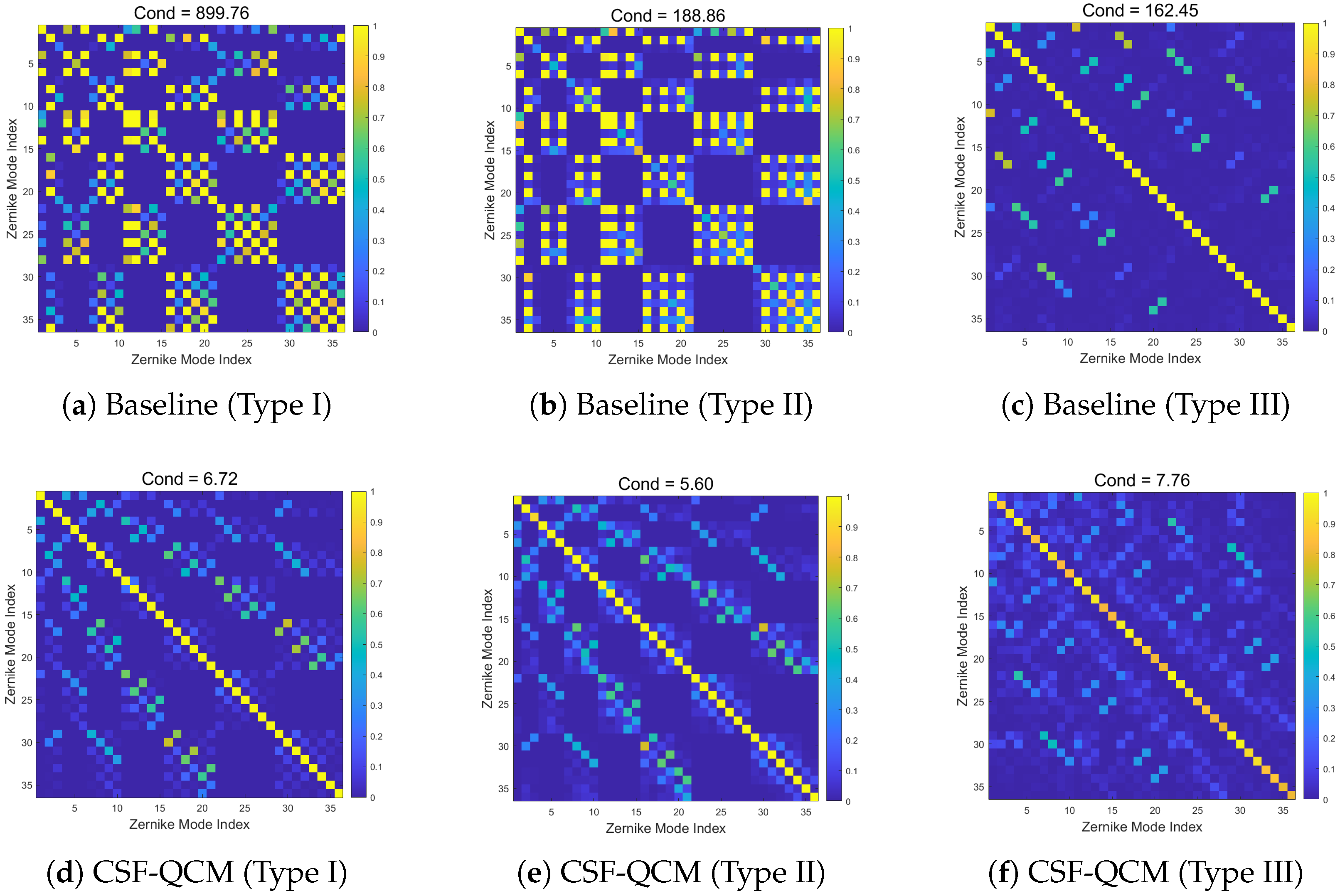
When the mapping $\Phi$ induces highly non-uniform area scaling, the discrete orthogonality of the canonical basis is compromised. This degradation is visualized by the structure of the Gram matrix $\mathbf{G}={\mathbf{H}}^{\mathsf{T}}\mathbf{H}$. In an ideal scenario with uniform sampling, $\mathbf{G}$ should be an identity matrix (up to normalization). However, as shown in the top row of Figure 6, baseline conformal mappings produce Gram matrices with significant off-diagonal components (modal crosstalk), particularly for the high-aspect-ratio Type II and eccentric Type III apertures. This structure indicates that the basis functions have become numerically linearly dependent on the sampled grid, leading to an ill-conditioned inverse problem.

By contrast, CSF-QCM explicitly optimizes for sampling uniformity. As illustrated in the bottom row of Figure 6, the resulting Gram matrices are strictly diagonally dominant with suppressed off-diagonal terms, confirming the recovery of discrete orthogonality. We quantify this improvement using the condition number $\kappa \left(\mathbf{G}\right)$ for the first 36 Zernike modes (

Table 1. Condition number $\kappa \left(\mathbf{G}\right)$ of the Gram matrix (first 36 modes) under different mappings.

Method	Type I	Type II	Type III
	(Butterfly)	(Rounded Rect.)	(Annulus)
Baseline (Fornberg/SC/Ricci)	899.76	188.86	162.45
CSF-QCM (proposed)	6.72	5.60	7.76

). While baseline methods yield condition numbers ranging from ∼162 to over 900, implying amplification of measurement noise, CSF-QCM consistently reduces $\kappa \left(\mathbf{G}\right)$ to single digits (<8) across all aperture types. This near-optimal conditioning ensures that the wavefront fitting remains numerically stable and minimizes the propagation of potential measurement errors.

3.3. Wavefront Fitting Accuracy and Computational Efficiency

To validate the reconstruction fidelity, we generated a synthetic wavefront composed of the first 36 Zernike modes (using Noll indexing for simply connected domains and the corresponding annular basis for Type III), with an RMS amplitude of $1/20\lambda$. This setup mimics typical high-precision testing scenarios where minimizing residual fitting error is critical.

3.3.1. Fitting Error Analysis

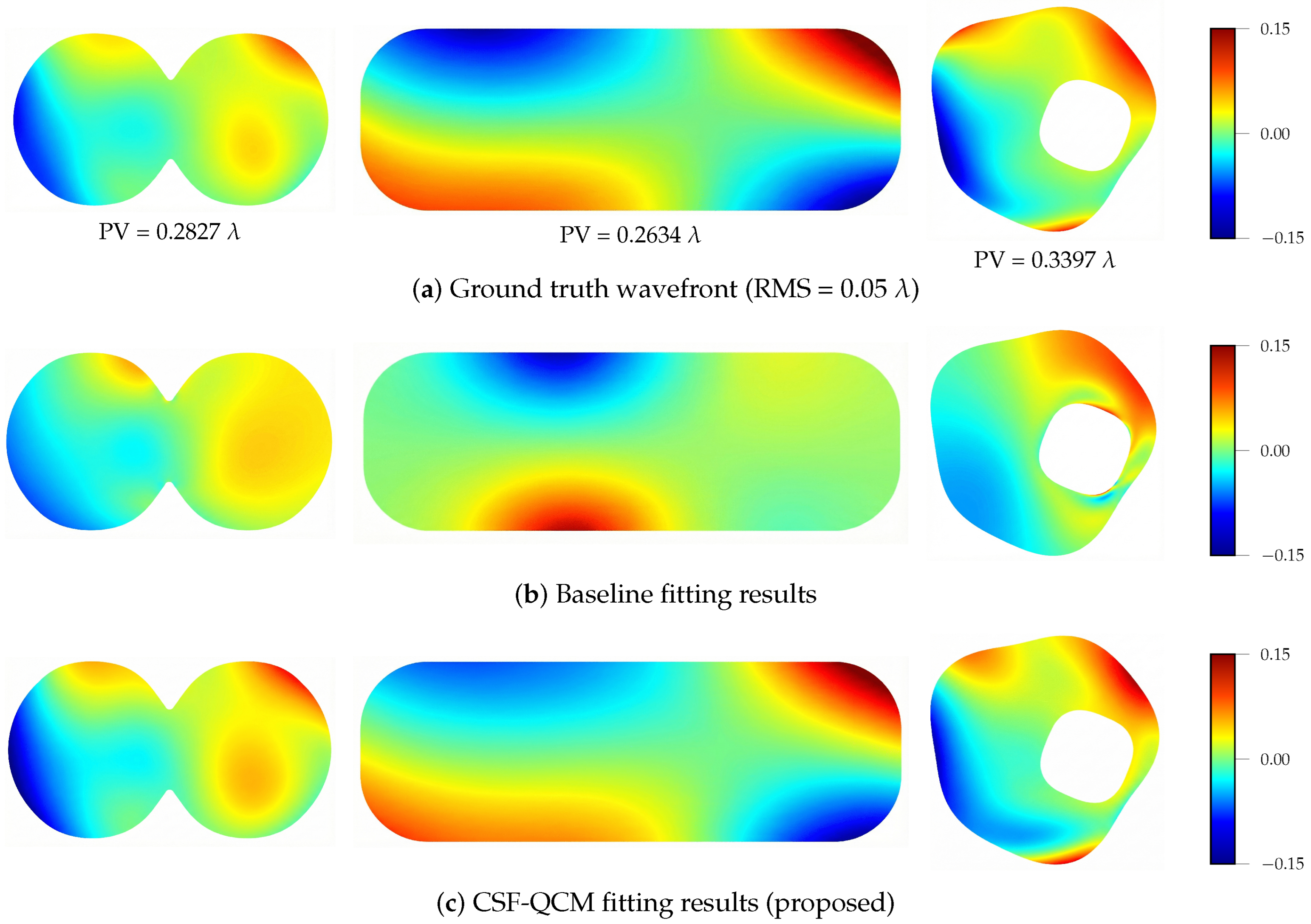
Figure 7 presents a visual comparison of the reconstructed wavefronts against the ground truth. Generally, the baseline methods in Figure 7b capture the global low-frequency aberrations but struggle with local fidelity at the boundaries. This limitation is most physically apparent in the Type II (rounded rectangle) aperture. Due to the high aspect ratio, standard conformal mappings suffer from “exponential crowding” at the longitudinal ends, creating a sampling singularity where the grid density collapses. Consequently, the baseline reconstruction in Figure 7b fails to resolve the wavefront curvature at these extremities, producing visible distortions. In contrast, the CSF-QCM results (Figure 7c) maintain high visual fidelity across all geometries, effectively correcting these boundary artifacts.

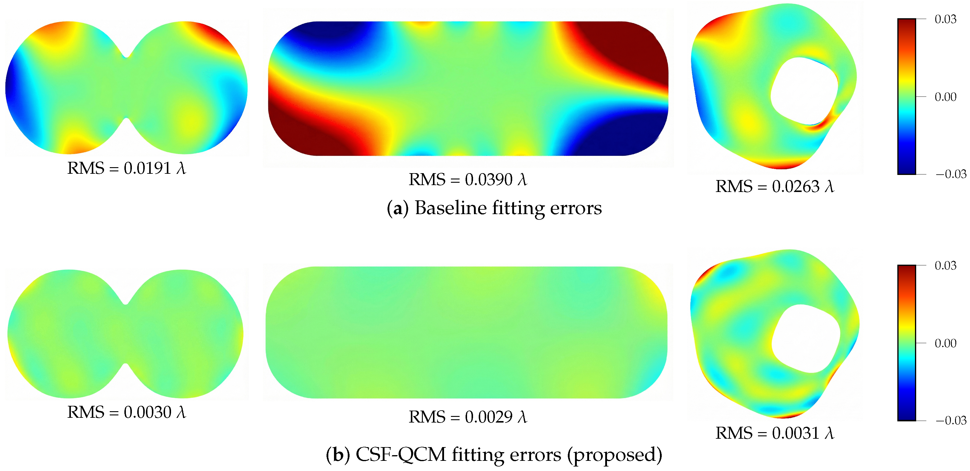
The quantitative advantage of the proposed method is explicitly revealed in the residual error maps (Figure 8). For the baseline approaches (Figure 8a), the errors exhibit a spatially concentrated morphology. Significant “red-blue” oscillating error zones appear near the concave corners of Type I and the narrow ends of Type II, confirming the presence of boundary ringing effects caused by ill-conditioned sampling. Conversely, the CSF-QCM error maps (Figure 8b) demonstrate a spatially homogeneous distribution with negligible magnitude. By introducing controlled quasi-conformal relaxation to relieve mapping tension, the proposed method eliminates these sampling bottlenecks, reducing the RMS error by an order of magnitude (e.g., from $0.0390\lambda$ to $0.0029\lambda$ for Type II).

Table 2. Wavefront reconstruction residuals (PV and RMS in $\lambda$) comparing baselines to CSF-QCM.

Aperture Type	Method	PV Residual		RMS Residual
		Value	Reduction	Value	Reduction
Type I (Butterfly)	Fornberg-type	0.1576	–	0.0191	–
	CSF-QCM	0.0255	83.82%	0.0030	84.3%
Type II (Rounded rect.)	SC mapping	0.2687	–	0.0390	–
	CSF-QCM	0.0392	85.41%	0.0029	92.56%
Type III (Annulus)	Discrete Ricci flow	0.3317	–	0.0263	–
	CSF-QCM	0.0448	86.49%	0.0031	88.21%

quantitatively summarizes the Peak-to-Valley (PV) and Root-Mean-Square (RMS) residuals. Across all three aperture types, CSF-QCM significantly outperforms the baseline approaches. For visible wavelengths (e.g., $\lambda \approx 633$ nm), the method achieves nanometer RMS accuracy. Notably, for the most challenging Type II (rounded rectangle) and Type III (eccentric annulus) apertures, the RMS fitting error is reduced by over 90%, demonstrating the method’s robustness against complex boundary topologies.

3.3.2. Noise Robustness Analysis

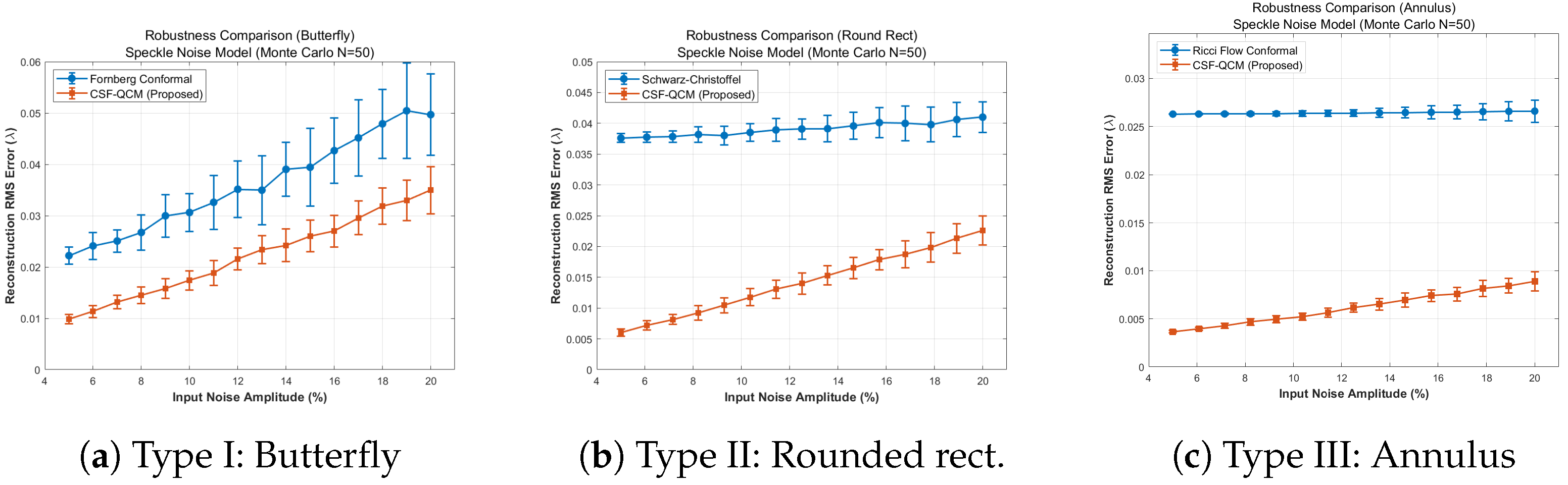
In practical metrology, such as digital holography or speckle interferometry, measurement noise is inevitable. To validate the feasibility of CSF-QCM in realistic scenarios, we performed a Monte Carlo simulation ($N=50$) introducing speckle-type multiplicative noise to the wavefront data. The input noise amplitude was varied from 5% to 20% of the wavefront PV.

Figure 9 compares the reconstruction RMS error trends between the proposed method and the baseline conformal mappings.

The results indicate a fundamental advantage of the proposed framework. Standard conformal mappings (blue lines) exhibit either a high initial error floor (Types II and III) or large variance (Type I) due to the high condition number of their Gram matrices ($\kappa \left(\mathbf{G}\right)>160$), which amplifies the projection of measurement noise onto the Zernike basis. In contrast, CSF-QCM (orange lines) maintains a low condition number ($\kappa \left(\mathbf{G}\right)<8$), ensuring that the reconstruction error remains proportional to the input noise level without numerical amplification. This stability confirms the method’s applicability to experimental data with finite signal-to-noise ratios.

3.3.3. Runtime Analysis

Beyond accuracy, practical metrology demands computational efficiency. We evaluated the runtime on a standard PC (Intel i5 CPU, 16 GB RAM) using meshes with approximately 15,000 vertices.

Table 3. Runtime comparison on typical meshes (∼15,000 vertices). Time unit: seconds.

Aperture Type	Method	Preprocessing	Mapping	Total
Type I	Fornberg	0.25	4.82	5.07
(Butterfly)	CSF-QCM	0.85	1.95	2.80
Type II	SC mapping	0.10	7.45	7.55
(Rounded rect.)	CSF-QCM	0.90	2.10	3.00
Type III	Ricci flow	0.00	8.30	8.30
(Annulus)	CSF-QCM	1.20	2.45	3.65

details the computational cost broken down by processing stage. Although CSF-QCM introduces an iterative boundary evolution step, the total runtime remains competitive (∼3 s). This is achieved because the subsequent interior mapping relies on solving sparse linear systems, which is computationally inexpensive compared to the nonlinear optimization required by Ricci flow. The proposed framework thus offers a favorable trade-off, providing high-precision reconstruction with a computational cost suitable for routine laboratory testing.

4. Discussion

CSF-QCM improves accuracy and numerical stability for wavefront fitting on simply and doubly connected apertures by effectively managing the trade-off between conformality (angle preservation) and area uniformity (sampling regularity). Several aspects merit further investigation.

4.1. Extension to Multiply Connected Apertures

The current framework uses a capacity-based invariant to determine the canonical annulus for doubly connected domains. For more complex topologies (e.g., triply connected apertures, segmented mirrors, or pupils with multiple obscurations), the canonical domain is no longer a simple annulus. Possible extensions include circle-domain parameterizations leveraging fast boundary integral equation methods [38] or analytical approaches based on the Schottky–Klein prime function [39]. These modern numerical tools offer superior convergence rates compared to classical Koebe-type iterative constructions for general n-connected planar domains. CSF-based boundary smoothing remains applicable and can be combined with these multi-boundary canonicalization techniques to handle complex segmented pupil geometries.

4.2. Interaction Between Quasi-Conformal Distortion and Aberration Estimation

The present optimization emphasizes geometric uniformity, while mapping distortion may interact with finite sampling and specific aberration modes. A useful next step is to quantify the sensitivity of estimated coefficients to local quasi-conformal distortion, e.g., through a distortion–aberration sensitivity matrix. Such a model could enable distortion allocation strategies that prioritize regions most influential to the targeted aberration terms, conceptually analogous to the weighted Zernike decomposition strategies employed in high-contrast imaging [40].

4.3. Acceleration Toward Real-Time Metrology

Although CSF-QCM achieves second-level runtime on typical meshes, online metrology may require remeshing and remapping when the valid aperture changes dynamically. The dominant cost arises from large sparse linear solves (Equation (3)). While GPU-accelerated sparse factorizations can reduce latency, a more transformative direction is the adoption of physics-informed machine learning. Specifically, Physics-Informed Neural Networks (PINNs) [41] or Deep Operator Networks (DeepONet) [42] could serve as real-time surrogate models to predict the mapping functions directly by learning the underlying Laplace operator, potentially bypassing the iterative mesh generation process entirely.

5. Conclusions

We presented a CSF-guided progressive quasi-conformal mapping framework (CSF-QCM) to address the loss of orthogonality and numerical instability in wavefront fitting on non-circular freeform apertures. By introducing boundary evolution as a geometric preprocessing step, the framework constructs low-distortion parameterizations from irregular physical apertures—including non-convex, high-aspect-ratio, and doubly connected domains—to canonical computational domains.

The quantitative validations presented in this study highlight three key advancements. Firstly, the numerical stability is drastically improved. By managing the conformality–uniformity trade-off, CSF-QCM reduces the condition number of the Gram matrix from severe levels (e.g., >900 for butterfly apertures) to single digits (<8) across all tested geometries, effectively resolving the ill-conditioning caused by crowding. Secondly, this stability translates into superior reconstruction accuracy. The method eliminates boundary ringing artifacts and achieves nanometer-level precision (RMS $\approx 0.003\lambda$), reducing fitting errors by over 80% (up to 92.5% for high-aspect-ratio shapes) compared to baseline Fornberg and Ricci flow algorithms. Thirdly, the framework maintains computational efficiency, processing typical meshes (∼15 k vertices) in approximately 3 s, which is faster than the iterative Ricci flow and suitable for routine laboratory testing.

In summary, CSF-QCM provides a unified, robust, and fast preprocessing route for wavefront fitting over arbitrary apertures, addressing critical challenges in high-precision freeform metrology and the alignment of complex off-axis optical systems.

References

1. Malacara, D. Optical Shop Testing; John Wiley & Sons: Hoboken, NJ, USA, 2007. [Google Scholar]
2. Ye, J.; Chen, L.; Li, X.; Yuan, Q.; Gao, Z. Review of optical freeform surface representation technique and its application. Opt. Eng. 2017, 56, 110901. [Google Scholar] [CrossRef]
3. Niu, K.; Tian, C. Zernike polynomials and their applications. J. Opt. 2022, 24, 123001. [Google Scholar] [CrossRef]
4. Noll, R.J. Zernike polynomials and atmospheric turbulence. J. Opt. Soc. Am. 1976, 66, 207–211. [Google Scholar] [CrossRef]
5. Zernike, F. Diffraction theory of the knife-edge test and its improved form, the phase-contrast method. Mon. Not. R. Astron. Soc. 1934, 94, 377–384. [Google Scholar] [CrossRef]
6. Galaktionov, I.; Sheldakova, J.; Samarkin, V.; Toporovsky, V.; Kudryashov, A. Atmospheric turbulence with Kolmogorov spectra: Software simulation, real-time reconstruction and compensation by means of adaptive optical system with bimorph and stacked-actuator deformable mirrors. Photonics 2023, 10, 1147. [Google Scholar] [CrossRef]
7. Lee, J.H.; Shin, S.; Park, G.N.; Rhee, H.G.; Yang, H.S. Atmospheric turbulence simulator for adaptive optics evaluation on an optical test bench. Curr. Opt. Photonics 2017, 1, 107–112. [Google Scholar] [CrossRef]
8. Tao, X.; Dean, Z.; Chien, C.; Azucena, O.; Bodington, D.; Kubby, J. Shack-Hartmann wavefront sensing using interferometric focusing of light onto guide-stars. Opt. Express 2013, 21, 31282–31292. [Google Scholar] [CrossRef]
9. Navarro, R.; López, J.L.; Díaz, J.A.; Sinusía, E.P. Generalization of Zernike polynomials for regular portions of circles and ellipses. Opt. Express 2014, 22, 21263–21279. [Google Scholar] [CrossRef] [PubMed]
10. Ferreira, C.; López, J.L.; Navarro, R.; Sinusia, E.P. Orthogonal systems of Zernike type in polygons and polygonal facets. arXiv 2015, arXiv:1506.07396. [Google Scholar] [CrossRef]
11. Ye, J.; Li, X.; Gao, Z.; Wang, S.; Sun, W.; Wang, W.; Yuan, Q. Modal wavefront reconstruction over general shaped aperture by numerical orthogonal polynomials. Opt. Eng. 2015, 54, 034105. [Google Scholar] [CrossRef]
12. Swantner, W.; Chow, W.W. Gram–Schmidt orthonormalization of Zernike polynomials for general aperture shapes. Appl. Opt. 1994, 33, 1832–1837. [Google Scholar] [CrossRef]
13. Chang, L.; Wei, Z.; Shen, W.; Lin, Z. Wavefront fitting of Interferogram with Zernike polynomials based on SVD. In Proceedings of the 2nd International Symposium on Advanced Optical Manufacturing and Testing Technologies: Optical Test and Measurement Technology and Equipment, Xi’an, China, 2–5 November 2005; SPIE: Bellingham, WA, USA, 2006; Volume 6150, pp. 90–95. [Google Scholar]
14. Chai, X.; Zhang, H.; Lin, X.; Zhou, Y.; Yu, Y. Method for orthogonal fitting of arbitrary shaped aperture wavefront and aberration removal. Opt. Eng. 2024, 63, 054112. [Google Scholar] [CrossRef]
15. Zhang, Y.; An, Q.; Yang, M.; Ma, L.; Wang, L. A Review of Wavefront Sensing and Control Based on Data-Driven Methods. Aerospace 2025, 12, 399. [Google Scholar] [CrossRef]
16. Díaz-Elbal, S.; Martínez-Finkelshtein, A.; Ramos-López, D. Sampling patterns for Zernike-like bases in non-standard geometries. Appl. Math. Comput. 2026, 511, 129727. [Google Scholar] [CrossRef]
17. Bos, L.P.; Levenberg, N. On the calculation of approximate Fekete points: The univariate case. Electron. Trans. Numer. Anal. 2008, 30, 377–397. [Google Scholar]
18. Fornberg, B. A numerical method for conformal mappings. SIAM J. Sci. Stat. Comput. 1980, 1, 386–400. [Google Scholar] [CrossRef]
19. DeLillo, T.K.; Elcrat, A.R. A Fornberg-like conformal mapping method for slender regions. J. Comput. Appl. Math. 1993, 46, 49–64. [Google Scholar] [CrossRef]
20. Driscoll, T.A.; Trefethen, L.N. Schwarz-Christoffel Mapping; Cambridge University Press: Cambridge, UK, 2002; Volume 8. [Google Scholar]
21. Yang, D.; Yang, Z.; Zhang, Y. Modal wavefront reconstruction by Schwarz-Christoffel mapping and Zernike circle polynomials for noncircular pupils. Opt. Lasers Eng. 2025, 184, 108643. [Google Scholar] [CrossRef]
22. Trefethen, L.N. Numerical computation of the Schwarz–Christoffel transformation. SIAM J. Sci. Stat. Comput. 1980, 1, 82–102. [Google Scholar] [CrossRef]
23. Jin, M.; Kim, J.; Luo, F.; Gu, X. Discrete surface Ricci flow. IEEE Trans. Vis. Comput. Graph. 2008, 14, 1030–1043. [Google Scholar] [CrossRef]
24. Zeng, W.; Samaras, D.; Gu, D. Ricci flow for 3D shape analysis. IEEE Trans. Pattern Anal. Mach. Intell. 2010, 32, 662–677. [Google Scholar] [CrossRef] [PubMed]
25. Su, Z.; Wang, Y.; Shi, R.; Zeng, W.; Sun, J.; Luo, F.; Gu, X. Optimal mass transport for shape matching and comparison. IEEE Trans. Pattern Anal. Mach. Intell. 2015, 37, 2246–2259. [Google Scholar] [CrossRef]
26. Zeng, W.; Luo, F.; Yau, S.T.; Gu, X.D. Surface quasi-conformal mapping by solving Beltrami equations. In Proceedings of the IMA International Conference on Mathematics of Surfaces, York, UK, 7–9 September 2009; Springer: Berlin/Heidelberg, Germany, 2009; pp. 391–408. [Google Scholar]
27. Gage, M.; Hamilton, R.S. The heat equation shrinking convex plane curves. J. Differ. Geom. 1986, 23, 69–96. [Google Scholar] [CrossRef]
28. Grone, R.; Merris, R.; Sunder, V.S. The Laplacian spectrum of a graph. SIAM J. Matrix Anal. Appl. 1990, 11, 218–238. [Google Scholar] [CrossRef]
29. Astala, K.; Iwaniec, T.; Martin, G. Elliptic Partial Differential Equations and Quasiconformal Mappings in the Plane (PMS-48); Princeton University Press: Princeton, NJ, USA, 2008. [Google Scholar]
30. Conway, J.B. Functions of One Complex Variable II; Springer Science & Business Media: Berlin/Heidelberg, Germany, 2012; Volume 159. [Google Scholar]
31. Forster, O. Lectures on Riemann Surfaces; Springer Science & Business Media: Berlin/Heidelberg, Germany, 2012; Volume 81. [Google Scholar]
32. Nehari, Z. Conformal Mapping; Courier Corporation: North Chelmsford, MA, USA, 2012. [Google Scholar]
33. Hakula, H.; Rasila, A.; Vuorinen, M. Conformal modulus on domains with strong singularities and cusps. arXiv 2015, arXiv:1501.06765. [Google Scholar] [CrossRef]
34. Pinkall, U.; Polthier, K. Computing discrete minimal surfaces and their conjugates. Exp. Math. 1993, 2, 15–36. [Google Scholar] [CrossRef]
35. Iwaniec, T.; Koh, N.T.; Kovalev, L.V.; Onninen, J. Existence of energy-minimal diffeomorphisms between doubly connected domains. Invent. Math. 2011, 186, 667–707. [Google Scholar] [CrossRef]
36. Tyson, R.K.; Frazier, B.W. Principles of Adaptive Optics; CRC Press: Boca Raton, FL, USA, 2022. [Google Scholar]
37. Mahajan, B.V.N. Zernike annular polynomials and optical aberrations of systems with annular pupils. Appl. Opt. 1994, 33, 8125–8127. [Google Scholar] [CrossRef]
38. Nasser, M.M. Fast computation of the circular map. Comput. Methods Funct. Theory 2015, 15, 187–223. [Google Scholar] [CrossRef]
39. Crowdy, D. Solving Problems in Multiply Connected Domains; SIAM: Philadelphia, PA, USA, 2020. [Google Scholar]
40. Allan, G.; Kang, I.; Douglas, E.S.; Barbastathis, G.; Cahoy, K. Deep residual learning for low-order wavefront sensing in high-contrast imaging systems. Opt. Express 2020, 28, 26267–26283. [Google Scholar] [CrossRef]
41. Romanenko, T.; Razgulin, A.; Iroshnikov, N.; Larichev, A. Wavefront Reconstruction by its Slopes via Physics-Informed Neural Networks. Int. Arch. Photogramm. Remote Sens. Spat. Inf. Sci. 2025, 48, 233–240. [Google Scholar] [CrossRef]
42. Zhang, H.; Chen, C.; Li, F.; Cai, J.; Yao, L.; Dong, F.; Wei, Y.; Liu, Y.; Zhang, X.; Zhou, Y.; et al. Single-Pass Wavefront Reconstruction via Depth Heterogeneity Self-Supervised Neural Operator for Turbulence Correction. Laser Photonics Rev. 2025, 19, e00909. [Google Scholar] [CrossRef]
Figure 1. Pipeline of the CSF-QCM framework.
Photonics 13 00095 g001
Figure 2. Benchmark aperture geometries for validation. (a) Type I (butterfly-shaped), (b) Type II (rounded rectangle), and (c) Type III (annulus doubly connected).
Photonics 13 00095 g002
Figure 3. Comparison of parameterization meshes on physical domains. Top row (ac): baseline conformal approaches with visible crowding or stretching. Bottom row (df): CSF-QCM achieves improved global area uniformity.
Photonics 13 00095 g003
Figure 4. Statistical comparison of grid uniformity via Empirical Cumulative Distribution Function (ECDF). The plot shows the cumulative probability of the normalized local area ratio η i = Area ( τ i ) / A ¯ .
Photonics 13 00095 g004
Figure 5. Analysis of Beltrami coefficients. Top row (ac): Spatial distributions of the Beltrami magnitude | μ Φ | for the three aperture types. Bottom row (df): Corresponding statistical histograms. The distribution of | μ Φ | characterizes the degree of quasi-conformal relaxation: non-zero values emerge in particular regions to accommodate the geometry, facilitating global area uniformity while preserving the diffeomorphic property ( | μ Φ |   < 1 ).
Photonics 13 00095 g005
Figure 6. Comparison of Gram matrices G (first 36 Zernike modes). Top row (ac): Baseline approaches (Fornberg, SC, and Ricci flow) exhibit significant off-diagonal energy (crosstalk), indicating loss of orthogonality due to non-uniform sampling. Bottom row (df): CSF-QCM effectively recovers discrete orthogonality, yielding diagonally dominant matrices with significantly reduced condition numbers.
Photonics 13 00095 g006
Figure 7. Comparison of wavefront reconstruction results. (a) Ground truth wavefronts for Type I, II, and III apertures. (b) Reconstructed wavefronts using baseline methods (Fornberg, SC mapping, Ricci flow). (c) Reconstructed wavefronts using the proposed CSF-QCM. While visually similar, the baseline methods in (b) exhibit visible distortions near high-curvature boundaries or ends, which are effectively corrected in (c).
Photonics 13 00095 g007
Figure 8. Visual comparison of residual error maps. (a) Error maps for baseline methods. Significant boundary artifacts (crowding effects) are visible as red/blue zones near concave corners or longitudinal ends. (b) Error maps for the proposed CSF-QCM. Both sets are displayed with the same narrow color scale [ 0.03 λ , 0.03 λ ]. The proposed method achieves an order-of-magnitude reduction in RMS error, maintaining a uniformly low error distribution across all aperture types.
Photonics 13 00095 g008
Figure 9. Robustness comparison under varying speckle noise amplitudes (Monte Carlo N = 50 ). The error bars represent the standard deviation of the RMS reconstruction error. The proposed CSF-QCM (orange) consistently exhibits lower residuals and tighter error spreads compared to baseline conformal methods (blue), which suffer from noise amplification due to ill-conditioning.
Photonics 13 00095 g009