FMCW LiDAR Nonlinearity Compensation Based on Deep Reinforcement Learning with Hybrid Prioritized Experience Replay

Abstract

Frequency-modulated continuous-wave (FMCW) LiDAR systems are extensively utilized in industrial metrology, autonomous navigation, and geospatial sensing due to their high precision and resilience to interference. However, the intrinsic nonlinear dynamics of laser systems introduce significant distortion, adversely affecting measurement accuracy. Although conventional iterative pre-distortion correction methods can effectively mitigate nonlinearities, their long-term reliability is compromised by factors such as temperature-induced drift and component aging, necessitating periodic recalibration. In light of recent advances in artificial intelligence, deep reinforcement learning (DRL) has emerged as a promising approach to adaptive nonlinear compensation. By continuously interacting with the environment, DRL agents can dynamically modify correction strategies to accommodate evolving system behaviors. Nonetheless, existing DRL-based methods often exhibit limited adaptability in rapidly changing nonlinear contexts and are constrained by inefficient uniform experience replay mechanisms that fail to emphasize critical learning samples. To address these limitations, this study proposes an enhanced Soft Actor-Critic (SAC) algorithm incorporating a hybrid prioritized experience replay framework. The prioritization mechanism integrates modulation frequency (MF) error and temporal difference (TD) error, enabling the algorithm to dynamically reconcile short-term nonlinear perturbations with long-term optimization goals. Furthermore, a time-varying delayed experience (TDE) injection strategy is introduced, which adaptively modulates data storage intervals based on the rate of change in modulation frequency error, thereby improving data relevance, enhancing sample diversity, and increasing training efficiency. Experimental validation demonstrates that the proposed method achieves superior convergence speed and stability in nonlinear correction tasks for FMCW LiDAR systems. The residual nonlinearity of the upward and downward frequency sweeps was reduced to $1.869\times {10}^{-5}$ and $1.9411\times {10}^{-5}$, respectively, with a spatial resolution of 0.0203m. These results underscore the effectiveness of the proposed approach in advancing intelligent calibration methodologies for LiDAR systems and highlight its potential for broad application in high-precision measurement domains.

1. Introduction

FMCW LiDAR is a cutting-edge technology for high-precision distance measurement for applications ranging from 3D imaging [1,2] and self-driving [3,4], as well as precision instrument manufacturing and measurement [5,6]. The heart of the FMCW LiDAR system is the linear sweep of the signal, which generates a linear FM optical signal. This signal is split into a reference beam and a detection beam, which interfere after traversing different optical paths. This interference produces a beat frequency that is proportional to the distance to the target, resulting in accurate distance measurements. However, the inherent nonlinearity of the FMCW LiDAR system distorts the linear relationship between the modulating signal and the swept frequency response, leading to the appearance of spectral spreading and measurement errors, as well as the reduction in measurement accuracy, and this nonlinearity is a major bottleneck in the development of high-performance FMCW LiDAR systems.

In FMCW lidar systems, various frequency modulation techniques are employed, depending on the type of light source. These techniques include altering the laser cavity length through periodic mechanical stretching or mirror driving, regulating carrier concentration via current injection, and adjusting the internal cavity temperature through thermal tuning. Common methods for correcting frequency modulation nonlinearity effects include iterative current pre-distortion [7], optical phase-locked loops (OPLLs) and feedback systems [8], equal-frequency resampling [9], and optical frequency comb calibration [10]. However, each method involves limitations. The iterative pre-distortion correction technique combining drive current and time-frequency self-injection locking technology can achieve relative nonlinearity of 100 GHz under a sweeping bandwidth, achieving a wide sweeping range and high linearity with $6.4\times {10}^{-7}$; [11]. However, it also faces drawbacks such as high experimental apparatus and system complexity, the sensitivity of correction results to system feedback parameters, and insufficient long-term stability, requiring frequent recalibration. OPLL systems are complex and expensive. Equal-frequency resampling techniques are bulky and perform poorly for fast-moving targets. Optical frequency comb methods are highly accurate but expensive and require complex hardware configurations. These methods generally lack adaptability to dynamic system conditions and do not support real-time compensation. Therefore, there is an urgent need for new methods to address nonlinearity in frequency sweeping under dynamic conditions. The field of photonics is gradually shifting from traditional physical modeling to data-driven methods, fueled by the increasing availability of simulation and experimental data. This evolution opens new opportunities for applying machine learning to complex photonics challenges. Among these, reinforcement learning (RL) has shown strong potential for optimizing control in nonlinear, time-varying systems. Its effectiveness has been demonstrated in areas such as robotics, autonomous driving, and strategic gaming [12,13,14]. In photonics, RL is emerging in applications like optical microscopy, inverse design, and optical communication. It has been used to enhance ultrafast laser dynamics, stabilize pulse generation, and improve beam quality. In optical communications, RL-based algorithms have been developed to optimize signal modulation and demodulation [15,16,17]. Nevertheless, the application of RL in optical system control, especially in FMCW LiDAR—remains in its infancy, highlighting the need for further exploration in this area.

Recent progress in addressing FMCW LiDAR nonlinearities using reinforcement learning includes model-based control strategies employing actor–critic networks to generate highly linear laser sweeps [18]. Subsequent enhancements have integrated double-critic architectures with delayed policy updates and smoothed regularization to mitigate estimation bias in the critic network, thereby improving chirp control accuracy [19]. Nonetheless, both approaches face notable limitations in continuous control scenarios. Actor–critic frameworks are prone to insufficient exploration, suboptimal convergence, and sensitivity to hyperparameters such as learning rates and update intervals. While the dual-critic design in [19] reduces overestimation bias present in [18], it relies on a fixed exploration noise variance, limiting adaptability to dynamic system behavior. Moreover, excessive policy smoothing may inadvertently hinder effective exploration in complex control environments.

In contrast, the Soft Actor-Critic (SAC) [20] algorithm offers a more robust alternative for correcting laser modulation nonlinearities through a maximum entropy reinforcement learning framework [21]. By jointly optimizing expected return and policy entropy, SAC adaptively generates accurate laser drive signals to compensate for distortions arising from intrinsic laser characteristics and environmental factors like thermal drift. The dual-Q architecture and automatic entropy coefficient adjustment maintain exploratory behavior while enhancing modulation linearity. However, standard SAC implementations still exhibit limitations in FMCW applications: (1) uniform experience sampling and static replay mechanisms struggle to capture critical nonlinear patterns, reducing responsiveness to transient distortions (e.g., startup frequency jumps); (2) fixed delay in data injection fails to account for time-varying disturbances such as rapid temperature shifts; (3) reliance on a single TD error objective neglects hardware-specific observations, thereby constraining adaptability to physical system dynamics. Furthermore, a prioritized experience replay variant of SAC (PER-SAC) has been proposed [22], incorporating a TD-error-based sampling mechanism to emphasize transitions with higher potential for policy improvement. While this approach enhances learning efficiency, it remains suboptimal for FMCW applications. The exclusive reliance on TD error for prioritization overlooks critical physical indicators reflecting hardware state, reducing sensitivity to abrupt nonlinearities. Additionally, fixed-strength importance sampling correction may distort gradient updates for low-priority samples, compromising training stability. Over-sampling high-error experiences can also lead to premature convergence to local optima, which is particularly detrimental in systems requiring ongoing adaptation to changing operational conditions.

To address these issues, this paper proposes an enhanced SAC algorithm called hybrid priority experience replay (HPER). This innovative method achieves a significant leap forward through three key improvements: first, a hybrid priority mechanism based on the modulation frequency error of adjacent modulation segments and TD error is designed, where the dynamic adjustment coefficient is adapted via a Sigmoid function to balance the weights of physical error and strategy error, ensuring a priority response to hardware signals during nonlinear sudden changes while balancing long-term strategy optimization during steady states; second, dynamic importance sampling is introduced, with weighting coefficients automatically matched to the hybrid priority mechanism. This preserves the PER’s deviation correction capability while avoiding training fluctuations caused by over-adjustment. Finally, a time-varying delay injection strategy is innovatively adopted, dynamically adjusting the experience storage rhythm through the real-time monitoring of MF change rates. This shortens delays during rapid nonlinear changes to enhance timeliness and extends delays during stable phases to ensure data diversity. These multi-level improvements enable HPER-SAC to demonstrate significant advantages in FMCW nonlinear correction: an improved response speed to transient distortions and enhanced correction stability under continuous action variations, while maintaining the excellent exploration capabilities of traditional SAC.

The remainder of this paper is organized as follows: Section II describes the principles of FMCW LiDAR and the reinforcement learning network model proposed in this paper. Section III presents the experimental results and discussion, including network parameter settings and experimental result comparisons. Section IV discusses the significance of the research findings and summarizes this paper.

2. Methodology

2.1. FMCW LiDAR Non-Linearity

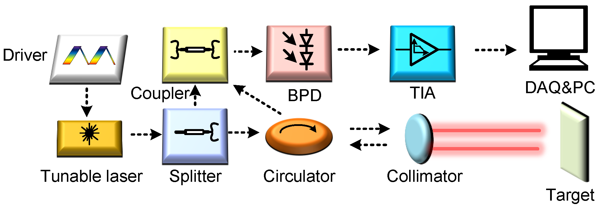
The fundamental architecture of the FMCW LiDAR system is illustrated in Figure 1, which presents a block diagram of a direct detection-based laser ranging configuration. In this system, a triangular waveform generated by a driver modulates a tunable laser source, producing a continuous-wave optical signal with a periodically swept frequency. The emitted light is split into two paths: the measurement beam, directed toward the target via a circulator, and the reference (local) beam, sent to an optical coupler. The measurement beam is collimated, transmitted to the target, and the reflected signal is re-collimated and guided back through the circulator to the coupler. There, it interferes with the local beam, and the resulting optical interference is detected via a balanced photodetector (BPD), which converts it into an electrical beat frequency signal. This signal is then amplified via a trans-impedance amplifier (TIA). The target distance is determined by analyzing the frequency of the beat signal.

External-cavity semiconductor frequency-modulated lasers, which achieve modulation by driving cavity mirrors to vary the optical path length, are widely adopted due to their superior FM linearity, wavelength stability, narrow linewidth, low noise, high side-mode suppression ratio, elevated output power, and compact integration. Despite these advantages, practical implementation is challenged by nonlinearities arising from piezoelectric actuator (PZT) hysteresis, mechanical vibrations, and circuit noise. These effects distort the frequency sweep, introducing errors in the beat frequency $f_b$ and thereby degrading ranging resolution and accuracy. As depicted in Figure 2, the dashed line illustrates the ideal linear frequency modulation trajectory, while the solid line represents the actual, non-ideal modulation behavior encountered in real-world scenarios.

In the range of laser modulation period $(0,T)$, the modulated signal of local light and measure light $f_{LO}\left(t\right)$$f_{me}\left(t\right)$ can be written as follows:

$$\left\{\begin{array}{c}{f}_{lo}\left(t\right)=f_0+kt\hfill \\ f_{me}\left(t\right)=f_0+k(t-{\tau }_d)\hfill \end{array}\right.$$

(1)

Let $f_0$ denote the initial optical frequency and k the modulation rate, defined as $k={\displaystyle \frac{2B}{T}}$, where B represents the laser’s frequency sweep bandwidth and T the modulation period. The parameter ${\tau }_d$ corresponds to the round-trip propagation delay associated with a target located at the target’s distance R, and it is given as follows:

$$R=c{\tau }_d/2$$

(2)

When considering the nonlinear term $f_e\left(t\right)$ of the FMCW LiDAR system, the above Equation (1) can be written as follows:

$$\left\{\begin{array}{c}{f}_{lo}\left(t\right)=f_0+kt+f_e\left(t\right)\hfill \\ f_{me}\left(t\right)=f_0+k(t-{\tau }_d)+f_e\left(t\right)\hfill \end{array}\right.$$

(3)

To calculate the beat frequency, we first need to obtain the phase of the local light and measure light:

$$\left\{\begin{array}{c}{\phi }_{lo}\left(t\right)=2\pi {\int }_0^{t}f\left(v\right)dv=2\pi f_{0}t+\pi k{t}^2+{\int }_0^{t}2\pi f_e\left(t\right)dt+{\phi }_0\hfill \\ {\phi }_{me}\left(t\right)=2\pi f_0\left(t-{\tau }_d\right)+\pi k{\left(t-{\tau }_d\right)}^2+\hfill \\ {\int }_0^{t-{\tau }_d}2\pi f_e\left(t-{\tau }_d\right)dt+{\phi }_0\hfill \end{array}\right.$$

(4)

Then, the phase difference between the measured light signal and the local light signal from Equation (4) can be expressed as follows:

$${\phi }_{lo}\left(t\right)-{\phi }_{me}\left(t\right)=2\pi f_0{\tau }_d+2\pi kt{\tau }_d-\pi k{\tau }_d^2+{\int }_{t-{\tau }_d}^{t}2\pi f_e\left(t\right)dt$$

(5)

Since practical ranging scenarios typically occur within 300 m, the round-trip time ${\tau }_d$ is at most 2$us$. Given that the modulation period T of FMCW LiDAR is generally around 100$us$, we have ${\tau }_d\ll T$. Therefore, we neglect the term ${\tau }_d^2$, $f_e\left(t\right)$ is considered invariant in ${\tau }_d$, and we can get ${\int }_{t-{\tau }_d}^t{f}_e\left(t\right)dt=f_e\left(t\right){\tau }_d$.

Thus, according to Equation (5), the nonlinearity beat signal can be expressed as follows:

$$f_{bn}={\displaystyle \frac{d({\phi }_{lo}\left(t\right)-{\phi }_{me}\left(t\right))}{dt}}=k{\tau }_d+{\displaystyle \frac{d{f}_e\left(t\right)}{dt}}{\tau }_d$$

(6)

And the distance R of the target can be rewritten as follows:

$$R={\displaystyle \frac{c{f}_{bn}}{2k}}={\displaystyle \frac{c{\tau }_d}{2k}}(k+{\displaystyle \frac{d{f}_e\left(t\right)}{dt}})$$

(7)

The accuracy of the beat signal frequency directly determines the precision and resolution of distance measurements in FMCW LiDAR. The ranging resolution is defined as $R_{\mathrm{res}}={\displaystyle \frac{c}{2B}}$. When a window function is applied to the beat signal spectrum via Fourier transform [23], the theoretical spatial resolution (TSR) corresponds to the full width at half maximum (FWHM) of the spectral peak, given by $R_{FWHM}=2R_{\mathrm{res}}={\displaystyle \frac{c}{B}}$. To evaluate the deviation in beat signal frequency $f_{bn}$ introduced via modulation nonlinearity, the bandwidth is estimated using Carson’s rule [24].

$$\delta f_{bn}=2(1+\beta )f_r$$

(8)

where $f_r$ is the repetition of FMCW LiDAR modulation signal, $\beta$ is the modulation index, and has $\beta =2\pi {\tau }_d{f}_{e,rms}$ and $f_{e,rms}$ is the root mean square(RMS) value of nonlinear error. Thus, Equation (8) can be rewritten as $\delta f_{bn}=(1+2\pi {\tau }_d{f}_{e,rms})f_r$. In this way, by analyzing the spectrum of the beat signal, we are able to quantitatively evaluate the sweep nonlinearity, and the $R_{FWHM}$ can be rewritten as [19]:

$$R_{FWHM}={\displaystyle \frac{c(1+2\pi {\tau }_d{f}_{e,rms})}{2B}}$$

(9)

Since we can control the magnitude of the modulation slope $k_c$ to achieve the compensation purpose, the beat frequency by compensation $f_{bn\_c}$ can be expressed as follows:

$$f_{bn\_c}=k_c{\tau }_d+{\displaystyle \frac{d{f}_e\left(t\right)}{dt}}{\tau }_d$$

(10)

The compensated distance $R_c$ can be expressed as follows:

$$R_c={\displaystyle \frac{c{\tau }_d}{2k}}(k_c+{\displaystyle \frac{d{f}_e\left(t\right)}{dt}})$$

(11)

To establish the reinforcement learning environment, we adopt the methodology presented in [19]. The environment is constructed using experimentally obtained data and the underlying principles of FMCW LiDAR measurement. A nonlinear setting is simulated by incorporating Gaussian noise, effectively emulating the real-world nonlinear behavior of FMCW systems. This approach enables efficient policy training without direct interaction with the physical hardware, thereby mitigating the risk of potential damage to laser components. The first step involves formulating the physical relationship between the beat frequency and the modulation slope:

$$f_b\left(t\right)=h\left({\nu }^{\prime }\left(t\right)\right)=h\left(k_c\left(t\right)\right)$$

(12)

The $h(·)$ denotes the Hilbert transform, and $f_b\left(t\right)$ can also be expressed as follows: $f_b\left(t\right)=\mathcal{F}\left(\nu \left(t\right)\right)k_c\left(t\right)$, with $\mathcal{F}(·)$ denoting the nonlinear characteristic. The noise term $n\left(t\right)$ is then introduced to model the stochastic properties of the system:

$$f_{mb}\left(t\right)=\mathcal{F}\left(\nu \left(t\right)\right)k_c\left(t\right)+n\left(t\right)$$

(13)

Based on the given $k_c\left(t\right)$, the modulated beat frequency $f_{mb}\left(t\right)$ is calculated, and the model is constructed as a training environment for the RL algorithm through this relation.

2.2. Soft Actor–Critic with Hybrid Prioritized Experience Replay

The Soft Actor–Critic (SAC) algorithm represents a state-of-the-art reinforcement learning approach founded on the principle of maximum entropy policy optimization. Unlike conventional methods that primarily enhance policy performance through Q-value estimation of a given policy $\pi$, SAC employs a dual-stage optimization process involving both the value and policy functions. This design eliminates the reliance on manually tuned exploration noise parameters, which are often associated with inefficient and unstable policy learning. A distinguishing feature of SAC is its incorporation of an adaptive temperature coefficient, $\alpha$, which is dynamically optimized as part of the objective function. This mechanism obviates the need for manual hyperparameter adjustment, thereby enhancing the algorithm’s ability to adapt to varying environmental complexities and different phases of the training process. Additionally, entropy regularization encourages broader exploration across the state–action space while suppressing redundant interactions with less informative regions. This exploratory efficiency renders SAC particularly well-suited to environments that demand a balance between exploration and learning stability. Despite these advantages, SAC exhibits limitations due to its uniform sampling strategy, which treats all experience samples with equal priority. This can lead to slower convergence and instability during training. To address these issues, prioritized experience replay is introduced into the SAC framework. By emphasizing samples with higher value function estimation errors and suboptimal policy outcomes, the network is guided to focus on experiences with greater learning potential. This modification enhances both the stability and convergence rate of the learning process. The SAC algorithm can be formally described as a policy search within the framework of a Markov decision process (MDP). By extending the standard reward maximization objective with a maximum entropy component, the algorithm aims to jointly maximize the expected return and the entropy of the policy. The resulting policy objective, $J\left(\pi \right)$, is given as follows:

$$J\left(\pi \right)=\sum _t\mathbb{E}[r(s_t,a_t)+\alpha H\left(\pi (·|s_t)\right)]$$

(14)

In this context, $r(s_t,a_t)$ represents the immediate reward received from the environment when the agent is in state $s_t$ and executes action $a_t$ and can be expressed as $r(s_t,a_t)=-norm\left(\right|f_{mb}\left(t\right)-f_{ideal}\left|\right)$ in this paper. The term $H\left(\pi (·|s_t)\right)$ denotes the entropy of the action distribution under policy $\pi$, given state $s_t$, which quantifies the level of randomness in the agent’s action selection at that state. A higher entropy indicates a more exploratory policy. The coefficient $\alpha$ regulates the contribution of the entropy term. The SAC algorithm consists of two primary components: policy evaluation and policy improvement. In the policy evaluation phase, the soft Q-value function, denoted as $Q_{\mathrm{s}}(s_t,a_t)$, is defined as follows:

$$Q_{\mathrm{s}}\left(s_t,a_t\right)=r(s_t,a_t)+\gamma \mathbb{E}\left[V_{\mathrm{s}}\left(s_{t+1}\right)\right]$$

(15)

where $\gamma$ is the discount factor, and the soft state value function $V_{\mathrm{s}}\left(s_t\right)$ is defined as follows:

$$V_{\mathrm{s}}\left(s_{t+1}\right)=\mathbb{E}\left[Q_{\mathrm{s}}\left(s_{t+1},a_{t+1}\right)\right]-\alpha \log \pi \left(a_{t+1}\right|s_{t+1})$$

(16)

The term $\mathbb{E}\left[Q_{\mathrm{s}}\left(s_{t+1},a_{t+1}\right)\right]$ represents the expected soft Q-value obtained by selecting an action according to the current policy in state $s_{t+1}$, capturing the anticipated return following the agent’s decision. The entropy regularization component, $\alpha \log \pi (a_{t+1}\mid s_{t+1})$, promotes stochasticity in the policy by penalizing certainty, thereby encouraging exploration. The temperature parameter $\alpha$ modulates this term, balancing exploration and exploitation by scaling the entropy contribution. Importantly, $\alpha$ is updated adaptively to optimize the trade-off between reward maximization and entropy. This adjustment follows the gradient update rule:

$${\alpha }^{\prime }=\alpha -{\lambda }_{\alpha }{\nabla }_{\alpha }J\left(\alpha \right)$$

(17)

where $\alpha$ and ${\alpha }^{\prime }$ denote the current and updated temperature coefficients, respectively, ${\lambda }_{\alpha }$ is the learning rate, and ${\nabla }_{\alpha }J\left(\alpha \right)$ is the gradient of the entropy-related objective with respect to $\alpha$.

$${\nabla }_{\alpha }J\left(\alpha \right)=-{\displaystyle \frac{1}{N}}\sum (\alpha ·(log\pi +h)$$

(18)

where N denotes the size of the batch data sampled from the empirical playback buffer and h is the target entropy. In the strategy enhancement stage, we optimize the strategy using Kullback–Leibler Divergence [25]:

$${\pi }_{\mathrm{new}}=\mathrm{argmin}(D_{\mathrm{KL}}({\pi }^{\prime }(·|s_t)\Vert {\displaystyle \frac{exp\left(Q^{{\pi }_{\mathrm{old}}}(s_t,·)\right)}{Z^{{\pi }_{\mathrm{old}}}\left(s_t\right)}}))$$

(19)

where $Z^{{\pi }_{\mathrm{old}}}\left(s_t\right)$ is a normalized distributional function, and the output of the strategy ${\pi }_{\phi }$ is a probability distribution. The soft Q-function $Q_{\theta }({\mathrm{s}}_t,{\mathrm{a}}_t)$ parameters can be trained to minimize the soft Bellman residual:

$$J_{Q_{\mathrm{s}}}\left(\theta \right)={\mathbb{E}}_{(s_t,a_t)}\left[{\displaystyle \frac{1}{2}}{(Q_{\theta }(s_t,a_t)-(r(s_t,a_t)+\gamma {\mathbb{E}}_{s_{t+1}}\left[V_{\overline{\theta }}\left(s_{t+1}\right)\right]))}^2\right]$$

(20)

Here, $V_{\overline{\theta }}\left({\mathrm{s}}_{t+1}\right)=\mathbb{E}[Q_{\overline{\theta }}({\mathrm{s}}_{t+1},a_{t+1})-\alpha \log \pi (a_{t+1}\mid {\mathrm{s}}_{t+1})]$, and $Q_{\overline{\theta }}(s_t,a_t)$ denotes the target Q-value network obtained via the exponential moving average of the parameter $\theta$ of the Q-value function for the parameter $\overline{\theta }$. The soft actor–critic algorithm uses the reparameterization trick to redefine the strategy ${\pi }_{\phi }$ as follows:

$$a_t=f_{\phi }({\epsilon }_t;s_t)$$

(21)

where ${\epsilon }_t$ is a random variable in the heavy parameter skill. According to the above definition, the updated gradient of the soft Q function is

$$\begin{array}{cc}\hfill {\nabla }_{\theta }{J}_{Q_{\mathrm{s}}}\left(\theta \right)& ={\nabla }_{\theta }{Q}_{\theta }(a_t,s_t)\left(Q_{\theta }(a_t,s_t)-r(s_t,a_t)\right.\hfill \\ & -\gamma \left(Q_{\theta }(a_{t+1},s_{t+1})-\alpha \log \left({\pi }_{\phi }\left(a_{t+1}\right|s_{t+1})\right)\right)\hfill \end{array}$$

(22)

where $\theta$ and $\overline{\theta }$ are parameters of the soft Q function and its target network, respectively, and the update gradient of the policy network ${\pi }_{\phi }$ is

$${\nabla }_{\phi }{J}_{\pi }\left(\phi \right)=\begin{array}{cc}\hfill & \left({\nabla }_{a_t}log{\pi }_{\phi }(a_t,s_t)-{\nabla }_{a_t}Q(a_t,s_t)\right){\nabla }_{\phi }{f}_{\phi }({\epsilon }_t;s_t)+\hfill \\ \hfill & {\nabla }_{\phi }log{\pi }_{\phi }(a_t,s_t)\hfill \end{array}$$

(23)

During SAC training, experience batches are uniformly sampled from the replay buffer, assigning equal selection probability to all transitions. However, this uniform approach may be suboptimal, as experiences vary in their contribution to learning. Prioritized experience replay addresses this issue by assigning higher sampling probabilities to transitions with greater learning potential, thereby focusing updates on more informative experiences. PER quantifies the importance of each transition using the temporal-difference (TD) error $\delta$, which measures the discrepancy between predicted and actual returns. Larger TD errors indicate transitions with greater potential to improve the policy, and thus, they are prioritized during sampling. The sampling probability for each experience is derived from its TD error, ensuring that data with higher learning relevance are revisited more frequently, thereby improving training efficiency and accelerating convergence. The sampling probability is calculated using the following formulation:

$$P\left(i\right)={\displaystyle \frac{p_i^{{\alpha }_p}}{{\sum }_k{p}_k^{{\alpha }_p}}}$$

(24)

where $p_i$ refers to the priority of state transition, which is a positive number, like $p_i>0$. ${\alpha }_p$ is an exponential hyperparameter corresponding to the priority level to be used and can be regarded as a trade-off factor to balance the uniformity and greediness. When ${\alpha }_p=0$, uniform sampling is performed, and when ${\alpha }_p=1$, greedy (maximum value selection) sampling is performed. However, considering that, in FMCW LiDAR, the global estimate of the TD error representation strategy cannot directly reflect the nonlinear correction results in terms of laser device physics, to ensure accurate correction at the hardware level, we introduce the modulation frequency (MF) difference between the beat frequency signals of adjacent beat frequency units as a feature quantity that directly reflects instantaneous nonlinearity. This enables the integration of MF error and TD error into a hybrid priority mechanism, resolving the compatibility between instantaneous response and long-term optimization for intelligent agents. This achieves a more robust training strategy. The definition of MF error is

$${\delta }_{MF}=|\Delta f_{mb}^{\left(i\right)}|$$

(25)

where $\Delta f_{mb}^{\left(i\right)}$ denotes the difference between the beat frequencies of two adjacent segments of the modulation signal, and the sampling probability $P_{mix}\left(i\right)$ of the new hybrid priority mechanism is

$$P_{mix}\left(i\right)={\displaystyle \frac{({\delta }_{MF}{\left(i\right)}^{ϵ}·|{\delta }_{TD}\left(i\right){{|}^{1-ϵ})}^{{\alpha }_p}}{{\sum }_j({\delta }_{MF}{\left(j\right)}^{ϵ}·|{\delta }_{TD}\left(j\right){{|}^{1-ϵ})}^{{\alpha }_p}}}$$

(26)

Here, $ϵ\in [0,1]$ denotes the mixing coefficient. By setting $ϵ$, the weight ratio between ${\delta }_{TD}$ and ${\delta }_{MF}$ can be dynamically adjusted. And ${\delta }_{TD}$ denotes the TD error, which can be expressed as follows:

$$\begin{array}{cc}\hfill {\delta }_{TD}\left(i\right)=& {\displaystyle \frac{1}{2}}\left(\left|Q_{{\theta }_1}(s_i,a_i)-Q_s(s_i,a_i)\right|\right.\hfill \\ \hfill & \left.+\left|Q_{{\theta }_2}(s_i,a_i)-Q_s(s_i,a_i)\right|\right)\hfill \end{array}$$

(27)

Among them, $Q_{{\theta }_1}(s_i,a_i)$ and $Q_{{\theta }_2}(s_i,a_i)$ are the two value networks of SAC. To further eliminate priority bias, we introduce a dynamic mixing coefficient $\mu$ to control the weights of ${\delta }_{MF}$ and ${\delta }_{TD}$ in the priority, and the importance sampling weight $w\left(i\right)$ can be expressed as follows:

$$w_i={\left({\displaystyle \frac{1}{\left|\mathcal{D}\right|·P_{mix}\left(i\right)}}\right)}^{1-\mu }$$

(28)

When $\mu \approx 1$, $w_i\approx 1$, indicating that ${\delta }_{MF}$ dominates the weighting. When $\mu \approx 0$, $w_i\approx {\displaystyle \frac{1}{\left|\mathcal{D}\right|·P_{mix}\left(i\right)}}$, indicating that ${\delta }_{TD}$ dominates the weighting. The calculation method for $\mu$ is as follows:

$$\mu =\sigma (-{\displaystyle \frac{d\widehat{{\delta }_{MF}}}{dt}})$$

(29)

where $\sigma$ is the sigmoid function, which is defined on [0,1], and $\widehat{{\delta }_{MF}}$ is calculated through the following equation:

$$\widehat{{\delta }_{MF}}={\displaystyle \frac{1}{W}}\sum _{k=t-W+1}^t{\delta }_{MF}\left(k\right)$$

(30)

In FMCW LiDAR systems, the modulation nonlinearity of the laser is influenced by environmental factors like temperature fluctuations and laser degradation, as well as hardware characteristics like driver circuit latency, leading to time-varying behavior. Conventional experience replay (ER) strategies, which typically rely on fixed-delay or immediate data injection, are insufficient for capturing these dynamic nonlinearities. This can result in an imbalance between data recency and diversity, thereby hindering model performance. To address this limitation, we introduce a Time-Varying Delay Experience (TDE) infusion mechanism, which dynamically adjusts the injection delay of training samples based on system dynamics. Combined with buffer segmentation management, this approach ensures a more balanced temporal distribution of experiences. The delay function $\xi \left(t\right)$ is designed to reflect the rate of change in system nonlinearity, modeled using the first-order derivative of the modulation frequency error ${\displaystyle \frac{d{\delta }_{MF}}{dt}}$.

$$\xi \left(t\right)={\xi }_{\mathrm{base}}·\left(1+tanh\left(\eta ·{\displaystyle \frac{d{\delta }_{MF}}{dt}}\right)\right)$$

(31)

where ${\xi }_{\mathrm{base}}$ is the base delay step to ensure minimum data diversity. $\eta$ is the sensitivity coefficient, which controls the strength of the response of the delay to the rate of nonlinear change. The value range of $tanh(·)$ is $[-1,1]$, so the actual range of $\xi \left(t\right)$ is $\xi \left(t\right)\in [0,2{\xi }_{\mathrm{base}}]$, and ${\displaystyle \frac{d{\delta }_{MF}}{dt}}$ is calculated by sliding the modulation frequency error window:

$${\displaystyle \frac{d{\delta }_{MF}}{dt}}\approx {\displaystyle \frac{1}{W}}\sum _{k=t-W+1}^t({\delta }_{MF}\left(k\right)-{\delta }_{MF}(k-1))$$

(32)

where k denotes the current training step, and W represents the window width used to smooth instantaneous noise, typically determined based on the total number of steps in a single training session. When ${\displaystyle \frac{d{\delta }_{MF}}{dt}}>0$, it indicates that the nonlinearity of the modulation signal is intensifying, and the modulation frequency error is increasing rapidly (e.g., sudden rise in laser temperature causing frequency modulation distortion). In this case, $tanh(·)$ approaches 1, $\xi \left(t\right)\approx 2{\xi }_{\mathrm{base}}$, and the delay increases. At this point, the system requires more time to accumulate new data in order to fully capture the evolving trend of nonlinear dynamics. When ${\displaystyle \frac{d{\delta }_{MF}}{dt}}\approx 0$, it indicates that the nonlinearity of the modulation signal is stable, $tanh\left(·\right)\approx 0$, and the base delay is maintained to preserve exploration diversity. When ${\displaystyle \frac{d{\delta }_{MF}}{dt}}<0$, it indicates that the nonlinear trend of the modulation signal is decreasing, the modulation frequency error is decreasing, approaching -1, and $\xi \left(t\right)\approx 0$. At this point, the delay is minimized, and the system needs to quickly inject new data to promptly reflect the nonlinear compensation effect and avoid training lag. In addition, we divide the ER buffer ${\mathcal{D}}_s$ into two sub-buffers, namely the fast zone $D_f$ and the slow zone $D_s$, where the fast zone is used to store experiences in the high dynamic change phase $({\displaystyle \frac{d{\delta }_{MF}}{dt}}>0)$, accounting for $\psi$ of the total capacity, and the slow zone is used to store experiences in the steady state phase $({\displaystyle \frac{d{\delta }_{MF}}{dt}}\le 0)$, with a capacity ratio of $1-\psi$, as shown in the following equation:

$$\left\{\begin{array}{cc}{\mathcal{D}}_f\leftarrow \left(s_t,a_t,r_t,s_{t+1}\right),\hfill & \mathrm{if}{\displaystyle \frac{d{\delta }_{MF}}{dt}}>0\hfill \\ {\mathcal{D}}_s\leftarrow \left(s_t,a_t,r_t,s_{t+1}\right),\hfill & \mathrm{otherwise}\hfill \end{array}\right.$$

(33)

Finally, during sampling, we mixed the two types of data proportionally in batch $\mathcal{B}$ during network training to balance detection and exploitation:

$$\mathcal{B}=\psi ·Sample\left({\mathcal{D}}_f\right)+(1-\psi )·Sample\left({\mathcal{D}}_s\right)$$

(34)

The structure of HPER-SAC is shown in Figure 3. First, the FMCW LiDAR experimental system section, where an Field-Programmable Gate Array (FPGA) generates the original modulated signal, which is then converted into a drive signal via a digital-to-analog converter (DAC) to drive a tunable laser to generate laser light. The laser light is split by a coupler into 10% local light and 90% measurement light. The measurement light then passes through a time-delay fiber before entering a second coupler simultaneously with the local light, where they are mixed and frequency-converted into beat signals via a BPD. Then, an analog-to-digital converter (ADC) quantizes and collects the beat frequency signal to the FPGA. The FPGA transmits the digitized beat frequency data and the original modulation signal to the laptop via a network protocol and initializes the system environment required for RL training. Then, the HPER-SAC reinforcement learning network algorithm is started. First, the actor interacts with the environment and stores the samples in the experience replay buffer. Then, it calculates the beat frequency MF and TD error between adjacent segments within the sweep frequency period to construct a mixed priority experience pool and automatically adjust the proportion of replayed experiences. After training the agent, probabilistic sampling is performed from the experience replay buffer, and the parameters of the critic network are updated. Simultaneously, the target network undergoes a soft update to guide the Actor network in updating the signal modulation actions. The specific HPER-SAC algorithm steps are shown in Algorithm 1.

Algorithm 1 HPER-SAC RL.

Input: Hyperparameters: exponential moving average $\tau$, discount factor $\gamma$, target entropy h, batch size $\mathcal{B}$, Critic NN learning rate ${\lambda }_Q$, Actor NN learning rate ${\lambda }_{\pi }$, entropy coefficient learning rate ${\lambda }_{\alpha }$. Initialize Critic NN: $Q_{{\theta }_1}$, $Q_{{\theta }_2}$; Actor NN: ${\pi }_{\phi }$; Target NN: ${\theta }_1^{\prime }\leftarrow {\theta }_1,{\theta }_2^{\prime }\leftarrow {\theta }_2,{\phi }^{\prime }\leftarrow \phi$. Replay buffer: ${\mathcal{D}}_f$ and ${\mathcal{D}}_s$. for$episode$ = 1 to N, do:      Get initial state $s_1$ and initialize modulation slope $k_c\left(1\right)$.      for $step$ = 1 to T do:         Sample ${\pi }_{\phi }$ by $s_t$ to obtain action $a_t$ and calculate $r_t$ and $s_{t+1}$         Update modulation slope: $k_c\left(t+1\right)\leftarrow a_t$         Store tuple $\left(s_t,a_t,r_t,s_{t+1}\right)$ to $\mathcal{D}$ and calculate ${\delta }_{MF}$, ${\delta }_{TD}$, ${\displaystyle \frac{d{\delta }_{MF}}{dt}}$, $\xi \left(t\right)$         if t mod $\xi \left(t\right)$ == 0:             if ${\displaystyle \frac{d{\delta }_{MF}}{dt}}>0$:               Store tuple $\left(s_t,a_t,r_t,s_{t+1},{\delta }_{TD},{\delta }_{MF}\right)$ to ${\mathcal{D}}_f$             else               Store tuple $\left(s_t,a_t,r_t,s_{t+1},{\delta }_{TD},{\delta }_{MF}\right)$ to ${\mathcal{D}}_s$             end if         end if             Calculate $\mu$, sample a batch transition from ${\mathcal{D}}_f$ to ${\mathcal{B}}_f$, and from ${\mathcal{D}}_s$ to ${\mathcal{B}}_s$, then get $\mathcal{B}$         for $i\in \mathcal{B}$ do:             Calculate $P_{mix}\left(i\right)$ and $w_i$.         end for         Update critic NN loss function: ${\theta }_k\leftarrow {\theta }_k-{\nabla }_{{\theta }_k}\left[{\sum }_i{w}_i{(Q_{{\theta }_k}(s_i,a_i)-y_i)}^2\right](fork\in (1,2))$         Update actor NN loss function: $\phi \leftarrow \phi -{\nabla }_{\phi }\left[{\sum }_i(\mu {\delta }_{MF}+(1-\mu ){\delta }_{TD})\right]$      end for         Update critic networks: ${\theta }_k\leftarrow {\theta }_k-{\lambda }_Q{\nabla }_{{\theta }_k}{J}_{Q_{\mathrm{s}}}\left({\theta }_k\right)(fork\in (1,2))$;         Update actor network: $\phi \leftarrow \phi -{\lambda }_{\pi }{\nabla }_{\phi }{J}_{\pi }\left(\phi \right)$         Update temperature coefficient:$\alpha \leftarrow \alpha -{\lambda }_{\alpha }{\nabla }_{\alpha }J\left(\alpha \right)$         Update target networks: ${\overline{\theta }}_1\leftarrow \tau {\theta }_1+(1-\tau ){\overline{\theta }}_1$; ${\overline{\theta }}_2\leftarrow \tau {\theta }_2+(1-\tau ){\overline{\theta }}_2$. end for Output: control policy

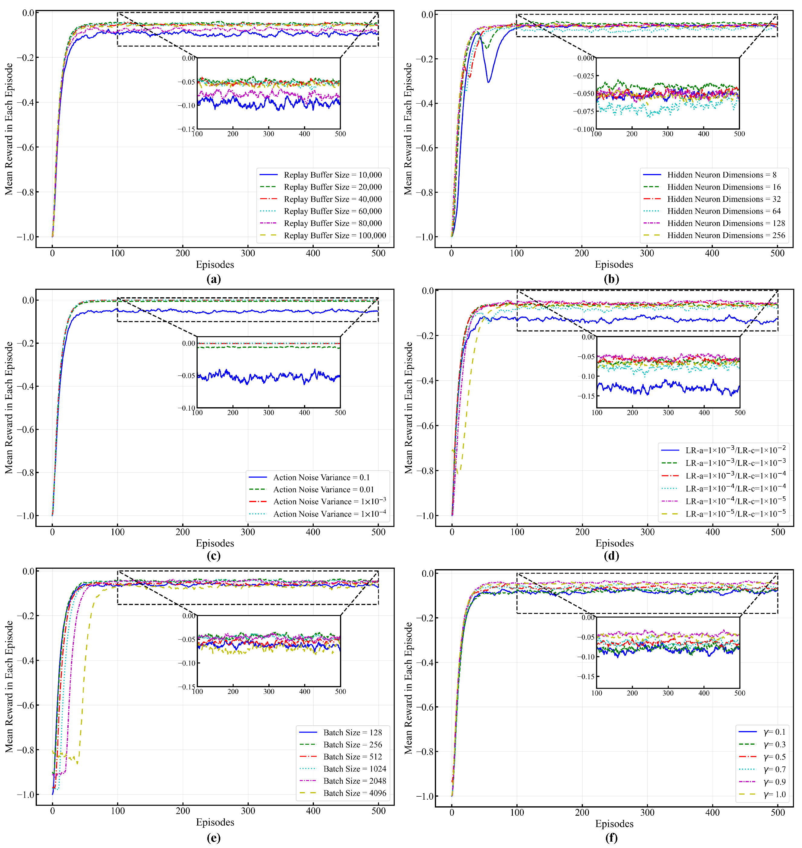
The training parameters are listed in

Table 1. Hyper-parameters setting.

Parameters	Value
Episodes	500
Time steps	100
Batch size	128
Replay buffer size	10,000
Actor NN learning rate	0.01
Critic NN learning rate	0.01
Action noise variance	0.01
Hidden neurons	256
Target entropy	−1
Entropy coefficient learning rate	0.02
Base delay step	1
Sensitivity coefficient	0.5
Exponential moving average	0.005

.

3. Results and Discussion

To validate the proposed method, an experimental FMCW LiDAR system was constructed. The setup employs a tunable laser (PHX-C-T-M-C58-32-6-2-0-0, PHOTONX, Shenzhen, China) operating at a central wavelength of 1550 nm with an average output power of approximately 20 mW. A triangular modulation signal $u\left(t\right)$, superimposed on a DC bias, is used to drive the laser, with a modulation frequency $f_k=10$ kHz (period T = 100 $\mathsf{\mu }$s) and a sweep bandwidth of 12 GHz. The AD9238 (ADC, 65 MSPS, 12 bit, Analog Devices, Inc., Norwood, MA, USA) and AD9767(DAC, 125 MSPS, 14 bit, Analog Devices, Inc., Norwood, MA, USA) are employed as sampling and quantizing beat-to-beat signals and generating analog modulation signals. We conducted reinforcement learning training on a laptop running the Windows 10 operating system, using Python 3.8.20 and the PyTorch 2.5.0 environment. The CPU is a Ryzen 7 5800H (Advanced Micro Devices, Inc., Santa Clara, CA, USA) with a base clock speed of 3.19 GHz, the GPU is a GeForce RTX 3060 (NVIDIA, Inc., Santa Clara, CA, USA), and the system has 6 GB of RAM.

3.1. Training Parameters Optimization

As shown in Figure 4a, the reward curve exhibits the highest instability when the replay buffer size is limited to 10,000. This is primarily due to reduced sample diversity and the loss of critical exploratory transitions, particularly in environments with high nonlinearity. These conditions increase the risk of convergence to suboptimal policies and amplify update variance, leading to significant reward oscillations. While increasing buffer size enhances stability, sizes beyond 60,000–80,000 degrade performance and increase resource consumption, thereby reducing data efficiency [18]. A buffer size of 40,000 provides an effective balance between stability and computational efficiency. Figure 4b analyzes the effect of hidden layer size. Smaller sizes (8, 16, 32) result in greater early-stage reward variance and slower convergence. However, increasing the size to 64 degrades both stability and performance. A hidden layer size of 128 achieves the most stable convergence, with reward values stabilizing near −0.05, indicating it is the optimal configuration. In Figure 4c, the influence of action noise variance is examined. A variance of 0.1 leads to the highest reward instability and poor convergence. Lower variances, such as 0.01, improve convergence speed but reduce exploration, increasing the risk of local optima. Thus, careful tuning of noise variance is essential to balance exploration and exploitation. Figure 4d explores the impact of learning rates. Larger rates for policy and value networks (e.g., LR-a = 1 $\times {10}^{-3}$, LR-c = 1 $\times {10}^{-2}$) induce greater reward fluctuations and lower final performance. Conversely, very small rates (e.g., LR-a = LR-c = 1 $\times {10}^{-5}$) yield higher rewards but also cause instability. Both extremes compromise convergence and learning efficiency, necessitating moderate learning rate selection. The batch size also significantly influences model performance, particularly in capturing latent environmental structures. Larger batch sizes improve training stability but increase computational cost. As shown in Figure 4e, batch sizes above 2048 slow early exploration and delay convergence, while smaller sizes (e.g., 128) accelerate learning but result in high reward variance. A batch size of 256 offers a suitable trade-off. Finally, Figure 4f highlights the role of the discount factor $\gamma$. Values near 1 emphasize long-term returns, facilitating global policy optimization, whereas lower values favor short-term rewards, increasing the likelihood of suboptimal convergence. In FMCW LiDAR, where nonlinearity evolves over time and cumulative effects are critical, short-term focus is insufficient. While $\gamma =1$ introduces instability due to sensitivity to small action changes, a moderate value of $\gamma =0.8$ achieves stable and effective learning.

Then, we evaluated the training performance of six algorithms: the standard actor-critic method, the model-based reinforcement learning approach from Ref. [18], the twin-critic actor-critic method from Ref. [19], the original SAC, the prioritized experience replay SAC (PER-SAC), and the proposed hybrid prioritized experience replay SAC (HPER-SAC). As illustrated in Figure 5, the optimized HPER-SAC algorithm demonstrates clear advantages over the others in terms of maximum achieved reward, convergence speed, and stability, thereby validating its effectiveness.

3.2. Experiment Evaluation Based on Different RL Algorithms

To assess the effectiveness of nonlinear compensation on the beat-frequency signal, experiments were conducted using an FMCW LiDAR system at a distance of 1m. Based on Equations (11) and (12), the theoretical beat frequency under ideal, linear conditions is approximately 1.6 MHz. As shown in Figure 6, the HPER-SAC algorithm produces a beat-frequency spectrum with noticeably sharper peaks than other correction methods. This reflects reduced spectral dispersion, fewer spurious components, improved spatial resolution, and lower frequency deviation, demonstrating the method’s superior capability in correcting nonlinear distortions.

To evaluate the stable nonlinear correction effect and resolution of the FMCW laser, we need to monitor the long-term performance stability of the nonlinear correction method and its adaptability to laser performance degradation to assess the reliability of this model in practical applications. The FMCW LiDAR nonlinear correction experimental system operated continuously for over 2 h, updating the correction results every hour under constant parameters, and the root mean square (RMS) value of nonlinear error $f_{e,rms}$ was used to evaluate the stability of nonlinear correction. We also compared the stability of correction effects from other methods, as shown in Figure 7. It can be observed that, with the accumulation of time, the relative $f_{e,rms}$ value exhibits the greatest variability in the 55–68 MHz range for the ActorCritic algorithm, while the variability ranges for the methods in [18,19] are approximately 50 MHz and 40 MHz, respectively. The fluctuations of the SAC and PER-SAC algorithms both fall within the range of 40–50 MHz. Finally, the proposed HPER-SAC algorithm exhibits the smallest fluctuation range at around 15 MHz. Therefore, after the correction results are compared over an extended period, our proposed method demonstrates a significant stability advantage over other methods.

And furthermore, in order to verify the improvement of the spatial resolution of the beat signal after correction, we calculated the $f_{e,rms}\left(t\right)$ of the beat signal after correction and the theoretical spatial resolution (TSR) according to Equations (13) and (14), respectively, and compared them with the methods in other references.

As shown in

Table 2. Nonlinear compensation evaluation of different methods at 1m@($f_b$ = 1.6 MHz).

Method	Beat Signal Bandwidth (kHz)	${\mathit{f}}_{\mathit{e},\mathbf{rms}}$ (MHz)	TSR (m)
Actor-Critic	71.43	61.421	0.0446
[18]	62.5	50.756	0.0391
[19]	55.56	42.468	0.0347
SAC	50	35.828	0.0312
PER-SAC	47.62	32.985	0.0298
HPER-SAC	32.54	14.976	0.0203

, under the same test environment, by correcting the nonlinearity of FMCW LiDAR, the method proposed in this paper achieves a beat frequency signal bandwidth of 40 kHz, while other methods, such as ordinary Actor-Critic, references [18,19], and single SAC, PER-SAC achieve beat frequency signal bandwidths ranging from 47.62 kHz to 71.43 kHz, reducing the bandwidth by 54.4%, 47.9%, 41.4%, 34.9%, and 31.7%, respectively. A lower bandwidth indicates fewer signal components in other frequency bands caused by nonlinearity, more concentrated energy in the main lobe signal, and higher spectral resolution of the main signal. After calculating the RMS of the nonlinear residuals $f_{e,rms}$, our proposed method achieved a reduction of 54.6% to 75.6% compared to the other five methods, indicating that our method has a significant advantage in terms of nonlinear correction effectiveness. Finally, at a test distance of 1.6m, a theoretical spatial resolution of 0.0203 m was achieved, representing an improvement of 31.9% to 54.5% compared to the other methods.

Furthermore, we evaluate the system residual nonlinearity of different methods by calculating the $(1-r^2)$ [24], which can be expressed as follows:

$$1-r^2=12{(f_{e,rms}/B)}^2$$

(35)

The outcome of up sweep and down sweep of FMCW laser after compensation are plotted in Figure 8c and Figure 8d, respectively. At the same time, in order to compare with the nonlinear correction results, we also present the original uncorrected laser sweep results. In Figure 8, the orange curve indicates the frequency variation of light sweep, and the blue curve represents the residual error, which means the difference between the actual frequency and the ideal frequency. The indicators $f_{e,rms}$ and $(1-r^2)$ directly reflect the frequency linearity of the sweep light. The $f_{e,rms}$ of up and down sweep light are 14.976 MHz and 15.262 MHz. The indicator $(1-r^2)$ of them are $1.869\times {10}^{-5}$ and $1.9411\times {10}^{-5}$. The smaller these two parameters are, the higher the linearity of the FMCW laser sweep.

Furthermore, to validate the effectiveness of our method on different lasers, we conducted test experiments using a new continuous tunable laser (TSL-SWT-M-C-20-P-FA, realphoton, Inc., Shenzhen, China) and conducted experimental tests, as shown in Figure 9. The laser was driven by a 10 kHz repetition rate modulation signal, achieving a modulation bandwidth of 10 GHz. The final $f_{e,rms}$ values for the up and down sweep light were 12.36 MHz and 11.86 MHz, respectively. The linearity indicator $(1-r^2)$ for these values are $1.273\times {10}^{-5}$ and $1.172\times {10}^{-5}$, demonstrating slightly improved linearity compared to previous lasers.

A comparative analysis was conducted to assess the calibration performance of various methods over 100 repeated measurements at test distances of 1 m, 3 m, 7 m, and 9 m. The resulting distance distributions were visualized using box plots, as shown in Figure 10. The results indicate that the proposed HPER-SAC algorithm yields smaller deviations between the maximum and minimum measured values and the ground truth across all tested distances, relative to other approaches. Furthermore, the box plots corresponding to the HPER-SAC method exhibit shorter interquartile ranges and median values that are more closely aligned with the theoretical distances. These findings suggest that the proposed method achieves lower variance, tighter data dispersion, and more consistent calibration performance compared to the benchmark techniques.

Finally, we present the FPGA hardware resources used in the entire RL agent training and actual beat frequency signal correction application, including ADC module and DAC module drivers and data register comprehensive layout, as well as the LUT (Look-Up Table), FF (Flip-Flop), BRAM (Block Random Access Memory), IO (Input/Output), BUFG (Global Clock Buffer), MMCM (Mixed-Mode Clock Manager), and other resources used. These are shown in

Table 3. Resource consumption of FPGA when applying RL trained model.

Parameter Type	Resource Usage
LUT	2773
FF	3045
BRAM	2
IO	63
BUFG	5
MMCM	2

below.

4. Conclusions

This study proposes a hybrid priority experience replay soft actor–critic algorithm to address the nonlinear correction challenge in FMCW LiDAR systems. The proposed method innovatively combines the exploration advantage of maximum entropy reinforcement learning with a hybrid experience replay mechanism, achieving a significant improvement in LiDAR compensation performance. By introducing a priority scheme that combines nonlinear modulation frequency error priority in adjacent segments with time difference error-based strategy priority, the algorithm achieves parallel optimization of hardware characteristics and control strategies. Based on a dynamic importance sampling mechanism, the sampling weights are adaptively adjusted according to the hybrid priority scheme, thereby enhancing training stability and efficiency. Subsequently, a time-varying delay data injection strategy is employed to dynamically adjust the data storage intervals based on nonlinear dynamics, simultaneously improving temporal correlation and sampling diversity. The experimental results show that in the task of source nonlinearity correction for FMCW LiDAR, our proposed method has obvious advantages over other methods in the literature in terms of measurement accuracy, spatial resolution, and residual nonlinearity, which will provide a basis for realizing higher-performance FMCW LiDAR system in the future.