Abstract
The solution of the Helmholtz equation describing the propagation of light in free space from a plane to another can be described by the angular spectrum operator, which acts in the frequency domain. Many applications require this operator to be generalized to handle tilted source and target planes, which has led to research investigating the implications of these adaptations. However, the frequency domain representation intrinsically limits the understanding the way the signal is transformed through propagation. Instead, studying how the operator maps the space–frequency components of the wavefield provides essential information that is not available in the frequency domain. In this work, we highlight and exploit the deep relation between wave optics and quantum mechanics to explicitly describe the symplectic action of the tilted angular spectrum in phase space, using mathematical tools that have proven their efficiency for quantum particle physics. These derivations lead to new algorithms that open unprecedented perspectives in various domains involving the propagation of coherent light.
1. Introduction
In monochromatic wave optics, light propagation is usually modelled as an integral operator providing a solution to the Helmholtz equation between two parallel planes, i.e., deriving the value of the field in one plane knowing its value in a shifted one []. When it comes to non-parallel planes, a convenient way to extend the solution to Helmholtz equation is by using the angular spectrum expression of the propagation operator. The study of the adaptations to be brought to this operator for handling tilted planes was first conducted by Matsushima [], which has since been successfully used in practical optics applications [] and remains to be the reference formulation in the frequency domain to this day. However, for many applications, namely related to hologram generation, compression and adaptive display, it is required to work in the so-called phase space, i.e., the space–frequency domain [,]. Indeed, the representations of holograms in the space or frequency domains are highly chaotic, and a semantically meaningful regularity can only be exhibited through phase space transformations such as wavelets, windowed Fourier transform, Gabor frames or Wigner–Ville distribution [].
An interesting approach to obtain a formulation of tilted propagation in phase space is given by the mathematical tools of quantum mechanics. It is a well-established fact that monochromatic wave propagation shares a mathematical framework with quantum mechanics [,]. In fact, quantum mechanics has been historically guided by the strong parallel between optics and mechanics []. Indeed, wave optics appears as the equivalent of “quantizing” geometrical optics. It is thus not surprising that optics results can be obtained by applying mathematical theories that have been developed for better understanding quantum mechanics, such as semiclassical analysis and microlocal analysis []. In particular, these theories provide an extensive study of integral operators—of which propagation operators appear as special cases—that can be interpreted as quantized versions of phase space transformations called symplectomorphisms in mathematics and canonical transformations in physics.
While this theoretical similarity is known in the semiclassical community, this in-depth understanding of near-classic behaviour is rarely exploited in optics; the phase space treatment is usually restricted to the linear symplectomorphisms [,] or empirical displacements of coefficients []. Although the time evolution operators in phase space have been successfully applied to various domains in previous works [,,], to the best of our knowledge, no study has been carried for expressing the tilted angular spectrum on space–frequency expansions.
In this paper, we use symplectic techniques to derive the expression of propagation on tilted planes in phase space. More explicitly, we exhibit the symplectomorphism associated with the modified operator mentioned in [] and show how it can be used on some common space–frequency representations. Although restricting our derivations to the first order of approximation (i.e., geometric optics completed with adequate phase factors), our study introduces the semiclassical concepts and sets a framework for investigating wave-specific phenomena described by higher-order terms.
The rest of the paper is organized as follows: In Section 2, we review the basic symplectic tools that are needed to derive the targeted formulas. In Section 3, we use these principles to obtain the recipe allowing us to extract the wanted symplectomorphism from the integral operator of tilted angular spectrum. In Section 4, this recipe is applied to obtain the phase space symplectomorphism that we break up in Section 5 in order to extract finer information. In Section 6, we apply this symplectomorphism to various space–frequency distributions in order to simulate tilted propagation in phase space. Finally, we present simulations and visual results in Section 7.
2. Overview of Considered Symplectic Techniques
In this section, we provide a very short overview of the semiclassical and microlocal analysis results that are used in the rest of this paper. These domains are extremely vast, as is symplectic geometry, the mathematical theory dealing with the natural transformations of physical phase spaces; hence, we will only cite the relevant results for our purpose, and provide links for the reader unfamiliar with these domains to possibly obtain a deeper understanding of the theory. In particular, this section can be skipped by the reader only interested in computational aspects.
It is well known [] that wave optics and quantum mechanics share the same mathematical formulation. In fact, the historical derivation of the Schrödinger equation, which describes the evolution of the wave function, has been inspired by the similarities between optics and mechanics. This equation is the quantum mechanics equivalent of the Helmholtz equation in optics. At the heart of this equation stands an operator called Hamiltonian, which can be seen as a quantized version of the Hamiltonian function that describes light beams/particles in geometrical optics/classical mechanics.
Hence, wave optics can be seen as a quantization of geometrical optics just as quantum mechanics is a quantization of classical mechanics. The behaviour of both theories rely on a parameter that is assumed to be non-zero, respectively, the wavelength and the Planck’s constant h. When this constant mathematically tends to zero, the quantum specificities, such as non-commutativity and uncertainty principle, vanish as well. Indeed, geometrical optics/classical mechanics can be seen as the classical limit of wave optics/quantum mechanics.
Semi-classical analysis is the mathematical theory that describes quantum phenomena as perturbations of classical ones in terms of this small parameter. Hence, it provides tools that extend the classical framework, and that are especially suited to practical applications as they rely on a series expansion that can be cropped according to the wanted degree of accuracy. In the following, we review some of these tools and their classical equivalent within the optical formulation, i.e., when the wavelength plays the role of the small parameter.
In geometric optics, light is represented as a collection of rays that are distributed in a so-called phase space. This space is a four-dimensional space where two variables represent the position of the ray as it intersects a reference plane, and the two other represent the ray orientation at the point of intersection.
The Hamiltonian is a function defined over this phase space that allows us to define the Hamilton equations describing the transformations of the rays along the propagation. This equation is thus fundamentally an equation of phase space; moreover, its solution, called the Hamiltonian flow, has the property to preserve the symplectic form [] defined on said phase space. This kind of transformation is called a symplectomorphism or a canonical transformation.
The equation that replaces the Hamilton equation in wave optics is the Helmholtz equation. The function H is still present, under the form of an operator , which can be considered as the quantized version of H. The operator is a special case of a pseudo-differential operator that acts on the wavefield as a space–frequency filter; indeed, the quantized equivalent of the position × orientation of the geometric optics phase space is the space–frequency phase space in the case of wave optics. The fact that functions are replaced by operators is the fundamental reason why space–frequency analysis is subject to the uncertainty principle and non-commutativity.
Just like pseudo-differential operators can be seen as space–frequency filters, symplectomorphisms have a quantized equivalent in wave optics: Fourier Integral Operators are kernel operators that have the property to “displace” the space–frequency support of the wavefield according to the underlying canonical transformation.
The manifestation of this displacement actually depends on the chosen space–frequency representation. For very specific signals such as functions of the form , a fairly universal space–frequency profile is given by the wavefront set ; point spread functions in optics fall into this category. However, for more general signals, one has to use more elaborate tools such as wavelet transforms, Gabor transforms or Wigner–Ville distributions, on which the effect of the symplectomorphism will be specific. This point will be the topic of Section 6.
The link between a symplectomorphism and the kernel operator is made through a characteristic function that can be found by studying the submanifold of defined by , which is called canonical relation []. A natural symplectic form can be chosen on so that is a Lagrangian manifold, i.e., vanishes on . If a differential form is a primitive of , then the restriction of on is locally the differential of a function that allows us to define the kernel .
The way this kernel is used to define an integral operator depends on the choice of . When can be parameterized by the space variables x and y, one can consider , so that any element of is expressed as . In this case, any operator of the type
has the property to displace the support of a space–frequency representation of f, in a sense that will be precised later on.
When can be projected on the subspace spanned by x and , one can consider instead of , leading to as the generic element of . This case is equivalent to composing the operator with a Fourier transform, whose underlying symplectomorphism in phase space consists of exchanging the roles of the frequency and space variables. The resulting operator that realizes then acts on the Fourier transform of f instead of f itself:
A basic example in optics is the propagation of light in free space within an homogeneous medium; the canonical relation can either be projected on or subspaces, leading, respectively, to Rayleigh–Sommerfeld transform and angular spectrum decomposition. In the rest of this paper, we will only deal with operators of the latter type.
An important way of seeing the effect of this operator in phase space is through the Egorov theorem []; as mentioned above, any pseudo-differential operator is naturally associated with a phase space distribution called its symbol. The Egorov theorem relates the evolution of this symbol to the application of the evolution operator , and it turns out that its underlying symplectomorphism plays a dominant role in its expression. Hence, in order to estimate the evolution of a space–frequency distribution, one can study the application of the evolution operator on the associated pseudo-differential operator, and in particular, its symbol.
More explicitly, if is the pseudo-differential operator associated with a symbol P, and is the operator associated with the symplectomorphism , the Egorov theorem tells us that is again a pseudo-differential operator, and that in some sense, its symbol can be fairly approximated by , i.e., the residue is an expression that tends to 0 when becomes arbitrarily low. As will be detailed in Section 6, this theorem has direct applications when choosing Wigner distributions and windowed Fourier transforms as space–frequency representations. In this article, we will only consider the symplectic approximation of this model when the residue is considered negligible, but the introduced semiclassical framework opens the way to considering arbitrary-order corrections.
However, it turns out that the application of the Egorov theorem raises theoretical and practical issues that will be listed later on. In order to overcome these limitations, we will propose a covariance formula that transforms the basis functions in phase space by instead of transforming the space–frequency distribution.
3. Phase Space Formulation of Tilted Angular Spectrum
We now apply the techniques of the previous section to the derivation of phase space representation of the tilted angular spectrum. The wavefield after propagation is defined as the solution to the Helmholtz equation in 3D space with initial conditions in a given plane P. A convenient way to express this solution is provided by the angular spectrum representation []; for ,
where denotes the semiclassical Fourier transform of ; is the wavelength of the monochromatic signal, ; and is the domain .
As noted in [], can be regarded as a wave vector that is transformed according to any orthogonal transformation T; considering T as a change in coordinates leads to the same modification of Equation (3) by applying to r instead of applying T to ; nonetheless, the field is expressed as by the new operator:
where is the subset of for which has a non-negative z component.
From now on, we will note as the wave number associated to the fixed wavelength . Equation (4) is known in semiclassical analysis [] as the definition of a Fourier Integral Operator associated to the generating function .
This generating function allows us, in turn, to define a symplectomorphism of the space–frequency domain according to the following process: we start by considering the subset of composed of 8-uples where
and
As mentioned, for example, in [], one can express as a function of as soon as the determinant of the Hessian of remains uniformly far from zero (this assumption is checked in Appendix A).
By combining with (6), we also express as a function of . This provides a parameterization of by , which takes the form
and is the wanted symplectomorphism.
This symplectomorphism is then used to deform the phase space by composing to the right with the space–frequency distribution: if denotes such a distribution, the propagated field can be estimated by in the lowest-order approximation. In the next section, we provide an explicit derivation of this symplectomorphism.
4. Explicit Derivation in the General Case
In the most generic case, the rigid transformation can be represented by the successive application of a rotation expressed by a matrix:
and a translation along a vector , which is added to the propagation distance parameter of the classic angular spectrum formula. The generating function then takes the form:
We can thus apply the recipe of Section 3 to obtain an explicit expression of the symplectomorphism so that . By combining Equations (5), (6) and (8), we obtain
and
In Equation (9), some couples have to be discarded because of the non-parallel layout of the original and target planes; after the rotation, some directions indicate backward propagation and are easily identified by the criterion .
Noting and , Equation (10) can be inverted as
The fact that is always non-zero is equivalent to the non-degeneracy of the Hessian that is checked in Appendix A.
Considering that
Equations (9) and (11) provide an explicit expression of the symplectomorphism corresponding to the rigid transformation defined by R and t:
When considering the operator in restriction to geometric optics, describes the way the rays are transformed during the propagation; the point in the presented derivation is to formally justify this expression in the wave optics framework, which is the base for the application of covariance results, such as the Egorov theorem or wavefront set transport.
Before applying this mapping to the space–frequency components of the wavefield, we highlight in the next section the theoretical and practical interest of breaking it into smaller elements.
5. Symplectomorphism Factorization
With a view to derive the overall symplectomorphism from the propagation operator with the mentioned technique, it can be useful to decompose T in a product of transformations . In this case, the symplectomorphism associated to the product of composition is the composition of symplectomorphisms associated to each (this is justified in Appendix B). This fact can be used to simplify the calculus in the previous section.
Let us assume that T is a rigid transformation, expressed as a rotation and a translation, so that
where R is an invertible matrix satisfying . The translation can then be tuned by adjusting the value of z.
In order to boil down to the setting of Section 3, we have to first perform a translation in the coordinates. Such a transformation is trivial-equivalent in phase space; if is the translation vector, then the associated symplectomorphism is simply
Note that this step is not required if the translation vector is integrated in the generating function as in Equation (4).
The remaining rotation R can be further decomposed into three rotations according to the proper Euler angles:
where and are rotations around z and x axes, respectively. Again, the transformations have a simple expression in phase space, given by
Hence, we have factored the wanted symplectomorphism into
where is the symplectomorphism associated to a rotation around the x axis, which is the only non-trivial transformation in the factorization; we can thus apply the result of Section 4 to obtain an explicit expression in the particular case, where
for a given angle , providing
As highlighted by the results in Appendix A, Appendix B and Appendix C, this factorization of the symplectomorphism allows us to express useful quantities as a function of the angle instead of relying on the coefficients of matrix R. In particular, the determinant of the Hessian matrix can be expressed explicitly in function of , and the iterations of operator with different rigid transformations and angles can be represented in phase space by simply composing their respective symplectomorphisms.
6. Deformation of the Space–Frequency Distribution
The purpose of exhibiting the symplectomorphism is to compose it with a given space–frequency distribution so as to have a phase space representation of our initial tilted propagation operator. This strict composition restitutes the “classical” part of the operator, i.e., its behaviour when considering light as ray bundles. This means that if a light signal is decomposed into a space–frequency distribution , then, in first-order approximation, the classical part of the operator will be computed by transporting c by , i.e., roughly replacing by .
There are several ways to consider this transport, just as there are multiple space–frequency representations. Representations that are commonly used for phase space transformations are based on continuous functional transforms [], such as wavelet transforms, Cross-Wigner distribution function or windowed Fourier transform, which can be expressed from the former.
The problem with continuous transforms is that they lead to unpractical algorithms in phase space; indeed, it is necessary to sample those representations very densely in actual computations, which implies untractable complexities in the four dimensions composing the phase space.
Windowed Fourier transform has a well-studied sampled version, namely Gabor frames, which allows us to drastically reduce the time of analysis and synthesis. This is the representation that we will use in the rest of the paper.
The windowed Fourier transform that we will use is scaled by in order to normalize the frequency variable between −1 and 1, which is the scaling adopted for in previous sections. It is defined by
where is a function called the window of the transform, that in our case will always be a Gaussian.
The expansion of in a Gabor frame corresponds to a discretization of , which is evaluated on a lattice
where A is an invertible matrix.
The initial wavefield is equal to
where is the dual window [] of and denotes the modulation/translation operator
The intuitive fact that operator should transform by is backed by several theoretical approaches. As mentioned previously, the Egorov theorem formally expresses the evolution of the symbol of a pseudo-differential operator as its transport by , plus an infinite sum of weighted powers of . This provides a very effective and exact representation of a given symbol, but it has several drawbacks.
The first one is that is too oscillatory in the general case to meet the requirements for a “good” pseudo-differential operator. It therefore requires additional theoretical studies in order to find the conditions that ensure that the infinite series of the Egorov theorem converges.
Another practical issue is that the Egorov theorem leads to an expression of in the basis formed by the phase space translations of instead of ; since we adhere to the symplectic aspects of propagation in this work, we want operator to be entirely described by acting on the basis coefficients.
Finally, from a computational point of view, the Egorov theorem requires interpolating the rapidly oscillating values of over the image grid , which is too coarse to capture meaningful phase variations.
One way around these issues is to observe that in the case where the original and target planes are parallel, the frame functions undergo the covariance formula
as derived in Appendix C; this leads us to consider a formula of the type
as an ansatz for the general case, where is a phase factor that depends on .
In order to determine this factor, we observe that in Equation (21), is real-valued and Gaussian; hence, the predominant frequency of is given by the peak of its Fourier transform located at .
Since the phase shift is one of the oscillatory parts of , it is enough to express the propagation of this component in the target plane. If we take and denote by G and H the upper and lower submatrices of R, respectively, and the Fourier transform, we have
and the wanted phase factor is . Inserting this value in Equation (20), where we have applied on both sides, we can finally explicitly express the propagation of a field as a transport of its phase space representation along :
At the symplectic level, i.e., without considering additional asymptotic refinements, this phase factor is the manifestation of treating light beams as waves instead of naively approximating them by rays. The results disclosed in the next section reveal that it is essential for accurate field reconstruction.
7. Simulations with Digital Holograms
The proposed method was implemented in C++/CUDA on a PC system with an Intel Core i9 CPU operating at 3.50 GHz, 32 GB of main memory, and an NVIDIA GeForce RTX 4080 GPU. Since the support of the Gaussian window extends to infinity with values approaching zero, many coefficients contribute negligibly to the sum in Equation (23) for a given field sample. Therefore, to avoid unnecessary calculations and speed up the overall process, values of lower than 0.01 were explicitly truncated to zero. Non-zero values in Equation (23) were then summed in parallel on the GPU using one CUDA thread per field sample.
In order to demonstrate the relevance of our phase space formulation, we compute tilted reconstructions of computer-generated holograms belonging to the b-com Hologram Database []. The goal is to check not only the symplectic Formula (13), but also the validity of the zero-order approximation (23).
Holograms are 2D sections of a 3D monochromatic field and thus fall into the category of scalar fields concerned by our evolution model. In this section, we consider colour holograms generated using three wavelengths for red, green and blue components, with the respective wavelengths of 640 nm, 532 nm and 473 nm. The holograms have a resolution of 4096 × 4096 and a pixel pitch of m.
We implemented the Gabor frames’ expansion on the irregular grid of Formula (23) and the corresponding phase space transformation . The initial frames’ sampling parameters were chosen as a typical setting, i.e.,
This lattice is naturally bounded by the size of the hologram and the maximum frequency of the discrete signal.
As illustrated by Figure 1, we considered for each test scene a rigid 3D transformation sending reference plane A to reference plane B. For a given scene, a 3D wavefield is computed by assigning a random phase to every material point, and holograms are obtained by taking the restrictions of this field over planes A and B. For simplicity, we will also note A and B as these holograms.
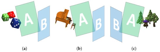
Figure 1.
Wavefield-recording planes for the test scenes Dices, Piano and Woods. Plane B is the image of plane A by a rigid 3D transformation. The wavefield captured in B is the image of the one captured in A by operator . (a) Dices. (b) Piano. (c) Woods.
For Dices and Piano, the transformation between holograms A and B is given by a rotation of around the x axis, a rotation of around the y axis, followed by a shift of 15%, −15% and −50% of the hologram height along the x, y and z axes, respectively. For Woods, the transformation between holograms A and B is given by a rotation of around the x axis, a rotation of around the y axis, followed by a shift of −15%, −15% and −50% of the hologram height along the x, y and z axes respectively.
The tests consisted of comparing the following:
- The ground truth B provided by explicit computation of the tilted hologram in the spatial domain; a CGH algorithm [] is run over the original 3D scene to generate a hologram on the tilted plane.
- The phase space prediction obtained by symplectic transport of the phase space representation of A according to Formula (23).
- The propagated field over tilted plane B based on a frequency domain prediction according to Formula (4), as described in [].
The comparison has been made upon specific numerical reconstructions of the hologram intensity characterized by a focus plane and a pupil. The pupil is a rectangular aperture intended to simulate a viewpoint along the center of the hologram, and the focus plane is chosen so as to accommodate on specific objects of interests in the scene. For the Dices, Piano and Woods scenes, the focus planes have been placed on the red dice, the piano keys and the mushroom house, respectively.
The visual results are shown in Figure 2. The pictures in row (a) are numerical reconstructions of hologram A corresponding to the scenes in the initial poses obtained by computer-generated holography methods.
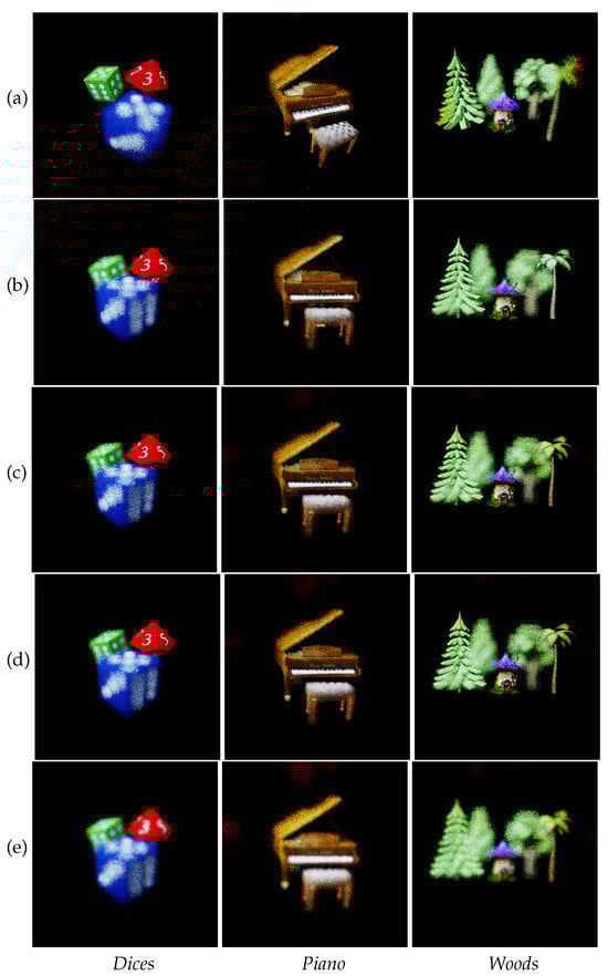
Figure 2.
Numerical reconstructions with focus on specific planes: (a) Hologram A (original pose). (b) Hologram B (target pose). (c) Frequency domain transform of hologram A. (d) Phase space transform of hologram A. (e) Phase space transform of hologram A without phase correction.
Row (b) contains the ground truth of the rotated/translated wavefield. It is the numerical reconstruction of computer-generated hologram B.
The pictures in row (c) are the numerical reconstructions of hologram A transformed by operator in the frequency domain, according to [] and Equation (4).
In row (d), the numerical reconstructions have been computed in phase space using Equation (23). This constitutes the result of our method to be compared to rows (b) and (c).
In row (e), the numerical reconstructions have been computed in phase space using Equation (23), but the corrective phase factor has been voluntarily omitted.
It can be observed by comparing rows (c) and (d) that frequency and phase space computations are almost indistinguishable. Furthermore, by comparing them to the ground truth hologram of row (b), one can see that they both allow us to reproduce the correct perspective.
As mentioned in Section 6, the phase factor of Equation (23) is essential for a correct displacement in phase space; numerical reconstructions of row (e) neglecting this factor show that the new perspective is correct but the focus on the red dice cannot be achieved.
For both frequency and phase space, some unavailable data are missing or toned down according to initial lighting of the scene. For example, on the Dices scene, the eight faces of the red dice is darkened in the target view because it was barely visible in the original one (row (a)). The same can be observed on the piano leg on the right side of the picture.
It is important to note that computing the light propagation in phase space is definitely not a way to achieve better time complexity, but rather, to gain extra functionalities; while the Gabor frame analysis can be performed in less than 1 s, which is approximately the time for computing Equation (4) in the frequency domain, the synthesis of Equation (23) takes around 5 min, even though the partitioning trick mentioned at the beginning of this section allows us to considerably parallelize the processes.
However, while the validity of the phase space approach is measured by its comparison with the frequency domain computation, it is worth stressing again that both approaches are not equivalent: the phase space framework allows us to extract and manipulate semantically meaningful elements of the wavefield that are not directly available in the frequency domain representation. More precisely, the phase space decomposition of the field provides access to the directional information of the ray bundles that can be exploited for advanced editing.
Figure 3 illustrates two examples of such processing, based on a masking described in []; Figure 3a shows a numerical reconstruction of the original Dices hologram A, having a resolution of and pixel pitch of 0.5 m. Figure 3b,c show numerical reconstructions of the partially modified hologram A, in which the green dice has been removed and the blue dice has been first shifted by −512 m, −307.2 m and 204.8 m along the x, y and z axes, respectively, and then rotated by and around the x and y axes, respectively, which would be impossible to realize in the frequency domain.
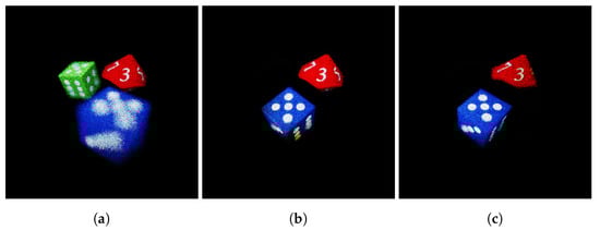
Figure 3.
Hologram editing in phase space. (a) Original hologram (central view). (b,c) Numerical reconstructions of the partially modified hologram A, in which the green dice has been removed and the blue dice has been shifted and rotated (central and bottom–left views, respectively).
These examples illustrate the fact that different parts of the scene may undergo different transformations, which cannot be handled by the frequency domain computation. A typical application of this added functionality could be the motion compensation in hologram video coding [], which was until now constrained to scenes composed of a single object.
8. Conclusions and Perspectives
We have reported a detailed study of tilted propagation expressed in phase space and proposed a method for a computing phase space evolution of classic space–frequency representations of monochromatic fields such as windowed Fourier transforms or Gabor frames.
This method is based on considering the 0-th order of semi-classical expansion of the space–frequency distribution, i.e., the symplectic deformation of the initial distribution. Although it is theoretically only an approximation, the simulations show that the numerical reconstructions are remarkably accurate, both in terms of recovering perspective and focusing on specific planes of the wavefield.
The ability to process coherent light fields in phase space instead of handling integral operators opens the way to many efficient algorithms, especially in digital holography, e.g., for hologram video coding or real-time recomputation of holograms in augmented reality applications.
Although an advantage of phase space is to automatically handle occlusions between the scene objects, 3D transformations are limited by the space region, where the directional information is available, i.e., where it has been recorded by the initial hologram. An interesting extension of the method would be associating it with omnidirectional representations of the scene in order to extend the validity to arbitrary transformations.
Another limitation of the proposed approach, which comes from a limitation of operator itself, is that the rotation discards wave components whose propagation changes from forward to backward. This could be solved by studying the effect of considering as the phase space instead of .
Also, in future work, we plan to extend the study to higher-order terms in order to fully exploit the semiclassical framework, and quantify the error made by using the covariance formula on non-metaplectic operators. Applications to hologram video coding will also be considered.
Author Contributions
Investigation, P.G.; Writing—original draft, P.G.; Writing—review and editing, P.G.; Implementation, A.G. and A.E.R.; Supervision, S.V.N. All authors have read and agreed to the published version of the manuscript.
Funding
This work has been funded by the French government through the National Research Agency (ANR) Investment referenced ANR-A0-AIRT-07.
Institutional Review Board Statement
Not applicable.
Informed Consent Statement
Not applicable.
Data Availability Statement
The data are available on the b-com hologram repository []. The code can be obtained from the corresponding author upon request.
Conflicts of Interest
The authors declare no conflicts of interest.
Appendix A. The Hessian of ϕ Is Non-Degenerate
According to the factorization of Section 5, it is enough to prove it separately when T is a rotation around the x axis with no z propagation and when T is a rotation around the z axis with propagation along the z axis.
Noting , we have in the first case
which is non-zero in all the considered input/output planes’ layouts.
In the second case, we have
Appendix B. Composition of Tilted Propagation Operators
We here prove that the composition of operators of Equation (4) is the operator of the composed underlying rigid transformations. For the sake of conciseness, whenever a dot product involves vectors with mismatching dimensions, the lower dimension vector has to be completed with zeros.
Although the operators are expressed according to a propagation vector along the z axis, they can be generalized to arbitrary shifts in 3D space according to the definition
for a generic vector t and orthogonal transformation U, and .
Since the composition of the two Euclidean transformations and is the transformation , we need to check that . The kernels of and are, respectively,
and
The composition of two such operators has kernel
and hence, as expected. The fact that some frequency variables correspond to backward propagation implies that this equality is only formal, and should be restricted to frequency variables that have been identified as forward propagation according to the criterion of Section 4.
Appendix C. Covariance Formula for the Angular Spectrum
References
- Goodman, J.W. Introduction to Fourier Optics, 3rd ed.; Roberts and Company Publishers: Englewood, CO, USA, 2005. [Google Scholar]
- Matsushima, K. Formulation of the rotational transformation of wave fields and their application to digital holography. Appl. Opt. 2008, 47, D110–D116. [Google Scholar] [CrossRef] [PubMed]
- Muhamad, R.K.; Blinder, D.; Symeonidou, A.; Birnbaum, T.; Watanabe, O.; Schretter, C.; Schelkens, P. Exact global motion compensation for holographic video compression. Appl. Opt. 2019, 58, G204–G217. [Google Scholar] [CrossRef] [PubMed]
- Rhammad, A.E.; Gioia, P.; Gilles, A.; Cagnazzo, M. Progressive hologram transmission using a view-dependent scalable compression scheme. Ann. Des. TéléCommun. 2020, 75, 201–214. [Google Scholar] [CrossRef]
- Birnbaum, T.; Kozacki, T.; Schelkens, P. Providing a Visual Understanding of Holography Through Phase Space Representations. Appl. Sci. 2020, 10, 4766. [Google Scholar] [CrossRef]
- Gröchenig, K. Foundations of Time-Frequency Analysis; Applied and Numerical Harmonic Analysis; Birkhäuser Boston: Boston, MA, USA, 2001. [Google Scholar] [CrossRef]
- Guillemin, V.; Sternberg, S. Semi-Classical Analysis; International Press: Somerville, MA, USA, 2013. [Google Scholar]
- Dragoman, D. Phase Space Correspondence between Classical Optics and Quantum Mechanics. arXiv 2004, arXiv:quantph/0402100v1. [Google Scholar]
- Guillemin, V.; Sternberg, S. Symplectic Techniques in Physics; Cambridge University Press: Cambridge, UK, 1990. [Google Scholar]
- Healy, J.J.; Kutay, M.A.; Ozaktas, H.M.; Sheridan, J.T. (Eds.) Linear Canonical Transforms: Theory and Applications; Number 198 in Springer Series in Optical Sciences; Springer: New York, NY, USA, 2016. [Google Scholar]
- Testorf, M.E.; Hennelly, B.M.; Ojeda-Castañeda, J. Phase-Space Optics: Fundamentals and Applications; McGraw-Hill: New York, NY, USA, 2010. [Google Scholar]
- Gioia, P.; Gilles, A. Method and Device for Coding a Digital Hologram Sequence. Patent WO2021004797A1, 14 January 2021. [Google Scholar]
- Gaim, W.; Lasser, C. Corrections to Wigner type phase space methods. Nonlinearity 2014, 27, 2951–2974. [Google Scholar] [CrossRef][Green Version]
- Berra, M.; Bulai, I.M.; Cordero, E.; Nicola, F. Gabor frames of Gaussian beams for the Schrödinger equation. Appl. Comput. Harmon. Anal. 2017, 43, 94–121. [Google Scholar] [CrossRef]
- Duits, R.; Führ, H.; Janssen, B.; Bruurmijn, M.; Florack, L.; Van Assen, H. Evolution equations on Gabor transforms and their applications. Appl. Comput. Harmon. Anal. 2013, 35, 483–526. [Google Scholar] [CrossRef]
- Wolf, K.B. Geometric Optics on Phase Space; Theoretical and Mathematical Physics; Springer: Berlin/Heidelberg, Germany, 2004. [Google Scholar]
- Zworski, M. Semiclassical Analysis; Graduate Studies in Mathematics; American Mathematical Society: Pawtucket, RI, USA, 2012. [Google Scholar]
- Cordero, E.; Nicola, F.; Rodino, L. Time-Frequency Analysis of Fourier Integral Operators. arXiv 2007, arXiv:0710.3652. [Google Scholar] [CrossRef]
- Gilles, A.; Gioia, P.; Madali, N.; Rhammad, A.E.; Morin, L. Open access dataset of holographic videos for codec analysis and machine learning applications. In Proceedings of the 2023 15th International Conference on Quality of Multimedia Experience (QoMEX), Ghent, Belgium, 20–22 June 2023; pp. 258–263. [Google Scholar] [CrossRef]
- Gilles, A.; Gioia, P.; Cozot, R.; Morin, L. Hybrid approach for fast occlusion processing in computer-generated hologram calculation. Appl. Opt. 2016, 55, 5459–5470. [Google Scholar] [CrossRef] [PubMed]
- Blinder, D.; Schretter, C.; Schelkens, P. Global motion compensation for compressing holographic videos. Opt. Express 2018, 26, 25524–25533. [Google Scholar] [CrossRef] [PubMed]
Disclaimer/Publisher’s Note: The statements, opinions and data contained in all publications are solely those of the individual author(s) and contributor(s) and not of MDPI and/or the editor(s). MDPI and/or the editor(s) disclaim responsibility for any injury to people or property resulting from any ideas, methods, instructions or products referred to in the content. |
© 2024 by the authors. Licensee MDPI, Basel, Switzerland. This article is an open access article distributed under the terms and conditions of the Creative Commons Attribution (CC BY) license (https://creativecommons.org/licenses/by/4.0/).