Vine Copula Modelling of Extreme Temperature, Wind Speed, and Relative Humidity Towards Enhancement of Renewable Energy Production

Abstract

The increasing global reliance on wind and solar energy underscores the critical vulnerability of renewable systems to extreme weather, which can severely disrupt power generation. Accurately modelling the complex, multivariate dependencies of weather extremes is essential for building grid resilience, yet conventional statistical models often fail to capture critical tail dependencies. This study aims to develop a robust framework using vine copulas to model the tail dependencies among key meteorological variables, extreme temperature, wind speed, and relative humidity, across the Eastern Cape province, South Africa, in order to identify optimal seasons for renewable energy production. We first clustered weather stations across the province into five distinct groups using Partitioning Around Medoids (PAM), based on geographical features (elevation, longitude, and latitude). This study explored an automatic selection of the optimal vine copula structure that adequately describes the dependence structure of the meteorological variables employed. The analysis demonstrated that R-vine copulas successfully captured the multivariate tail behaviour of temperature and relative humidity, while D-vine copulas were highly effective for wind speed. The models revealed significant tail dependencies, indicating a high potential for concurrent extreme weather events that impact energy generation. Our findings confirm that vine copulas offer a superior framework for assessing the risks associated with extreme weather to renewable energy systems. The results provide critical insights for regional energy policy and grid resilience planning, highlighting the importance of advanced risk assessment to safeguard renewable energy production against climate extremes.

1. Introduction

1.1. Overview

Renewable energy, such as wind and solar, depends heavily on weather extremes [1]. However, extreme weather severely disrupts renewable energy generation. The growing reliance on wind and solar renewable energy makes weather extremes critical. Extreme weather events disrupt energy supply; hence, accurate modelling of the complex, multivariate dependence structures between and/or across weather variables to enhance renewable energy production is essential [2]. Using fossil fuels to produce energy has been one of the primary causes of climate change [1]. The transition from fossil fuels to renewable energy is necessary for a low-carbon economy, future climate change mitigation, and achieving net-zero emissions through efficiency gains and energy conservation [1,3,4]. Solar and wind energy are abundant and environmentally friendly, as electricity produced by these sources does not emit greenhouse gases into the atmosphere [5,6]. South Africa is among the African countries with abundant renewable energy resources, with the potential to enhance its energy production [7,8,9,10]. However, climate change and the energy crisis in South Africa have sparked concern.

Over 85% of South Africa’s total electricity production comes from coal-fired power stations, with nuclear power plants and renewable sources such as wind, solar, and hydroelectric still accounting for a smaller share of the overall power mix [7,11]. This balance shows the nation’s dependency on coal for power generation [12]. There is a need to increase renewable energy in the energy mix to identify prime locations with greater potential for wind and solar energy production. Integrating renewable energy into the current energy mix can aid in diversifying the national electricity mix, contribute to decarbonisation, and enhance the power supply, among other advantages [12,13].

Natural hazards are becoming more frequent and intense, with spatial implications, necessitating the areal and spatial modelling of the extremes, which is important in environmental statistics [14]. The use of the vine copula to model spatiotemporal dependence among renewable energy outputs across stations, weather variables, or over time has attracted worldwide attention. Various authors have found that vine copula models can capture complex dependencies that traditional bivariate copula models cannot [15,16]. Additionally, studies have employed clustering analyses such as K-means and K-medoids to cluster either stations or seasons, with the number of clusters determined by the maximum silhouette coefficient or the elbow method, among others [17,18]. In the work of [17], latitude and longitude were used to determine the number of clusters of stations using the K-medoids clustering method. Most weather stations are affected by these extreme weather events simultaneously, which also affects renewable energy production [3,9]. Combining clustering analysis with vine copula modelling to capture the tail dependence characteristics of weather variables and to determine the spatiotemporal correlation of renewable energy output is crucial [17]. The present study adopts a seasonal and station-variation approach to model and assess pairwise dependencies among clusters of weather stations and meteorological variables (temperature, relative humidity, and wind speed), identify optimal seasons, and develop a framework to enhance renewable energy production.

1.2. Literature Review

Globally, wind energy is increasingly used to produce electricity [19]. The continuous endeavour to lower carbon emissions in the energy sector depends on renewable energy [1,20]. Nearly two-thirds of the world’s greenhouse gas emissions come from the energy industry [21]. The production of clean energy is highly dependent on weather [21]. According to [22], the top 10 countries utilising mixed renewable energy in terms of capacity are “China, the United States of America (USA), Brazil, India, Germany, Japan, Canada, France, Italy, and Russia”. In 2024, solar energy was expected to surpass all other energy sources globally, making up roughly 40% of renewable energy due to its widespread use in China and India. In 2020, wind and solar power generation grew by 9% and 15%, respectively, with aspirations of achieving at least 32% renewable energy by 2030 [4]. The USA and China have the largest installed capacities of solar photovoltaic systems, among others [23].

Renewable energy sources such as photovoltaic, wind, and hydropower have attracted attention in the literature due to their low pollution and abundant resources [24]. However, renewable energy production is influenced by climate extremes and seasons [18]. Various studies have examined the spatiotemporal correlation of renewable energy output using copula theory, with some authors combining clustering with vine copula models.

A high-dimensional uncertainty scenario generation method based on clustering partitioning was proposed by [17] to model the complex spatiotemporal correlations across multiple wind and solar power plant output scenarios. The cross-validation method was used to determine an optimal number of clusters for K-medoids for multiple power stations. The maximum silhouette coefficients for wind and solar power were found to be 3 and 5, respectively, when stations were clustered by latitude and longitude using K-medoids. The suggested method proved more effective at capturing the spatiotemporal correlation in high-dimensional wind–solar energy systems, enabling efficient linking of output values across different time periods. A C-vine copula was proposed based on spatiotemporal variograms to describe spatial dependence across clusters. A spatiotemporal correlation framework for renewable energy processes was proposed by [18] to explore optimal day-ahead scheduling for a multi-energy coupling system comprising hydro, wind, solar, and hydrogen. The elbow approach was used to identify five as the optimal number of clusters, and the K-means clustering technique was utilised to cluster each season into three categories: average dry scene, wet scene, and normal scene. The R-vine copula models were considered to model the runoff, wind speed, and solar irradiation. The recommended multi-energy system scheduling provides a more resilient and accurate dispatch plan by accounting for the spatiotemporal correlation of renewable sources and scenario generation.

A hybrid stochastic simulation modelling framework was proposed by [25] to integrate a high-dimensional vine copula framework for hourly wind and solar power outputs with discrete–continuous probability distributions. The results of the wind power output seasonal distribution revealed the most abundant wind resources in winter, with summer and winter following, respectively, and the least in winter. This pattern is mainly explained by the subtropical monsoon environment, which fosters interactions between warm and cool air in spring. The authors indicated that wind energy generally surpasses solar output, while summer sees the highest photovoltaic generation, followed by spring and autumn, and winter marks the lowest output. The enhanced vine copula model improves simulation results in terms of deviations and frequencies and successfully reflects the fluctuation in power output by using a hybrid discrete–continuous distribution function. It greatly reduces computational complexity while maintaining the multi-order temporal dependence of wind and solar electricity generation over 10-h intervals.

A complex dependence structure among wind, solar, and hydro energy time series was explored by [2] to evaluate potential methods for modelling correlation and complementarity, focusing on a Brazilian power station. The study addressed the shortcomings of traditional linear correlations with regard to independent assumptions. The C-vine structure was found to be adequate for modelling the spatial correlation between time series of wind speed, solar irradiation, and hydrology. The results revealed that the proposed framework is capable of simulating scenarios and is more accurate at reproducing the statistical attributes and joint behaviour of past complementarity among the variables. Copula models allow the modelling of complex dependencies that traditional linear correlation models cannot capture. To address the integrity and accuracy issue of the output model of the wind–solar combined power generation system, ref. [26] established a spatiotemporal correlation model of wind and solar output that takes into account correlation based on the dynamic copula function and Markov process theory between wind and solar outputs. The outputs of neighbouring wind farms and solar power plants were found to be spatially and temporally correlated; this association is dynamic and varies with time. The dynamic symmetrised Joe Clayton (SJC) copula function adequately described the spatial correlation of photovoltaic and wind energy, as well as its correlation variation features. The dynamic SJC copula is best suited for modelling photovoltaic and wind energy as it better captures the asymmetric tails of the joint output characteristics of wind and solar electricity. In India, daily precipitation, minimum temperatures, and maximum temperatures for the past and future were modelled using a copula to establish the joint behaviour of climate extremes [27]. Copula-based methods were utilised to analyse the joint probability and spatiotemporal behaviour of climate extremes. The authors generated maps that assisted in boosting climate change resilience. The country was prone to both droughts and floods, and many areas previously less prone to precipitation extremes will eventually become more vulnerable in the future.

The energy sector has attracted considerable attention in the literature, including, among others, the review, quantification, modelling, and forecasting of the asymptotic behaviour of extreme climate disasters, solar irradiance, wind speed, renewable energy, and the enhancement of power grid resilience [6,15,19].

Tavakol et al. [28] analysed the simultaneous occurrence of hot, dry, and windy events in the central United States from 1949 to 2018. The Frank copula was selected based on having the smallest Akaike information criterion (AIC) and Bayesian information criterion (BIC). The results showed that the copula approach suggested a higher risk of hot, dry, and windy events. Zhou and Liu [29] investigated the probability of simultaneous excessive temperature and precipitation on China’s interannual scale, encompassing compound events in both the cold and warm seasons. The analysis results showed that across a large portion of the study area, the occurrence probability of the majority of concurrent models will decline. Despite this, favourable changes were observed in the frequency of compound hot/dry events during the warm season across China’s southwest and northeastern regions.

The average minimum and maximum monthly temperature and rainfall were modelled by [30] using a copula in Bahir Dar, Ethiopia. The AIC and BIC were used to select the best marginal distribution and copula. The Clayton copula was selected as the best fit for minimum temperature and rainfall, whereas the Frank copula was found to be the best fit for maximum temperature and rainfall. The results revealed a positive correlation between the minimum temperature and rainfall, whilst a negative correlation between rainfall and maximum temperature was established. In a study by [31], a Frank copula from the Archimedean family was employed to jointly model rainfall and temperature processes as a bivariate distribution using daily rainfall and daily average temperature data from Balaka district, Malawi. The Kendall tau correlation test indicated that temperature and rainfall are positively correlated. The joint modelling of precipitation and temperature was studied by [32] in Kerman Province, Iran, where a copula was employed. The Frank copula was found to be the best model for the recorded data, whereas the Gaussian copula was selected based on the goodness-of-fit results and was utilised for joint modelling.

Mararakanye et al. [19] employed the EVT and copulas to model extreme wind power forecast errors. The authors used forecast error data from 29 South African wind farms, which were classified into two clusters. The study outcomes revealed that the generalised Pareto distribution performed better than the commonly used distributions. Furthermore, significant seasonal and diurnal components of extreme forecast errors were found to depend on the location of the wind farm. The t-student copula was used, and it was found to be essential in providing a regional view of extreme errors. Sigauke and Ravele [33] applied copula models to predict the probability of the simultaneous occurrence of compound extremes in the Limpopo Lowveld Region of South Africa. In the study, elevations were used to classify the temperature and rainfall data into three clusters. The results of the study, when compared with the logistic regression model using the Southern Oscillation Index, revealed changes in the probability of mild, moderate, and severe drought across elevation ranges.

Dependence structure and vine copula studies have been conducted using weather variables by several authors. In a study by [34], a vine copula was applied to establish the dependence structure of the joint distribution between rainfall intensity, wind direction, and wind speed in Qatar. When comparing the observed against the modelled cumulative probabilities using the normalised observations, the trivariate distribution of rainfall intensity, wind direction, and wind speed showed a root mean square error of 0.0072. A copula was used by [35] to analyse and model the dependence structure of wind and solar irradiance across various locations in Germany. The authors also analysed the total energy load and energy exchange of the neighbouring countries. Pair-copula constructions were used to model the high-dimensional joint probability distribution. The authors suggested that wind speeds, solar irradiance, electrical load, and energy import/export are the major uncertain factors that will affect the future energy system. A canonical (C)-vine copula model with 190 dimensions was able to represent the dependencies. Alidoost et al. [36] applied copula-based joint behaviour analyses to assess the impact of climate extreme indices on the price of potatoes and their yield and production. The authors used the C-vine structure to model the complex dependencies. The maximum likelihood estimation (MLE) approach was used to estimate the copula parameters, and the AIC was used to select the best-fitting families within the C-vine structure. Furthermore, the authors also discovered that the copula adequately describes the multivariate dependencies of climate extremes.

Otero et al. [37] conducted a study to analyse copula-based renewable energy droughts across Europe. Energy droughts are referred to as “the periods of low renewable energy production (wind plus solar generation or high residual load)”. The authors suggested that the primary issues impeding the electricity grid are low renewable generation and excessive demand. According to the findings of the joint return periods, moderate winter energy droughts with low renewable production and high residual load tend to occur every six months in European countries, whereas summer events typically occur every 2.4 to 3.6 years. Only a few European nations frequently experience energy shortages, yet summertime unpredictability continues to rise across the continent. To mitigate the impact of load shedding, ref. [10] recommended a techno-economic optimisation of a hybrid renewable energy system that comprised wind turbines, a solar array, a standby diesel engine, and an energy storage unit. Hourly resolution data for wind speed, ambient temperature, and solar radiation for the period 2019 to 2020 were used to carry out the simulations. The authors suggested that an optimised hybrid renewable energy system could alleviate the energy crisis faced by several developing nations.

The present study adopts a clustering approach to classify weather stations based on elevation, latitude, and longitude. Furthermore, the vine copula will be used to capture the dependence structures of weather variables, temperature, wind speed, and relative humidity, among weather stations across the four seasons.

1.3. Contribution and Research Highlights

1.3.1. Contribution

The literature indicates that South Africa has the potential to enhance energy production through its abundant renewable energy resources. A gap exists in the literature regarding the combination of vine copulas and station clustering to model seasonal meteorological variables in relation to renewable energy generation output in South Africa. This study contributes to the body of knowledge and to the existing literature by presenting a novel framework that combines clustering analysis (using the K-medoids clustering method) with R-vine and D-vine models to capture the tail dependence characteristics of meteorological variables (wind speed, relative humidity, and temperature), categorised by seasons (summer, autumn, winter, and spring), across clusters in the Eastern Cape Province of South Africa. By adopting a seasonal and station-variation approach for 32 stations, we enable a systematic and comparable assessment of renewable energy potential, which is a significant enhancement over modelling each station separately.

1.3.2. Research Highlights and Key Findings

The research highlights and key findings of the present study are as follows:

• Using elevation, latitude, and longitude, this study identified five distinct, meaningful clusters of weather stations via the K-medoids technique, confirming the data’s strong suitability for clustering with a Hopkins statistic of 0.67.
• The analysis revealed distinct multivariate tail behaviours for each weather variable; temperature exhibited the strongest and most complex dependence, relative humidity showed weaker and more symmetric dependence, and wind speed displayed unique upper-tail dependence patterns.
• The vine copula models demonstrated strong statistical adequacy. They were found to be highly effective and flexible tools for characterising the non-linear, tail-dependent relationships inherent in multivariate climate data.
• The strong dependency between climate variables identifies the Eastern Cape as a prime location for enhancing renewable energy production. The results provide crucial insights for grid resilience strategies and risk assessment of compound extreme weather events, which are vital for policymakers.

The rest of this paper is organised as follows: Section 2 presents the study area and data source. The methods are described in Section 3, the results and discussions are presented and discussed in Section 4, and Section 5 concludes.

2. Study Area and Data Source

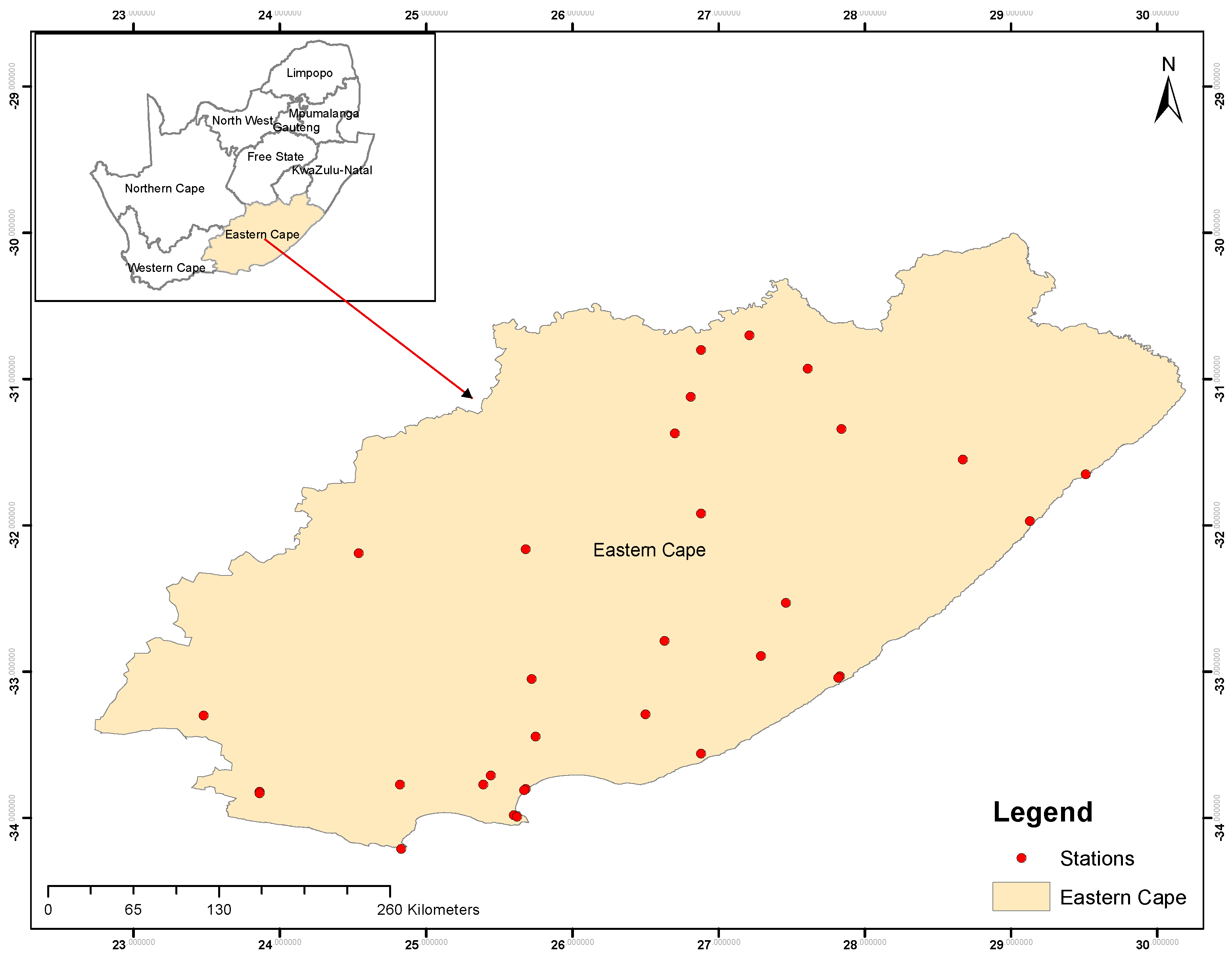
The study area is South Africa’s Eastern Cape Province, covering latitudes $-30$ to $-35$ and longitudes 20 to 30 [10]. South Africa is situated at the southern tip of Africa and comprises nine provinces. The second largest province in South Africa is the Eastern Cape province, following the Northern Cape province. The Eastern Cape province is situated at the southeastern part of South Africa with an area of about 169,000 km² [38]. The neighbouring province to the northwest side is the Northern Cape province and to the west is the Western Cape province [38]. The northern part of the Eastern Cape province includes Lesotho and the Free State province; on the northeastern side is the KwaZulu-Natal province; and on the southern side of the Eastern Cape province is the Indian Ocean. The coastal areas of the Eastern Cape province are characterised by “sub-tropical climatic conditions” [38]. Figure 1 shows the map of South Africa with the nine provinces, the Eastern Cape province, and the spatial distribution of the weather stations in the Eastern Cape province.

This study employs the South African Weather Service and Historical Weather API high-resolution data from Open-Meteo recorded hourly from 1 January 1980 to 31 December 2024. Hourly time series data for climate variables comprising wind speed, humidity, and temperature data for the five clusters, respectively, are used for vine copula modelling. Vine copulas were only fit for one climate variable across five clusters categorised into four seasons: summer (December to February), autumn (March to May), winter (June to August), and spring (September to November). The data is accessible at https://open-meteo.com/en/docs/historical-weather-api (accessed on 10 March 2025). The wind speed data captured by the anemometer was at a height of 10 m, the temperature was recorded in degrees Celsius (°C), and the relative humidity was recorded as a percentage (%).

South Africa has the potential to produce vast amounts of renewable energy. In this study, the extreme temperature, relative humidity, and wind speed data are categorised into four seasons. In South Africa, studies have investigated seasonality and weather station variations in extreme values of weather variables [39,40,41]. Instead of modelling and analysing each station independently, temperature, relative humidity, and wind speed data were categorised into four seasons to highlight seasonal and spatial climate trends and patterns, identify geographical differences, optimise comparability across weather stations, and enhance statistical robustness. Few studies in South Africa have applied seasonal and station variation using a vine copula approach to enhance renewable energy production [6,19].

3. Methods

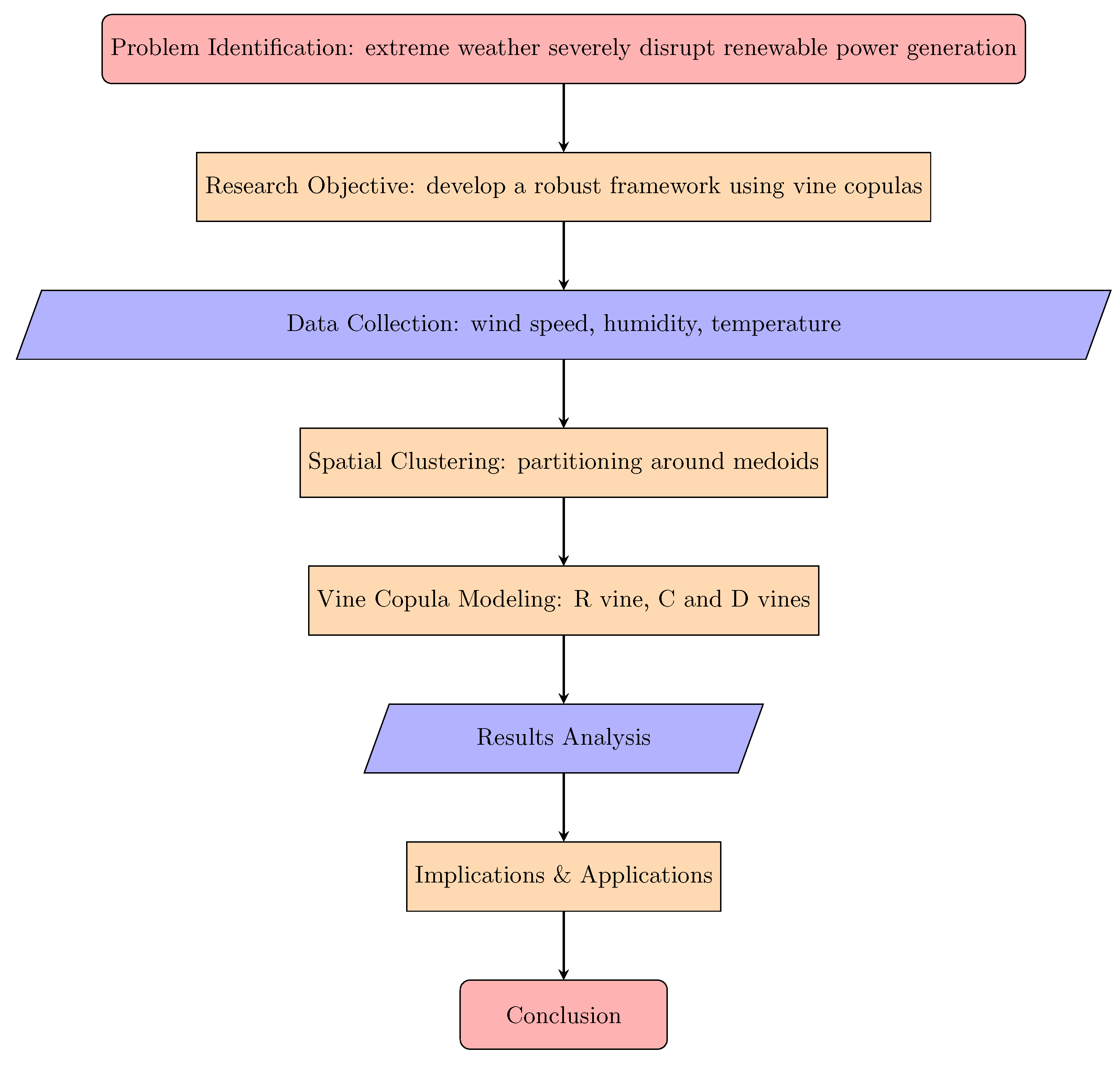
The research methodology flowchart for renewable energy resilience assessment using vine copulas is given in Figure 2. Extreme weather disrupts renewable energy production, which is the problem this study intends to investigate. Based on this problem, this study aims to develop a robust framework using vine copulas to identify the optimal season for renewable energy production. Hourly meteorological time series data are collected from the South African Weather Service, and high-resolution historical weather data from Open-Meteo, recorded from 1 January 1980 to 31 December 2024, are used for vine copula modelling to support the framework development. Spatial clustering of weather stations in the Eastern Cape province of South Africa is used in this study. Vine copula modelling was conducted using R version 4.5.0, with an automatic selection of the suitable vine copula performed using the RVineStructureSelect() function of the VineCopula package in R [42]. The results were analysed, and discussions were conducted to draw conclusions.

3.1. Clustering

3.1.1. Cluster Tendency

The Hopkins statistics proposed by [43] will be used to evaluate the clustering tendency before the clustering techniques and algorithms are applied to this study’s weather station data [44]. Given the weather station data, the Hopkins statistics H is expressed as [45]

$$H={\displaystyle \frac{{\sum }_{i=1}^m{w}_i^d}{{\sum }_{i=1}^m(u_i^d+w_i^d)}},$$

(1)

with the null and alternative hypotheses represented as follows: $H_0$: The weather stations’ data does not contain meaningful clusters; $H_1$: The weather stations’ data contains meaningful clusters [46]. If H is close to 1, it indicates that the null hypothesis is rejected and the station’s data is significantly clusterable [46].

Clustering has been widely used in several studies [45,47,48] to determine the number of clusters prior to applying clustering algorithms. Clustering analysis is an exploratory method that divides the data into smaller groups by identifying groups, or clusters, of items with similar attributes [45,49]. The gap statistic, elbow (WSS), and silhouette methods are employed in this study to identify the optimal number of k clusters for the station’s datasets [47,50].

3.1.2. Gap Statistics

The gap statistic approach uses a standardised null reference distribution to evaluate the comparison between $log\left(W_k\right)$ and its expected value [50,51]. The gap statistic proposed by [45] is expressed as

$${\mathrm{Gap}}_n\left(k\right)=E_n^{*}\left\{log\left(W_k\right)\right\}-log\left(W_k\right),$$

(2)

where $E_n^{*}$ represents the expectation under a sample size n from the reference dataset [50].

3.1.3. Elbow Method

The elbow curve is graphically represented by plotting the within-cluster sum of squares, or the sum of squared error, against the number of clusters [51]. The elbow curve method is denoted by

$$\mathrm{WSS}\left(k\right)=\sum _{i=1}^k\sum _{x_j\in C_i}{\parallel x_j-{\mu }_{C_i}\parallel }^2$$

(3)

where k denotes the number of clusters, $C_i$ denotes the ith cluster, and $\parallel x-{\mu }_i{\parallel }^2$ is the squared Euclidean distance between a data point x and the centroid ${\mu }_i$ [51].

3.1.4. Silhouette Method

The silhouette method uses resolution and cohesion to evaluate cluster quality in a graph, with a range of $-1$ to +1. Data is suitable for clustering if the score is near 1 [48]. In a cluster $S_i$, the silhouette coefficient for the ith dataset member is determined by the association [47]

$$s\left(i\right)={\displaystyle \frac{b\left(i\right)-a\left(i\right)}{max\left\{a\right(i),b(i\left)\right\}}}=\left\{\begin{array}{cc}1-{\displaystyle \frac{a\left(i\right)}{b\left(i\right)}},\hfill & \mathrm{if}a\left(i\right)<b\left(i\right),\hfill \\ 0,\hfill & \mathrm{if}a\left(i\right)=b\left(i\right),\hfill \\ {\displaystyle \frac{b\left(i\right)}{a\left(i\right)}}-1,\hfill & \mathrm{if}a\left(i\right)>b\left(i\right),\hfill \end{array}\right.$$

(4)

where $a_i$ represents the mean intra-cluster distance and $b_i$ represents mean inter-cluster distance [47,48].

3.1.5. Partitioning of Weather Stations

In this study, the K-medoids partitioning method was used to group the 32 weather station data into five clusters. Geospatial variables such as elevation, latitude, and longitude are variables used to cluster the weather stations in the Eastern Cape province, South Africa. An actual centrally located weather station point with the minimum total distance to other weather stations within the cluster is used as the K-medoid. Each of the weather stations with the most similar spatial characteristics was then clustered with the medoids [17,46,52,53].

3.2. Copula Theory

The copula theory was first proposed by Sklar (1959) [54]. Sklar’s theorem is defined as follows.

Theorem 1.

Let G be a d-dimensional distribution function with marginals $F_1,F_2,\dots ,F_n$. Then for all $x_1,x_2,\dots ,x_n\in \mathbb{R}$, there is an n-copula C [6,36,55] expressed as

$$G(x_1,\dots ,x_n)=C(F_1\left(x_1\right),F_2\left(x_2\right),\dots ,F_n\left(x_n\right)),$$

(5)

for some n-dimensional copula C as $C:{[0,1)}^n\to [0,1]$. The multivariate marginal distribution $F_i$ is mapped to the univariate distribution function $f_i$. The multivariate joint density is written as follows [6]:

$$f(x_1,\dots ,x_n)=C(F_1\left(x_1\right),F_2\left(x_2\right),\dots ,F_n\left(x_n\right))\times f_1\left(x_1\right)\times \dots \times f_n\left(x_n\right).$$

(6)

The hourly multivariate time series data of extreme temperature, wind speed, and relative humidity at d-stations are considered in this study. The multivariate copula will be used to model the trivariate dependence of the three climate variables, namely, relative humidity, wind speed, and temperature. For the three random variables X (temperature), Y (wind speed), and R (relative humidity), with the cumulative distribution functions (CDFs) [28] $F_X\left(x\right)=Pr(X\le x),F_Y\left(y\right)=Pr(Y\le y),\mathrm{and}{F}_R\left(r\right)=Pr(R\le r)$, the trivariate joint distribution $\left(C\right)$ is defined as

$$\begin{array}{c}\hfill F(x,y,r)=Pr(X\le x,Y\le y,R\le r)=C(u,v,r),\end{array}$$

(7)

where the three climate extreme variables are less than an established threshold and $u,v,$ and r are the uniformly distributed marginals on $[0,1]$ [28].

3.2.1. Summary of Copula Models

The copula is a multivariate method that allows the marginal distribution of each variable to be individually modelled [56]. There are more than three copula families; the Elliptical copulas, Archimedean copulas, and Extreme Value copulas mentioned in

Table 1. Summary of copula models from [57].

Copula Family	Family	Formulae
Elliptical Copulas	Gaussian Copula	$C_P=\mathsf{\Phi }({\mathsf{\Phi }}^{-1}\left(u_1\right),\dots ,\mathsf{\Phi }\left({\mathsf{\Phi }}^{-1}\left(u_d\right)\right)$
	t-Copula	$C_{v,P}\left(u\right)=t_{v,P}(t_v^{-1}\left(u_1\right),\dots ,t_{v.P}^{-1}{u}_d))$
Archimedean Copulas	Frank Copula	$C_P=\mathsf{\Phi }({\mathsf{\Phi }}^{-1}\left(u_1\right),\dots ,\mathsf{\Phi }\left({\mathsf{\Phi }}^{-1}\left(u_d\right)\right)$
	Gumbel Copula	$C(u,v)=exp\left(-{[{(-\ln u)}^{\theta }+{(-\ln v)}^{\theta }]}^{{\displaystyle \frac{1}{\theta }}}\right)$
	Clayton	$C(u,v)={(u^{-\theta }+v^{-\theta }-1)}^{-{\theta }^{-1}}$
	Joe	$C(u,v)=1-{\left({(1-u)}^{\theta }+{(1-v)}^{\theta }{(1-u)}^{\theta }{(1-v)}^{\theta }\right)}^{{\displaystyle \frac{1}{\theta }}}$
Extreme Value Copulas	Hösler–Reiss	$A\left(t\right)=(1-t)\mathsf{\Phi }\left(z_{1-t}\right)+t\mathsf{\Phi }\left(z_t\right),z_t=({\displaystyle \frac{1}{\lambda }}+{\displaystyle \frac{\lambda }{2}}\ln {\displaystyle \frac{1}{1-t}})$
	Marshall–Olkin	$A\left(t\right)=\max 1-{\alpha }_1(1-t),1-{\alpha }_{2}t$
	t-EV	$A\left(t\right)=(1-t).T_{v+1}\left(z_{1-t}\right)+t.T_{v+1}\left(z_t\right),z_t={(1+v)}^{{\displaystyle \frac{1}{2}}}\left({\left[{\displaystyle \frac{t}{1-t}}\right]}^{{\displaystyle \frac{1}{v}}}-\rho \right){(1-{\rho }^2)}^{{\displaystyle \frac{1}{2}}}$
	Tawn	$A\left(t\right)=(1-{\psi }_1)(1-t)+(1-{\psi }_2)t+{[{\left({\psi }_1(1-t)\right)}^{\theta }+{\left({\psi }_{2}t\right)}^{\theta }]}^{{\displaystyle \frac{1}{\theta }}}$

are the most well-known [28,56]. Table 1 shows the summary of copula models, families, and formulae [50,57].

Much work has been carried out on the three copula families in Table 1 by various authors, including, among others [6,19,20,21,28,30,35,46,50,51].

The bivariate copula models in Table 1 are limited only to pairs of variables. Furthermore, these models fail to capture complex tail dependencies in multivariate weather extremes. The vine copula is more flexible, as it accommodates modelling of three or more variables compared to the bivariate copula families in Table 1. Vine copulas have been explored in South Africa’s financial sector [58,59]. However, there is limited literature on climate extremes and the enhancement of renewable energy production in South Africa. The limited application of vine copulas in renewable energy optimisation inspired the current study to employ vine copulas to develop a vine copula framework for extreme temperature, wind speed, and relative humidity.

3.2.2. Vine Copulas

In accordance with Sklar’s Theorem 1, the corresponding joint distribution function $F(X_1,X_2,\dots ,X_n)$ can be written as

$$F(X_1,X_2,\dots ,X_n)=C_{\theta }(F_1\left(x\right),F_2\left(x\right),\dots ,F_n\left(x\right)),$$

(8)

where $C_{\theta }$ is a copula distribution function and $\theta$ represents an explicit parameter for the function $F_1\left(x\right),F_2\left(x\right),\dots ,F_3\left(x\right)$ to denote the marginal distribution function of random variables [60]. The vine copula is a flexible and advanced technique introduced by [61,62]. The vine copula technique has gained significant interest in various fields, including, among others, water, the environment, and meteorology [60,63,64].

According to [58], “the joint density of a regular vine (R-vine) copula with margins $f_1,\dots ,f_n$ is illustrated by the product of conditional copula densities assigned to the edges of the vine and a product of marginal densities”.

Theorem 2.

Let $(\mathcal{F},\mathcal{V},\mathcal{B})$ be an R-vine copula specification on n-elements. There is a unique distribution F that realises this R-vine copula specification with density [57,64,65]

$$f_{1\dots n}\left(x\right)=\prod _{k=1}^n{f}_k\left(x_k\right)\prod _{i-1}^{n-1}\prod _{e\in E_i}{c}_{Ce,aCe,b;De}(F_{Ce,a|De}\left(x_{Ce,b}\right|{\mathbf{x}}_{De}),F_{Ce,b|De}\left(x_{Ce,b}\right|{\mathit{x}}_{de})),$$

(9)

such that each for each $e\in E_i,i=1,\dots ,d-1$, with $e=\{a,b\}$, we have for the distribution function of $X_{Ce,a}$ and $X_{Ce,b}$, given ${\mathit{X}}_{De}={\mathit{x}}_{De}$ [57],

$$F_{Ce,aCe,b|De}(x_{Ce,a},x_{Ce,b}|{\mathit{x}}_{De})=C_e\left(F_{Ce,a|De}\left(x_{Ce,a}\right|{\mathit{x}}_{De}),F_{Ce,b|De}\left(x_{Ce,b}\right|{\mathit{x}}_{De})\right).$$

Further the one-dimensional margins of F are given by $F_i\left(x_i\right),i=1,\dots ,d$ [57].

The general joint probability density of the R-vine copula is expressed as

$$F(x_1,x_2,\dots ,x_n)=\prod _{k=1}^{n}f\left(x_k\right)\prod _{j=N}^1\prod _{i=n}^{j+1}{C}_{j,i|i+1,\dots ,n}\left\{F\left(x_j\right|x_{i+1},\dots ,x_n),F\left(x_i\right|x_{i+1},\dots ,x_n\right)\},$$

(10)

where j denotes the trees, whereas i runs over the edges in each tree [55].

A study conducted by [55] established that the R-vine copula can be broken down into the canonical vine (C-vine) and drawable vine (D-vine) copulas. The joint probability density of the C-vine copula of dimension n can be written as

$$F(x_1,x_2,\dots ,x_n)=\prod _{k=1}^{n}f\left(x_k\right)\prod _{j=1}^{n-1}\prod _{i=1}^{n-j}{C}_{j,j+1|1,\dots ,j-1}\left\{F\left(x_j\right|x_1,\dots ,x_{j-1}\right),F\left(x_{j+1}\right|x_1,\dots ,x_{j-1}\left)\right\}.$$

(11)

The joint probability density of the D-vine copula is given as

$$F(x_1,x_2,\dots ,x_n)=\prod _{k=1}^{n}f\left(x_k\right)\prod _{j=1}^{n-1}\prod _{i=1}^{n-j}{C}_{i,i+j|i+1,\dots ,i+j-1}\left\{F\left(x_i\right|x_{i+1},\dots ,x_{i+j-1}),F\left(x_{i+j}\right|x_{i+1},\dots ,x_{i+j-1}\right)\},$$

(12)

where j pinpoints the trees, whereas i runs over the edges in each tree [55].

The general joint probability density function for three-dimensional dependence structure [66] can be expressed as

$$\begin{array}{c}\hfill f(x_1,x_2,x_3)=f_1\left(x_1\right).f_2\left(x_2\right).f_3\left(x_3\right).C_{12}\{F_1\left(x_1\right),F_2\left(x_2\right)\}.C_{23}\{F_2\left(x_2\right),F_3\left(x_3\right)\}.\\ \hfill C_{13|2}\{F\left(x_1\right|x_2),F\left(x_3\right|x_2)\},\end{array}$$

(13)

where $x_1$ is extreme temperature, $x_2$ is wind speed, and $x_3$ is the relative humidity [34,55].

The maximum likelihood estimation (MLE) approach will be used for parameter estimation. Results from this study are expected to enhance grid stability and energy policy amid a changing climate.

3.2.3. Dependence Structure

The dependence correlation between two variables can be assessed using Kendall’s tau $\left(\tau \right)$, Spearman’s $(\rho$), and Pearson’s $\left(r\right)$ correlation coefficients. Pearson’s correlation coefficient evaluates the bivariate linear dependence. Both Spearman’s $\left(\rho \right)$ and Kendall’s $\left(\tau \right)$ correlation coefficients are rank-based. Spearman’s $\left(\rho \right)$ estimates the linear and non-linear dependence, whereas Kendall’s tau $\left(\tau \right)$ is a non-parametric rank correlation coefficient used to assess the ordinal dependence among sets of random variables [15]. Kendall’s tau $\left(\tau \right)$ is one of the rank-based dependence measures and therefore invariant with respect to monotonic transformation marginals [57]. Kendall’s tau ranges from −1 to 1, revealing its capability to reach the minimum and maximum values [15]. Kendall’s tau $\left(\tau \right)$ non-parametric rank correlation coefficient will be utilised to evaluate the dependence structure among the meteorological variables, namely temperature, relative humidity, and wind speed.

Let $(x_1,x_2)$ be continuous random variables; then Kendall’s $\tau$ expressed in terms of copula C is given by [67]

$${\tau }_C=4{\int }_0^1{\int }_0^{1}C(u,v)c(u,v)dudv-1,$$

(14)

where ${\tau }_C\in [-1,1]$.

3.2.4. Tail Dependence

Extreme weather events are uncommon in nature, often resulting in significant consequences. Understanding the joint dependence of extremes in the tails is essential. In this study, the pairwise tail dependence will be used to understand the joint dependence of extreme temperature, relative humidity, and wind speed data. Pairwise tail dependence in copulas may be measured using limits for the conditional probabilities $Pr(U_2>u|U_1>u)$ and $Pr(U_2\le u|U_1\le u)$, which may be written as [36]

$$\begin{array}{c}\hfill {\chi }_{up}=\underset{u\to 1}{lim}{\displaystyle \frac{1-2u-C(u,u)}{(1-u)}},{\chi }_{low}=\underset{u\to 0}{lim}{\displaystyle \frac{C(u,u)}{\left(u\right)}},\end{array}$$

(15)

provided these limits exist. If one of these expressions is positive, then there is dependence in the corresponding tail, and otherwise there is independence [36].

3.3. Goodness-of-Fit Tests and Model Selection

3.3.1. Empirical Copula Process

The empirical copula process (ECP) is a goodness-of-fit test for vine copula models using hypothesis tests [68]. The goodness of fit tests

$$H_o:C\in C_o=\{C_O:\theta \in \mathrm{\Theta }\}\mathrm{against}{H}_1:C\in C_o=\{C_O:\theta \notin \mathrm{\Theta }\}$$

(16)

where C indicates the distribution function of the vine copula and $C_0$ is a class of parametric vine copulas, with $\mathrm{\Theta }\subseteq {\mathbb{R}}^p$ being the parameter space of dimension p [68].

The ECP is defined as ${\widehat{C}}_n\left(u\right)-C_{\widehat{{\theta }_n}u}$, with $u=(u_1,\dots ,u_d)\in {[0,1]}^d$; then

$${\widehat{C}}_n\left(u\right)={\displaystyle \frac{1}{n+1}}\sum _{t-1}^n{1}_{\{U_{t1\le u1},\dots ,U_{t1\le ud}\}},$$

(17)

with $C_{\widehat{{\theta }_n}u}$ being the copula with estimated parameter(s) $\widehat{{\theta }_n}$ [68].

3.3.2. Model Selection

Once the marginal distributions are computed, the best-fitting copulas will be selected based on the smallest Akaike information criterion (AIC) and Bayesian information criterion (BIC) [28,34].

According to [57], “for a random copula sample $\mathit{u}$ of size p from an R-vine copula with triple $(\mathcal{V},\mathcal{B}(\mathcal{V}\left)\right),\subseteq \left(\mathcal{B}\right(\mathcal{V}\left)\right)$”, the AIC for the R-vine copula is denoted as

$$\begin{array}{c}\hfill AI{C}_{RV}=-2\sum _{k=1}^n\ln ({\ell }_k(\widehat{\mathit{\theta }}\left(\mathcal{B}\left(\mathcal{V}\right)\right);{\mathit{u}}_k)+2K,\end{array}$$

(18)

and the corresponding BIC is defined as

$$\begin{array}{c}\hfill BI{C}_{RV}=-2\sum _{k=1}^n\ln ({\ell }_k(\widehat{\mathit{\theta }}\left(\mathcal{B}\left(\mathcal{V}\right)\right);{\mathit{u}}_k)+ln\left(n\right)K,\end{array}$$

(19)

where K is the number of model parameters [57].

3.4. Overview of R Package and Data Description

The RVineStructureSelect() function of the VineCopula package in R [42] is utilised to analyse the dependence among extreme temperature, relative humidity, and wind speed across the seasons (summer, autumn, winter, and spring) in the Eastern Cape province of South Africa. The model assesses pairwise dependencies among clusters of weather stations and meteorological variables to identify optimal seasons for enhancing renewable energy production. The RVineStructureSelect() function was used to automatically select the appropriate vine structure and copula pair families for each meteorological variable. The AIC and the BIC were employed for model selection, whereas Kendall’s tau was used to measure the pairwise dependencies. The MLE was used to estimate the parameters of the selected suitable structure and families for the temperature, relative humidity, and wind speed data for the weather stations selected as medoids.

4. Results and Discussions

4.1. Exploratory Data Analysis

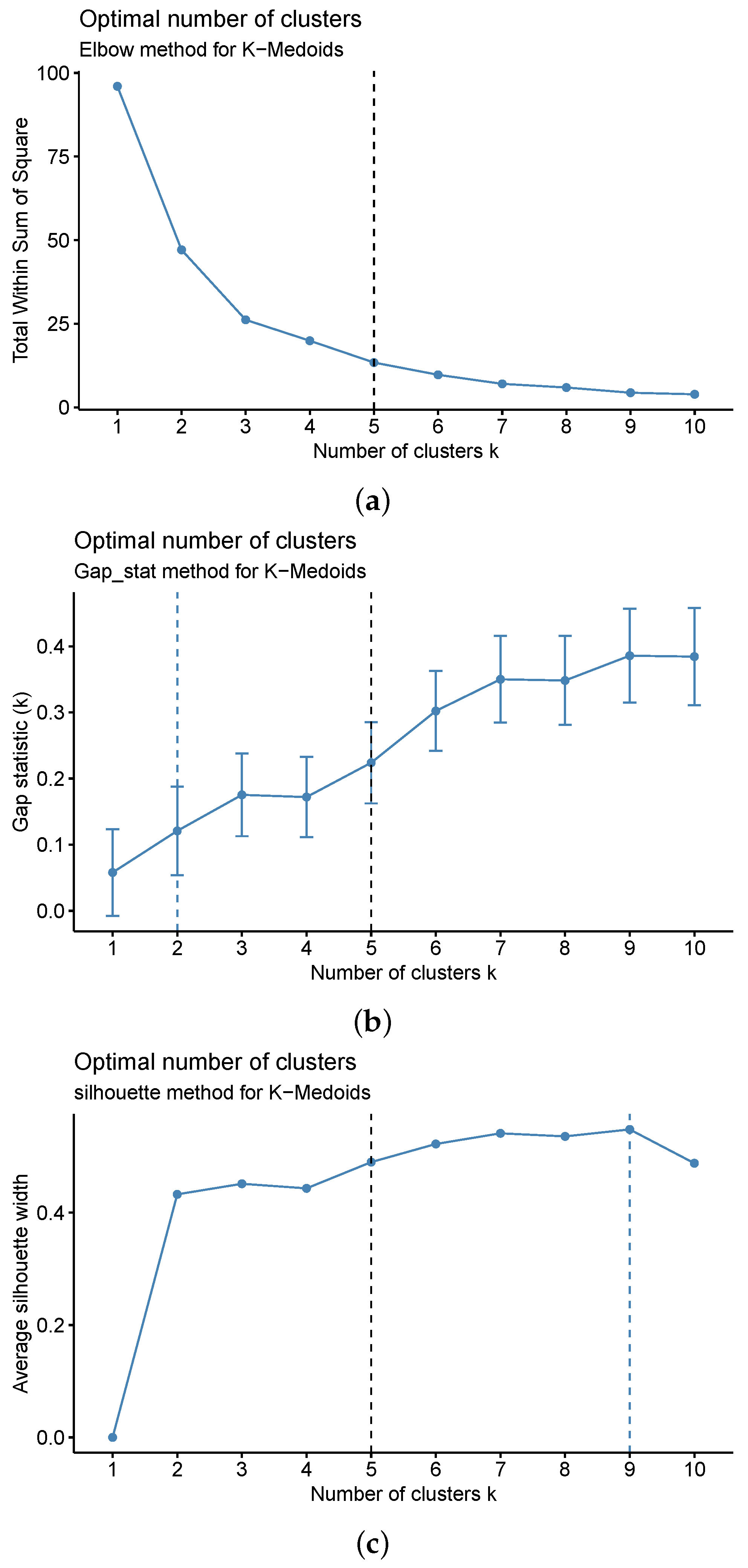
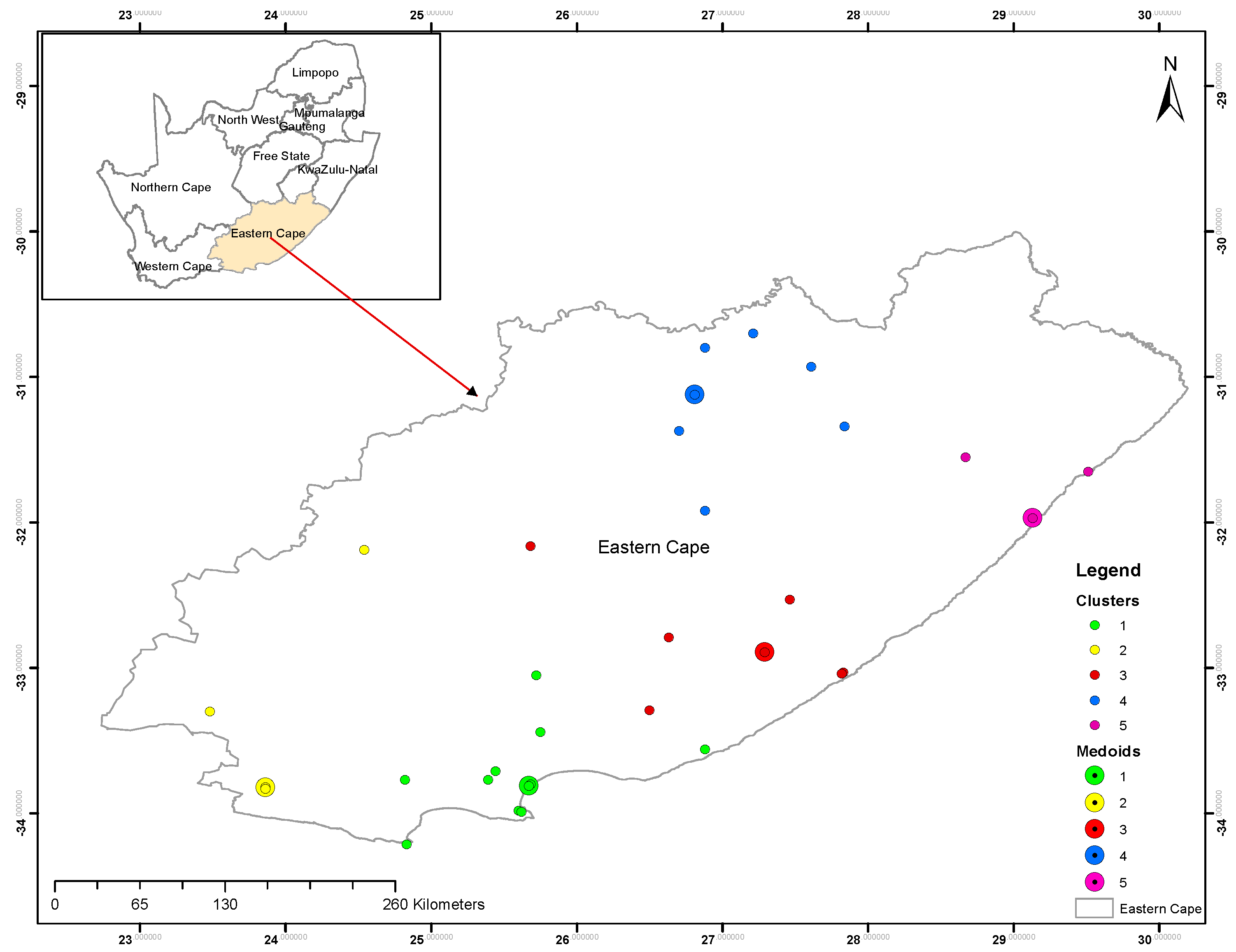
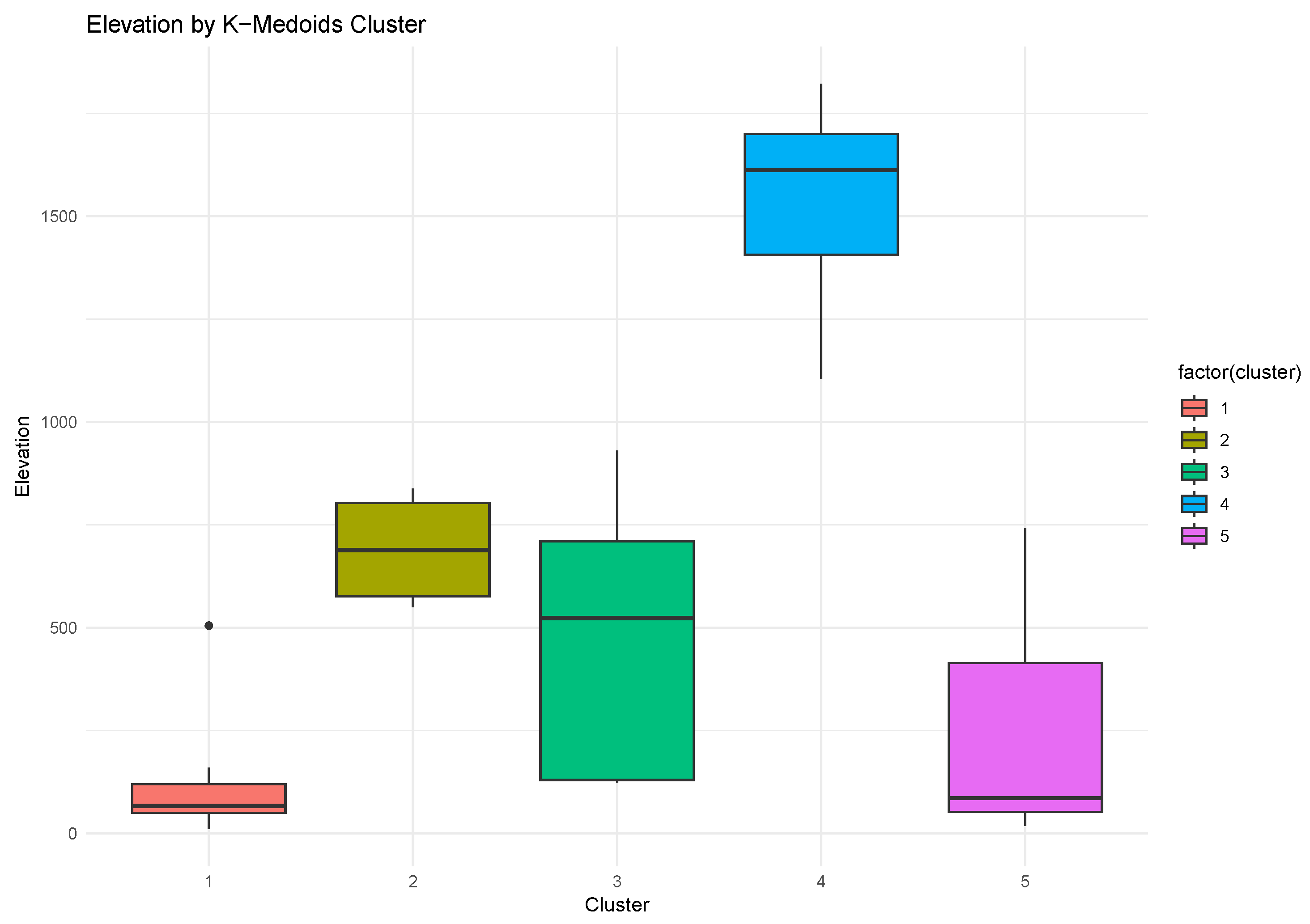
Prior to clustering, the spatial randomness of the weather stations was tested, and the optimal number of clusters was determined using the elbow, gap statistic, and silhouette methods [14,69,70]. Figure 3 show the results of all three methods, suggesting that $k=5$ clusters. The clustering tendency of the weather stations’ data was assessed using the Hopkins statistic. The Hopkins statistic was 0.67, indicating that the weather stations’ data contains meaningful clusters and is well-suited for clustering. Figure 4 and Figure 5 show the spatial distribution in terms of latitude and longitude and the elevations of K-medoids of the five clusters, respectively.

Vine copula models are fitted using seasonal meteorological data, namely temperature, relative humidity, and wind speed, from five stations, which are the medoids of the five clusters. Vine copulas decompose multivariate dependencies into bivariate copulas (pairwise dependencies), allowing for flexible modelling of complex relationships. For each of the five clusters that were obtained, medoids in

Table A1. Names of the Stations of selected K-Mediods.

Station ID	Cluster	Station Name	Latitude	Longitude	Elevation
s14	1	Ngqura Coega	−33.8050	25.6690	50
s2	2	Joubertina School AWS	−33.8240	23.8600	585
s17	3	Bisho	−32.8940	27.2860	593
s26	4	Jamestown	−31.1210	26.8090	1612
s23	5	Coffee Bay	−31.9650	29.1340	87

were used for data analysis. The data was then classified into four seasons, that is, summer (December to February), autumn (March to May), winter (June to August), and spring (September to November), in the Southern Hemisphere.

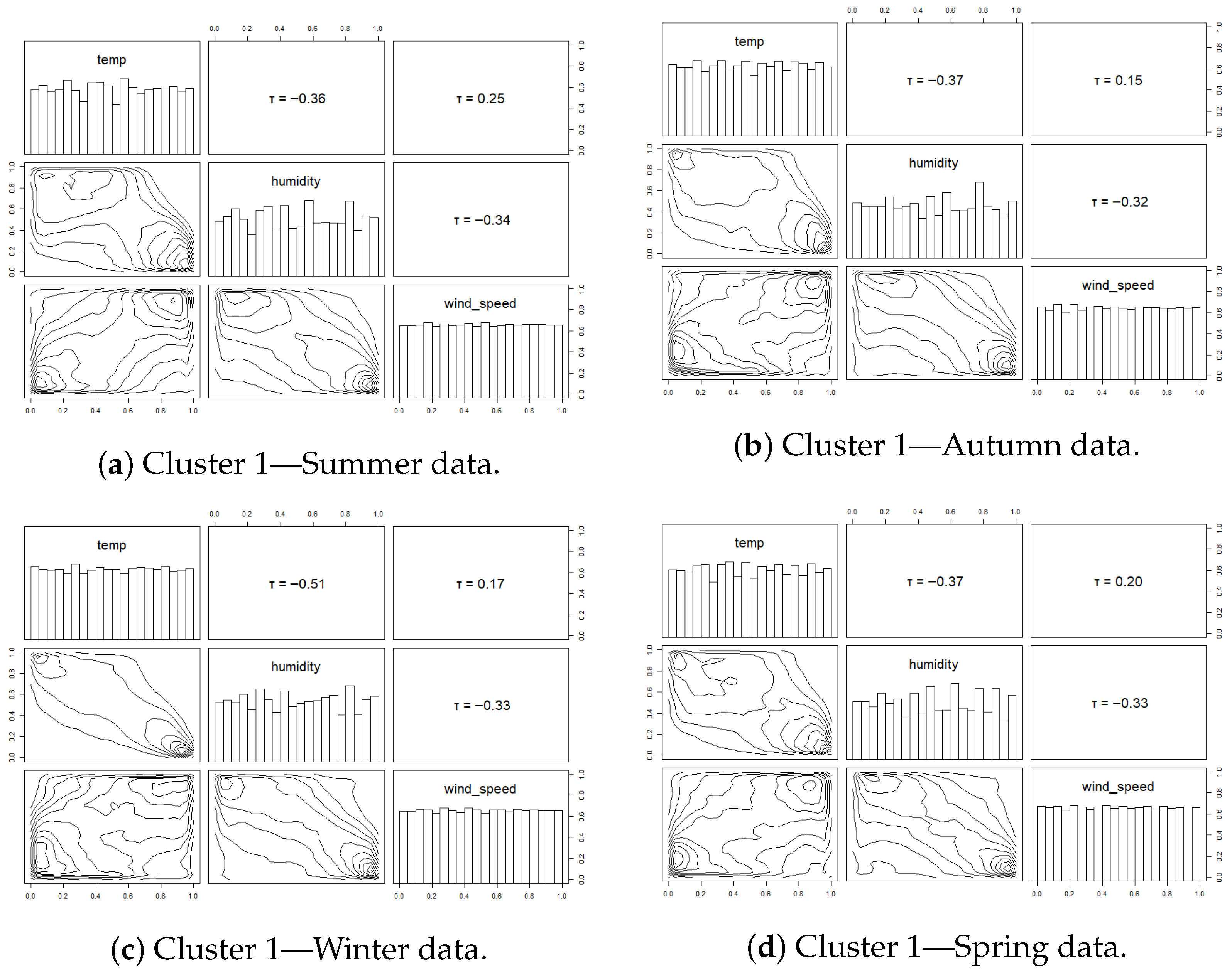
Figure 6 shows the histogram, Kendall’s $\tau$ rank correlation coefficients, and pairwise normalised contour plots for temperature, relative humidity, and wind speed for the four seasons in cluster 1. Based on Kendall’s rank correlation coefficients, temperature and relative humidity tend to be negatively correlated, relative humidity and wind speed are negatively correlated, and there is a very weak positive correlation between temperature and wind speed throughout the four seasons. The exploratory results for clusters 2 to 5 are shown in the Supplementary Materials.

4.2. Summary of the Results

The R-vine was automatically selected for temperature and relative humidity data, whereas the D-vine was automatically selected for wind speed data. Additional findings are available in the Supplementary Materials.

4.2.1. Temperature Dependence Across Seasons

This study analyses temperature dependence across the five medoids in Table A1 using Kendall’s $\tau$, and the R-vine copulas are automatically selected. The results in

Table 2. Kendall’s $\tau$ and copula properties for temperature.

Season	Max $\mathit{\tau }$ (Pair)	Min $\mathit{\tau }$ (Pair)	Dominant Copula (Tree 1)	Tail Dependence
Summer	0.76 (s14–s2)	0.53 (s23–s26)	Student-t	Symmetric
Autumn	0.78 (s14–s2)	0.62 (s2–s23)	Student-t, Gaussian	Symmetric
Winter	0.77 (s14–s2)	0.57 (s14–s26)	Gumbel, Student-t	Asymmetric (Upper)
Spring	0.78 (s14–s2)	0.60 (s26–s2)	Student-t, Survival Gumbel	Symmetric

show that the strongest dependencies were observed in autumn and spring seasons, with Kendall’s $\tau$$\approx 0.75$–$0.78$. The winter season exhibited an asymmetric upper-tail dependence, as captured by the Gumbel copula. The higher trees, that is, trees 2 to 4, exhibited weaker dependencies.

R-Vine Copula Models (Temperature)

In accordance with

Table 3. Key copula families and tail dependence for temperature.

Season	Dominant Copulas (Tree 1)	Tail Dependence	Kendall’s $\mathit{\tau }$ Range	Log-Likelihood
Summer	Student t, Survival Gumbel	Upper tail (0.32–0.49 )	0.58–0.74	312,709.6
Autumn	Student t, Gaussian	Upper tail (0.39–0.50)	0.66–0.76	361,977.8
Winter	Gumbel, Student t	Upper tail (0.43–0.81)	0.63–0.75	316,764.5
Spring	Survival Gumbel, Student t	Upper tail (0.48–0.52)	0.63–0.76	344,956.4

, tree 1 showed upper-tail dependence captured through Gumbel copulas. The tail dependence structure is dominated by the Student-t copulas, with symmetric tail dependence between the temperatures across the seasons. There is a strong tail dependence indicated by Kendall’s $\tau$ ranging from 0.58 to 0.76.

Model Fit Metrics (Temperature)

Table 4. Goodness-of-fit metrics for temperature models.

Season	Log-Likelihood	AIC	BIC
Summer	312,709.6	−625,385	−625,224
Autumn	361,977.8	−723,926	−723,783
Winter	316,764.5	−633,499	−633,357
Spring	344,956.4	−689,879	−689,717

presents the goodness-of-fit metrics for the temperature models. These results indicate that all seasons showed strong model adequacy in capturing the dependence structure among temperature variables across the five stations. The autumn season had the best fit, with the highest log-likelihood of 361,977.8 and the lowest AIC/BIC values of −723,926 and −723,783, respectively, suggesting that autumn is the optimal season for solar renewable energy output.

4.2.2. Relative Humidity Dependence Across Seasons

The Kendall’s $\tau$ correlation matrix was employed to assess the seasonal tail dependence of the five stations, and the R-vine copula has successfully captured the dependencies. Relative humidity showed weaker seasonal dependencies than temperature. According to

Table 5. Kendall’s $\tau$ and copula properties for humidity.

Season	Max $\mathit{\tau }$ (Pair)	Min $\mathit{\tau }$ (Pair)	Dominant Copula (Tree 1)	Tail Dependence
Summer	0.58 (s14–s2)	0.39 (s23–s26)	Frank	Independent
Autumn	0.56 (s14–s17)	0.31 (s23–s26)	Frank, Survival Gumbel	Lower (SG)
Winter	0.60 (s14–s2)	0.30 (s23–s26)	Frank, Student-t	Mixed
Spring	0.59 (s14–s2)	0.32 (s23–s26)	Frank	Independent

, strong dependencies were observed in winter and spring, with $\tau \approx 0.60-0.59$, respectively. The Frank copula dominated in tree 1, indicating a symmetric, tail-independent structure. The relative humidity dependencies were weaker than for temperature, with $\tau \le 0.60$.

R-Vine Copula Models (Relative Humidity)

In accordance with

Table 6. Key copula families and tail dependence for relative humidity.

Season	Dominant Copulas (Tree 1)	Tail Dependence	Kendall’s $\mathit{\tau }$ Range	Log-Likelihood
Summer	Frank	Upper tail (–)	0.51–0.57	170,083.00
Autumn	Frank, Survival Gumbel	Lower tail (0.59–0.60)	0.45–0.52	150,802.40
Winter	Frank, Student t	Upper tail (0.02)	0.38–0.56	151,650.30
Spring	Frank	Upper tail (–)	0.44–0.57	155,965.10

, tree 1 showed lower-tail dependence captured through Survival Gumbel copulas. Tree 1 revealed asymmetric dependence with tail independence.

Model Fit Metrics (Relative Humidity)

Table 7. Goodness-of-fit metrics for humidity models.

Season	Log-Likelihood	AIC	BIC
Summer	170,083.00	−340,138	−340,005
Autumn	150,802.40	−301,585	−301,490
Winter	151,650.30	−303,277	−303,163
Spring	155,965.10	−311,906	−311,792

shows the results of goodness-of-fit metrics for relative humidity models for the four seasons. Summer had a high log-likelihood of 170,083.00, a low AIC of −340,138, and a low BIC of −340,005, indicating a good fit. The results show that summer offers optimal renewable energy output, with stable, regular dependency patterns.

4.2.3. Wind Speed Dependence Across Seasons

The wind speed dependence across the five stations was determined using Kendall’s $\tau$, and the D-vine copulas have captured the dependencies successfully.

Table 8. Summary of Kendall’s tau ranges for wind speed across seasons.

Season	Max $\mathit{\tau }$ (Pair)	Min $\mathit{\tau }$ (Pair)	Dependence Strength
Summer	0.12 (s26–s17)	0.61 (s14–s2)	Weak to moderate
Autumn	0.12 (s26–s17)	0.53 (s14–s2)	Weak to moderate
Winter	0.12 (s26–s23)	0.54 (s14–s2)	Weak to moderate
Spring	0.14 (s17–s26)	0.58 (s14–s2)	Weak to moderate

indicates the summary of Kendall’s $\tau$ ranges for the wind speed across seasons. The strongest dependencies consistently occur between s14 and s2 across all seasons, with Kendall’s $\tau$ ranging from $0.53$ to $0.61$. The weakest dependencies involve s26; for example, for s26–s17 in summer, $\tau =0.12$.

D-Vine Copula Models (Wind Speed)

In accordance with

Table 9. Key copula families and tail dependence for wind speed.

Season	Dominant Copulas (Tree 1)	Tail Dependence	Kendall’s $\mathit{\tau }$ Range	Log-Likelihood
Summer	Gumbel, Survival Clayton	Upper tail (0.18–0.54)	0.17–0.61	99,940.91
Autumn	Gumbel, Survival Clayton	Upper tail (0.26–0.60)	0.21–0.53	88,713.61
Winter	Gumbel, Survival Clayton	Upper tail (0.34–0.61)	0.24–0.55	97,715.73
Spring	Gumbel, Frank	Upper tail (0.23–0.64)	0.19–0.55	102,802.10

, tree 1 showed upper-tail dependence captured through Gumbel/Survival Clayton copulas. The Frank copula appears in spring, suggesting different dependence structures.

Model Fit Metrics (Wind Speed)

Table 10. Goodness-of-fit metrics for wind speed models.

Season	Log-Likelihood	AIC	BIC
Summer	99,940.91	−199,855.8	−199,732.5
Autumn	88,713.61	−177,403.2	−177,289.1
Winter	97,715.73	−195,405.5	−195,281.9
Spring	102,802.10	−205,578.3	−205,454.8

shows the goodness of fit for the wind speed models for the four seasons. Spring had a high log-likelihood of 102,802.10 and a lower AIC and BIC of −205,578.3 and −205,454.8, respectively, showing a good fit. The results show that the optimal season for generating wind power is spring.

4.2.4. Comparative Analysis

Table 11. Comparison of meteorological variable dependencies.

Characteristic	Temperature	Humidity	Wind Speed
Strongest $\tau$ range	0.75–0.78	0.56–0.60	0.53–0.61
Dominant copula	Student-t	Frank	Gumbel/Survival Clayton
Tail dependence	Symmetric/Asymmetric	Mostly independent	Upper tail
Seasonal variation	Moderate	Moderate	Minimal
Model fit (avg LL)	334,102	157,125	97,293

Key: avg LL = average Log-Likelihood.

presents a comparative analysis of the dependencies among the three meteorological variables used in this study, namely temperature, relative humidity, and wind speed. The key findings reveal that temperature shows the strongest dependencies and the most complex tail behaviour. Humidity exhibited the weakest dependencies with mostly symmetric copulas. Wind speed displays intermediate dependence strength but distinctive upper-tail dependence. The pair s14-s2 consistently shows the strongest dependencies across all variables.

5. Conclusions

This study used vine copulas to develop a framework for capturing and modelling the tail dependence of three weather variables, namely temperature, relative humidity, and wind speed, for the five clusters of weather stations in the Eastern Cape province of South Africa. The Hopkins statistic was used to determine the clustering tendency of the weather stations’ data. The Hopkins statistic was 0.67, indicating that the weather stations’ data contains meaningful clusters and is well-suited for clustering. Elevation, latitude, and longitude characteristics were utilised to cluster stations in the Eastern Cape province of South Africa using the K-medoids clustering technique. Five clusters were contained, and the medoids were used for data analysis. The medoids of the five clusters are s14, s2, s17, s26, and s23, respectively, in accordance with Table A1.

The RVineStructureSelect() function of the VineCopula package in R was used to automatically determine a suitable copula pair family and vine structure for each weather variable. The R-vine and D-vine copulas have successfully described the multivariate tail behaviour of the temperature and relative humidity, and the D-vine copulas have successfully described the multivariate tail behaviour of the wind speed variables. Temperature exhibits the strongest and most complex dependence structures. The relative humidity showed a weaker, more symmetric dependence. The wind speed displays distinctive upper-tail dependence patterns. All models demonstrated strong statistical adequacy. Seasonal variations are present, but station pairs (s14–s2) remain consistently strongly correlated. The vine copulas were found to be flexible and adequate for capturing and characterising the dependence structure of multivariate tail behaviour. The vine copulas effectively model non-linear, tail-dependent relationships. Autumn was found to be the optimal season for solar power generation, whereas spring was optimal for wind power generation. However, summer provides the best overall renewable energy generation for both solar and wind power due to consistent, regular dependency patterns influenced by relative humidity.

The strong dependency between the climate variables indicates that the Eastern Cape province is a prime location with the potential to enhance renewable energy production in South Africa. The results will also provide policy engineering insights for grid resilience strategies. Quantifying the risk of compound extremes for renewable energy generation is crucial to policymakers. Future work will evaluate the risk assessment of extreme weather events for the enhancement of renewable energy.

References

1. Russo, M.A.; Carvalho, D.; Martins, N.; Monteiro, A.J.S.E.T. Forecasting the inevitable: A review on the impacts of climate change on renewable energy resources. Sustain. Energy Technol. Assess. 2022, 52, 102283. [Google Scholar] [CrossRef]
2. Iung, A.M.; Cyrino Oliveira, F.L.; Marcato, A.L.; Pereira, G.A. Evaluating the Potential of Copulas for Modeling Correlated Scenarios for Hydro, Wind, and Solar Energy. Forecasting 2025, 7, 7. [Google Scholar] [CrossRef]
3. van der Wiel, K.; Stoop, L.P.; Van Zuijlen, B.R.H.; Blackport, R.; Van den Broek, M.A.; Selten, F.M. Meteorological conditions leading to extreme low variable renewable energy production and extreme high energy shortfall. Renew. Sustain. Energy Rev. 2019, 111, 261–275. [Google Scholar] [CrossRef]
4. Yang, Y.; Javanroodi, K.; Nik, V.M. Climate change and renewable energy generation in Europe—Long-term impact assessment on solar and wind energy using high-resolution future climate data and considering climate uncertainties. Energies 2022, 15, 302. [Google Scholar] [CrossRef]
5. Bakht, M.P.; Salam, Z.; Gul, M.; Anjum, W.; Kamaruddin, M.A.; Khan, N.; Bukar, A.L. The potential role of hybrid renewable energy system for grid intermittency problem: A techno-economic optimisation and comparative analysis. Sustainability 2022, 14, 14045. [Google Scholar] [CrossRef]
6. Sigauke, C.; Ravele, T.; Jhamba, L. Extremal Dependence Modelling of Global Horizontal Irradiance with Temperature and Humidity: An Application Using South African Data. Energies 2022, 15, 5965. [Google Scholar] [CrossRef]
7. Akinbami, O.M.; Oke, S.R.; Bodunrin, M.O. The state of renewable energy development in South Africa: An overview. Alex. Eng. J. 2021, 60, 5077–5093. [Google Scholar] [CrossRef]
8. Ibrahim, I.D.; Hamam, Y.; Alayli, Y.; Jamiru, T.; Sadiku, E.R.; Kupolati, W.K.; Ndambuki, J.M.; Eze, A.A. A review on Africa energy supply through renewable energy production: Nigeria, Cameroon, Ghana and South Africa as a case study. Energy Strategy Rev. 2021, 38, 100740. [Google Scholar] [CrossRef]
9. Apeh, O.O.; Nwulu, N.I. Unlocking economic growth: Harnessing renewable energy to mitigate load shedding in Southern Africa. e-Prime-Adv. Electr. Eng. Electron. Energy 2024, 10, 100869. [Google Scholar] [CrossRef]
10. Landwehr, G.; Lennard, C.; Engelbrecht, F. Wind energy potential of weather systems affecting South Africa’s Eastern Cape Province. Theor. Appl. Climatol. 2024, 15, 3581–3597. [Google Scholar] [CrossRef]
11. De Groot, R.A.F.; Van der Veen, V.G.; Sebitosi, A.B. Comparing solar PV (photovoltaic) with coal-fired electricity production in the centralized network of South Africa. Energy 2013, 55, 823–837. [Google Scholar] [CrossRef]
12. Moulla, D.K.; Attipoe, D.; Mnkandla, E.; Abran, A. Predictive model of energy consumption using machine learning: A case study of residential buildings in South Africa. Sustainability 2024, 16, 4365. [Google Scholar] [CrossRef]
13. Pegels, A. Renewable energy in South Africa: Potentials, barriers and options for support. Energy Policy 2010, 38, 4945–4954. [Google Scholar] [CrossRef]
14. Davison, A.C.; Padoan, S.A.; Ribatet, M. Statistical modeling of spatial extremes. Stat. Sci. 2012, 27, 161–186. [Google Scholar] [CrossRef]
15. Iung, A.M.; Cyrino Oliveira, F.L.; Marcato, A.L.M. A review on modeling variable renewable energy: Complementarity and spatial–temporal dependence. Energies 2023, 16, 1013. [Google Scholar] [CrossRef]
16. Palacios-Rodriguez, F.; Bernardino, E.D.; Mailhot, M. Smooth copula-based generalized extreme value model and spatial interpolation for extreme rainfall in Central Eastern Canada. Environmetrics 2023, 34, e2795. [Google Scholar] [CrossRef]
17. Tan, J.; Zhang, J.; Liu, H.; Lan, B. A high dimensional uncertain scenario generating method for wind power and photovoltaic considering spatiotemporal correlation. Energy 2025, 340, 139224. [Google Scholar] [CrossRef]
18. Chang, P.; Zhu, Q.; Xiao, Y.; Li, S.; Wu, T.; Li, L.; Li, C. Day-ahead optimal scheduling of hydro-wind-solar-hydrogen multi-energy coupling system considering spatiotemporal correlations of renewable energy processes. Renew. Energy 2025, 256, 124431. [Google Scholar] [CrossRef]
19. Mararakanye, N.; Dalton, A.; Bekker, B. Characterizing wind power forecast error using extreme value theory and copulas. IEEE Access 2022, 10, 58547–58557. [Google Scholar] [CrossRef]
20. Moradian, S.; Gharbia, S.; Iglesias, G.; Olbert, A.I. A copula post-processing method for wind power projections under climate change. Energy Convers. Manag. X 2024, 23, 100660. [Google Scholar] [CrossRef]
21. Tedesco, P.; Lenkoski, A.; Bloomfield, H.C.; Sillmann, J. Gaussian copula modeling of extreme cold and weak-wind events over Europe conditioned on winter weather regimes. Environ. Res. Lett. 2023, 18, 034008. [Google Scholar] [CrossRef]
22. Erero, J.L. Impact of loadshedding in South Africa: A CGE analysis. J. Econ. Polit. Econ. 2023, 10, 78–94. [Google Scholar]
23. Solaun, K.; Cerdá, E. Climate change impacts on renewable energy generation. A review of quantitative projections. Renew. Sustain. Energy Rev. 2019, 116, 109415. [Google Scholar] [CrossRef]
24. Min, H.; He, P.; Li, C.; Yang, L.; Xiao, F. The Temporal and Spatial Characteristics of Wind–Photovoltaic–Hydro Hybrid Power Output Based on a Cloud Model and Copula Function. Energies 2024, 17, 1024. [Google Scholar] [CrossRef]
25. Zhu, L.; Xu, B.; Wang, X.; Yue, H.; Mo, R.; Wang, S.; Zhao, Z.; Lu, P. Stochastic Simulation Framework for Renewable Power Output: Integrating Hybrid Discrete-Continuous Distributions with Vine Copula Function. Renew. Energy 2025, 251, 123444. [Google Scholar] [CrossRef]
26. Wang, Z.; Zhu, H.; Zhang, D.; Goh, H.H.; Dong, Y.; Wu, T. Modelling of wind and photovoltaic power output considering dynamic spatio-temporal correlation. Appl. Energy 2023, 352, 121948. [Google Scholar] [CrossRef]
27. Kumar, N.; Goyal, M.K.; Gupta, A.K.; Jha, S.; Das, J.; Madramootoo, C.A. Joint behaviour of climate extremes across India: Past and future. J. Hydrol. 2021, 597, 126185. [Google Scholar] [CrossRef]
28. Tavakol, A.; Rahmani, V.; Harrington, J., Jr. Probability of compound climate extremes in a changing climate: A copula-based study of hot, dry, and windy events in the central United States. Environ. Res. Lett. 2020, 15, 104058. [Google Scholar] [CrossRef]
29. Zhou, P.; Liu, Z. Likelihood of concurrent climate extremes and variations over China. Environ. Res. Lett. 2018, 13, 094023. [Google Scholar] [CrossRef]
30. Fenta, H.M.; Workie, D.L.; Zikie, D.T. Joint modeling of rainfall and temperature in Bahir Dar, Ethiopia: Application of copula. Front. Appl. Math. Stat. 2023, 8, 1058011. [Google Scholar] [CrossRef]
31. Dzupire, N.C.; Ngare, P.; Odongo, L. A copula based bi-variate model for temperature and rainfall processes. Sci. Afr. 2020, 8, e00365. [Google Scholar] [CrossRef]
32. Mesbahzadeh, T.; Miglietta, M.M.; Mirakbari, M.; Soleimani Sardoo, F.; Abdolhoseini, M. Joint modeling of precipitation and temperature using copula theory for current and future prediction under climate change scenarios in arid lands (Case Study, Kerman Province, Iran). Adv. Meteorol. 2019, 2019, 6848049. [Google Scholar] [CrossRef]
33. Sigauke, C.; Ravele, T. Estimating Concurrent Probabilities of Compound Extremes: An Analysis of Temperature and Rainfall Events in the Limpopo Lowveld Region of South Africa. Atmosphere 2024, 15, 557. [Google Scholar] [CrossRef]
34. Qasem, H.; Joergensen, N.E.; Rahman, A.; Samman, H.A.; Al Malki, S.; Al Ansari, A.S. Vine Copula-Based Multivariate Distribution of Rainfall Intensity, Wind Speed, and Wind Direction for Optimizing Qatari Meteorological Stations. Water 2024, 16, 1257. [Google Scholar] [CrossRef]
35. Kloubert, M.L. Probabilistic load flow approach considering dependencies of wind speed, solar irradiance, electrical load and energy exchange with a joint probability distribution model. Energies 2020, 13, 1727. [Google Scholar] [CrossRef]
36. Alidoost, F.; Su, Z.; Stein, A. Evaluating the effects of climate extremes on crop yield, production and price using multivariate distributions: A new copula application. Weather. Clim. Extrem. 2019, 26, 100227. [Google Scholar] [CrossRef]
37. Otero, N.; Martius, O.; Allen, S.; Bloomfield, H.; Schaefli, B. A copula-based assessment of renewable energy droughts across Europe. Renew. Energy 2022, 201, 667–677. [Google Scholar] [CrossRef]
38. Botai, C.M.; Botai, J.O.; Adeola, A.M.; De Wit, J.P.; Ncongwane, K.P.; Zwane, N.N. Drought risk analysis in the Eastern Cape Province of South Africa: The copula lens. Water 2020, 12, 1938. [Google Scholar] [CrossRef]
39. Van der Walt, A.J.; Fitchett, J.M. Statistical classification of South African seasonal divisions on the basis of daily temperature data. S. Afr. J. Sci. 2020, 116, 1–15. [Google Scholar] [CrossRef]
40. Conradie, W.S.; Wolski, P.; Hewitson, B.C. Spatial heterogeneity in rain-bearing winds, seasonality and rainfall variability in southern Africa’s winter rainfall zone. Adv. Stat. Climatol. Meteorol. Oceanogr. 2022, 8, 31–62. [Google Scholar] [CrossRef]
41. Diriba, T.A.; Debusho, L.K. Seasonal and Station Effects Modelling to Extreme Temperature Data in South Africa. Environ. Model. Assess. 2023, 28, 465–489. [Google Scholar] [CrossRef]
42. Nagler, T.; Schepsmeier, U.; Stoeber, J.; Brechmann, E.; Graeler, B.; Erhardt, T. VineCopula: Statistical Inference of Vine Copulas. R Package Version 2.6.1, 2025. Available online: https://github.com/tnagler/vinecopula (accessed on 27 May 2025).
43. Hopkins, B.; Skellam, J.G. A new method for determining the type of distribution of plant individuals. Ann. Bot. 1954, 18, 213–227. [Google Scholar] [CrossRef]
44. Nemukula, M.M.; Sigauke, C.; Chikoore, H.; Bere, A. Modelling drought risk using bivariate spatial extremes: Application to the Limpopo Lowveld Region of South Africa. Climate 2023, 11, 46. [Google Scholar] [CrossRef]
45. Vantas, K.; Sidiropoulos, E. Intra-storm pattern recognition through fuzzy clustering. Hydrology 2021, 8, 57. [Google Scholar] [CrossRef]
46. Apitzsch, C.; Ryeng, J. Cluster Analysis of Mixed Data Types in Credit Risk: A Study of Clustering Algorithms to Detect Customer Segments. 2020. Available online: https://www.diva-portal.org/smash/get/diva2:1444755/FULLTEXT01.pdf (accessed on 27 May 2025).
47. Janse van Vuuren, C.Y.; Vermeulen, H.J. Clustering of wind resource data for the South African renewable energy development zones. J. Energy S. Afr. 2019, 30, 126–143. [Google Scholar] [CrossRef]
48. Yuan, C.; Yang, H. Research on K-value selection method of K-means clustering algorithm. Multidiscip. Sci. J. 2019, 2, 226–235. [Google Scholar]
49. Rodriguez, M.Z.; Comin, C.H.; Casanova, D.; Bruno, O.M.; Amancio, D.R.; Costa, L.D.F.; Rodrigues, F.A. Clustering algorithms: A comparative approach. PLoS ONE 2019, 14, e0210236. [Google Scholar] [CrossRef] [PubMed]
50. Tibshirani, R.; Walther, G.; Hastie, T. Estimating the number of clusters in a data set via the gap statistic. J. R. Stat. Soc. Ser. B 2001, 63, 411–423. [Google Scholar] [CrossRef]
51. Khan, I.K.; Daud, H.; Zainuddin, N.; Sokkalingam, R. Standardizing reference data in gap statistic for selection optimal number of cluster in K-means algorithm. Alex. Eng. J. 2025, 118, 246–260. [Google Scholar] [CrossRef]
52. Jin, X.; Han, J. K-medoids clustering. In Encyclopedia of Machine Learning and Data Mining; Springer: Boston, MA, USA, 2016; pp. 1–3. [Google Scholar] [CrossRef]
53. Kaur, N.K.; Kaur, U.; Singh, D. K-Medoid clustering algorithm-a review. Int. J. Comput. Appl. Technol. 2014, 1, 42–45. [Google Scholar]
54. Sklar, M. Fonctions de répartition à n dimensions et leurs marges. Ann. l’ISUP 1959, 8, 229–231. [Google Scholar]
55. Aas, K.; Czado, C.; Frigessi, A.; Bakken, H. Pair-copula constructions of multiple dependence. Insur. Math. Econ. 2009, 44, 182–198. [Google Scholar] [CrossRef]
56. Czado, C.; Nagler, T. Vine copula based modeling. Annu. Rev. Stat. Its Appl. 2022, 9, 453–477. [Google Scholar] [CrossRef]
57. Czado, C. Analyzing Dependent Data with Vine Copulas: A Practical Guide with R; Springer International Publishing: Berlin/Heidelberg, Germany, 2019. [Google Scholar] [CrossRef]
58. Muteba Mwamba, J.W.; Mwambi, S.M. Assessing market risk in BRICS and oil markets: An application of Markov switching and vine copula. Int. J. Financ. Stud. 2021, 9, 30. [Google Scholar] [CrossRef]
59. Mudiangombe, B.M.; Muteba Mwamba, J.W. Dynamic asymmetric effect of currency risk pricing of exchange rate on equity markets: A regime-switching based C-vine copulas method. Int. J. Financ. Stud. 2022, 10, 72. [Google Scholar] [CrossRef]
60. Yu, R.; Yang, R.; Zhang, C.; Špoljar, M.; Kuczyńska-Kippen, N.; Sang, G. A vine copula-based modeling for identification of multivariate water pollution risk in an interconnected river system network. Water 2020, 12, 2741. [Google Scholar] [CrossRef]
61. Joe, H. Multivariate extreme-value distributions with applications to environmental data. Can. J. Stat. 1994, 22, 47–64. [Google Scholar] [CrossRef]
62. Joe, H. Families of m-variate distributions with given margins and m (m-1)/2 bivariate dependence parameters. Lect.-Notes-Monogr. Ser. 1996, 28, 120–141. [Google Scholar]
63. Bedford, T.; Cooke, R.M. Probability density decomposition for conditionally dependent random variables modeled by vines. Ann. Math. Artif. Intell. 2001, 32, 245–268. [Google Scholar] [CrossRef]
64. Bedford, T.; Cooke, R.M. Vines—A new graphical model for dependent random variables. Ann. Stat. 2002, 30, 1031–1068. [Google Scholar] [CrossRef]
65. Dissmann, J.; Brechmann, E.C.; Czado, C.; Kurowicka, D. Selecting and estimating regular vine copulae and application to financial returns. Comput. Stat. Data Anal. 2013, 59, 52–69. [Google Scholar] [CrossRef]
66. Kurowicka, D.; Joe, H. (Eds.) Dependence Modeling: Vine Copula Handbook; World Scientific: Singapore, 2010. [Google Scholar] [CrossRef]
67. Nelsen, R.B. An Introduction to Copulas; Springer Series in Statistics; Springer: New York, NY, USA, 2006. [Google Scholar] [CrossRef]
68. Schepsmeier, U. Efficient goodness-of-fit tests in multi-dimensional vine copula models. arXiv 2013, arXiv:1309.5808. [Google Scholar]
69. Reynolds, A.P.; Richards, G.; Rayward-Smith, V.J. The application of k-medoids and pam to the clustering of rules. In International Conference on Intelligent Data Engineering and Automated Learning; Springer: Berlin/Heidelberg, Germany, 2004; pp. 173–178. [Google Scholar] [CrossRef]
70. Duan, H.; Li, Q.; He, L.; Zhang, J.; An, H.; Ali, R.; Vazifedoust, M. Climate classification for major cities in China using cluster analysis. Atmosphere 2024, 15, 741. [Google Scholar] [CrossRef]
Figure 1. Map of South Africa, the Eastern Cape province, and the spatial distribution of the weather stations in the Eastern Cape province (Source: Authors’ own contribution).
Mca 31 00019 g001
Figure 2. Vine copula framework for renewable energy resilience assessment.
Mca 31 00019 g002
Figure 3. Number of k clusters for (a) elbow method, (b) gap statistic, and (c) silhouette method.
Mca 31 00019 g003
Figure 4. Eastern Cape map with the spatial distribution of the K-medoids cluster of the weather stations (Source: Authors’ own contribution).
Mca 31 00019 g004
Figure 5. Elevation by K-medoids cluster.
Mca 31 00019 g005
Figure 6. Cluster 1 seasonal exploratory data, including histogram of pseudo copula data, Kendall’s τ rank correlation coefficients, and pairwise normalised contour plots for temperature, relative humidity, and wind speed for (a) summer, (b) autumn, (c) winter, and (d) spring.
Mca 31 00019 g006