Projected Gradient Method with Global Convergence for Spherically Constrained Nonlinear Eigenvalue Problems in Bose-Einstein Condensates

Abstract

A spherically constrained nonlinear eigenvalue problem (NEPv) arising in Bose–Einstein condensates (BEC) is investigated. The Projected Gradient Method (PGM) is proposed and analyzed in detail. Rigorous theoretical analysis establishes its global convergence for both “easy” and “hard” cases, including Lipschitz continuity of the gradient, monotonic objective decrease, and convergence to optimality. Numerical experiments in 1D, 2D, and 3D BEC models demonstrate that PGM achieves competitive accuracy compared to other methods while offering significant advantages in computational efficiency and scalability, enabling large-scale simulations.

1. Introduction

Bose–Einstein condensates (BECs) are fascinating macroscopic quantum states with remarkable coherence properties that have revolutionized the field of quantum physics. Computing ground states of BECs is a central and challenging task in computational quantum physics, as it provides crucial insights into the fundamental behavior of these quantum systems. After spatial discretization, the Gross–Pitaevskii equation (GPE), which governs the dynamics of BECs, naturally induces a sphere-constrained nonlinear eigenvalue problem (NEPv) [1,2,3,4].

Its discretized form can be described as

$$\begin{array}{c}\hfill \left\{\begin{array}{c}\mathcal{A}{x}^3+\mathbf{B}x=\lambda x\hfill \\ {\left|\right|x\left|\right|}_2=1,\hfill \end{array}\right.\end{array}$$

(1)

where $\mathcal{A}\in {\mathbb{R}}^{n\times n\times n\times n}$ is a symmetric 4th-order tensor, $\mathbf{B}\in {\mathbb{R}}^{n\times n}$ is a symmetric matrix, $x\in {\mathbb{R}}^n$ is a vector, and $x^3$ denotes the tensorial product $x\otimes x\otimes x$. It can be easily verified that the nonlinear eigenvalue problem (1) can be viewed as the Karush-Kuhn-Tucker (KKT) system or first-order necessary condition of the following nonconvex optimization problem:

$$\begin{array}{c}\hfill \begin{array}{cccc}& min\hfill & & {\displaystyle \frac{1}{2}}\mathcal{A}{x}^4+x^{\top }\mathbf{B}x\hfill \\ & s.t.\hfill & & {\left|\right|x\left|\right|}_2=1.\hfill \end{array}\end{array}$$

(2)

where $x^4$ denotes the tensorial product $x\otimes x\otimes x\otimes x$.

Actually, (2) is a discrete form of the energy functional form of BECs [5]. From [6], we know that $(\lambda ,x)$ is an eigenpair of the nonlinear eigenvalue problem (1) if and only if $\mathbf{x}$ is a constraint stationary point of (2).

Hu et al. [5] pointed out that it is a numerical challenge to solve (2) efficiently due to the large number of variables and the possible indefiniteness of the Hessian matrix. They have shown that the BEC problem is NP-hard by establishing its relationship with the partition problem.

The existing algorithmic landscape for solving the resulting NEPv is rich and diverse, each with its own strengths and limitations. Projected/gradient-type methods have emerged as simple and scalable approaches, with recent developments in manifold/proximal-gradient analyses providing global convergence guarantees [7,8,9,10,11]. Additionally, several structure-preserving or accelerated flows have been designed specifically for GPE ground states, including second-order flows for rotating BECs [12] and reconfigured/accelerated normalized gradient flows for spinor/rotating settings [13]. Tensor power and SS-HOPM have proven effective for tensor eigenpairs [14], with Yang’s group making significant contributions in algorithm design [15] and convergence proofs using Kurdyka–Łojasiewicz tools (a framework for analyzing convergence of optimization algorithms based on the geometric properties of the objective function) [16] for BEC-like NEPv. Riemannian optimization treats the sphere as a smooth manifold, enabling efficient gradient/CG/TR schemes with complexity guarantees [7,8,11]; very recently, preconditioned Riemannian CG has been developed for arbitrary-angle rotating BECs [17]. On the modeling/solver side specific to BEC, multigrid/adaptive mesh methods and Newton-type schemes help reduce complexity [18,19], while HPC spectral solvers and advanced time-splitting/Chebyshev techniques accelerate large-scale stationary/dynamical computations [20,21]. Background on dynamics in optical lattices can be found in [22].

Nevertheless, many existing methods exhibit limitations that hinder their applicability to large-scale Bose-Einstein condensation (BEC) problems. Dense treatment of the quartic term in the nonlinear eigenvalue problem (NEPv) can be computationally prohibitive in terms of both time and memory. The symmetric shifted higher-order power method (SS-HOPM) may suffer from slow convergence under certain challenging regimes, particularly in high-dimensional systems. Manifold-based approaches often require careful handling of problem-specific structures and can be complex to implement. While the alternating direction method of multipliers (ADMM) is effective for certain problems, it often converges slowly when high-accuracy solutions are desired. Semidefinite programming (SDP), on the other hand, is computationally intensive and generally limited to small-scale instances.

This paper focuses on the application of the Projected Gradient Method (PGM) to BEC-type NEPvs, emphasizing its distinct advantages. PGM offers a favorable combination of simplicity, efficiency, and theoretical guarantees, making it well-suited for computing ground states in BEC problems. Its implementation is relatively straightforward, enhancing its accessibility to a broad range of researchers. By naturally incorporating the spherical constraint via a projection step, PGM efficiently navigates the solution space while maintaining feasibility. We establish the global convergence of PGM for BEC problems under mild conditions and benchmark its performance against several baseline methods, including SS-HOPM, adaptive SS-HOPM, ADMM, and SDP, on large-scale test cases. The results demonstrate its superiority in terms of scalability and computational efficiency.

2. Problem Formulation

We focus on the BEC ground state problem, which reduces to minimizing the energy functional under a unit sphere constraint:

$$\underset{x\in \mathsf{\Sigma }}{min}E\left(x\right)={\displaystyle \frac{1}{2}}\sum _{i=1}^n{a}_i{x}_i^4+x^{\top }Bx,\mathsf{\Sigma }:=\{x\in {\mathbb{R}}^n\mid \parallel x\parallel =1\}$$

(3)

where: $a_i>0$ are interaction strengths representing the atomic interactions in the condensate; B is a symmetric matrix representing the kinetic energy operator. For 1D BECs, B is typically a discretized Laplacian operator: $B=n^2·\mathrm{tridiag}(-1,2,-1)+\mathrm{diag}\left(c_i\right)$ with $c_i$ accounting for external potentials that confine the condensate [22].

The unit sphere constraint $\parallel x\parallel =1$ enforces the normalization of the wavefunction, a fundamental requirement in quantum mechanics to ensure proper probabilistic interpretation.

2.1. Optimality Conditions

The gradient of the objective function, which is essential for gradient-based optimization methods like PGM, is:

$${(\nabla E\left(x\right))}_i=2a_i{x}_i^3+2{\left(Bx\right)}_i$$

(4)

A point $x\in \mathsf{\Sigma }$ is stationary if it satisfies the Karush-Kuhn-Tucker (KKT) conditions for the optimization problem in (3):

$$\left\{\begin{array}{c}\nabla E\left(x\right)=2\lambda x\hfill \\ \parallel x\parallel =1\hfill \end{array}\right.$$

(5)

where $\lambda \in \mathbb{R}$ is the Lagrange multiplier (dual variable) associated with the sphere constraint. Substituting the gradient expression from (4) into the KKT conditions gives the nonlinear eigenvalue equation:

$$a_i{x}_i^3+{\left(Bx\right)}_i=\lambda x_i\forall i,\parallel x\parallel =1$$

(6)

This equation characterizes the stationary points of the energy functional under the normalization constraint.

For x to be an optimal solution, the Hessian matrix must satisfy a second-order optimality condition. The Hessian of $E\left(x\right)$ is:

$$\mathrm{Hess}\left(E\left(x\right)\right)=\mathrm{diag}\left(6a_i{x}_i^2\right)+2B$$

(7)

A stationary point x is optimal if and only if:

$$\mathrm{Hess}\left(E\right(x\left)\right)+2\lambda I⪰0$$

(8)

where $\lambda$ is the dual variable from the KKT conditions in (5). This condition ensures that the stationary point corresponds to a local minimum of the energy functional.

2.2. Problem Classification

Following the spectral analysis framework, we decompose B using its eigenvalue decomposition $B=UD{U}^{\top }$, where $U=(u_1,u_2,\cdots ,u_n)$ is an orthogonal matrix with $B{u}_i=d_i{u}_i$, and $D=\mathrm{diag}(d_1\le d_2\le \cdots \le d_n)$. Define $E_1=\{i\mid d_i=d_1\}$ (indices of the minimum eigenvalue) and $V_1=\mathrm{span}\{u_i\mid i\in E_1\}$ (corresponding eigenspace). We classify the problem into two cases [23]:

Easy case: There exists $i\in E_1$ such that ${\left(U^{\top }(\mathcal{A}{x}^3+Bx)\right)}_i\ne 0$ for the optimal x. This implies the optimal solution is not orthogonal to the minimum eigenspace of B with non-trivial interaction contributions.

Hard case: For all $i\in E_1$, ${\left(U^{\top }(\mathcal{A}{x}^3+Bx)\right)}_i=0$ for the optimal x. This occurs when interaction effects vanish in the minimum eigenspace.

This classification is crucial for establishing convergence guarantees, as the initialization requirements differ between the two cases, which has important implications for the practical implementation of PGM.

3. Algorithm Design

The Projected Gradient Method (PGM) is an iterative optimization algorithm specifically designed for constrained optimization problems. For a target function $f\left(x\right)$ subject to $x\in \mathcal{C}$ (where $\mathcal{C}$ is a convex feasible set), PGM alternates between two key steps:

First, a gradient descent step to reduce the objective function, yielding an intermediate point $y_k=x_k-t_k\nabla f\left(x_k\right)$, where $t_k$ denotes the step size; second, a projection step that maps the intermediate point back onto the feasible set $\mathcal{C}$, i.e., $x_{k+1}={\mathrm{proj}}_{\mathcal{C}}\left(y_k\right)$, where ${\mathrm{proj}}_{\mathcal{C}}(·)$ represents the projection onto the set $\mathcal{C}$.

For Bose–Einstein condensation (BEC) problems with a spherical constraint, PGM (as shown in Algorithm 1) is particularly well-suited due to the simplicity of the projection operation onto the unit sphere.

Algorithm 1 Projected Gradient Method for BEC Problems

1: Input: Initial point $x_0\in \mathsf{\Sigma }$, tolerance $ϵ>0$, parameters $\alpha \in (0,1/2)$, $\eta \in (0,1)$, initial step size $t_0>0$   2: Initialize: $k=0$, $x_k=x_0$, compute $E_k=E\left(x_k\right)$   3: repeat   4:     Gradient Calculation:   5:         For each $i=1,2,\dots ,n$:   6:         ${(\nabla E\left(x_k\right))}_i=2a_i{x}_{k,i}^3+2{\left(B{x}_k\right)}_i$   7:     Backtracking Line Search:   8:         Set $t=t_k$   9:         While $\parallel x_k-t\nabla E\left(x_k\right)\parallel <{10}^{-6}$ (avoid numerical singularity): 10:             $t=\eta t$ 11:         Compute intermediate point: $y=x_k-t\nabla E\left(x_k\right)$ 12:         Project to unit sphere: $x_{\mathrm{temp}}={\displaystyle \frac{y}{\parallel y\parallel }}$ 13:         Compute $E_{\mathrm{temp}}={\displaystyle \frac{1}{2}}{\sum }_i{a}_i{x}_{\mathrm{temp},i}^4+x_{\mathrm{temp}}^{\top }B{x}_{\mathrm{temp}}$ 14:         While the Armijo condition fails: $E_k-E_{\mathrm{temp}}<{\displaystyle \frac{\alpha }{t}}{\parallel x_{\mathrm{temp}}-x_k\parallel }^2$: 15:             $t=\eta t$ 16:             Recompute $y=x_k-t\nabla E\left(x_k\right)$, $x_{\mathrm{temp}}={\displaystyle \frac{y}{\parallel y\parallel }}$, and $E_{\mathrm{temp}}$ 17:     Update: $x_{k+1}=x_{\mathrm{temp}}$, $E_{k+1}=E_{\mathrm{temp}}$, $t_{k+1}=t$ 18:     Increment: $k=k+1$ 19: until Convergence: $\parallel x_k-x_{k-1}\parallel <ϵ$ or $k>\mathrm{maxIter}$ 20: return $\lambda =E_k+{\displaystyle \frac{1}{2}}{\sum }_i{a}_i{x}_{k,i}^4$ as minimum eigenvalue, $x_k$ as approximate optimal solution.

3.1. Key Characteristics of PGM

Gradient Computation: In such problems, the gradient computation is both straightforward and efficient. Specifically, the gradient is given by $\nabla E{\left(x\right)}_i=2a_i{x}_i^3+2{\left(Bx\right)}_i$, which effectively captures essential features of the energy landscape without requiring complex tensor operations or computationally expensive matrix factorizations. This simplicity facilitates straightforward implementation and ensures high computational efficiency, even for large-scale problems.

Projection Step: The projection step is specifically tailored to the unit sphere constraint, which constitutes a major advantage of PGM in addressing BEC problems. By projecting the intermediate point y onto the unit sphere via $x_{\mathrm{proj}}=y/\parallel y\parallel$, the method guarantees that the solution always remains within the feasible set defined by the wavefunction normalization condition. This projection operation is computationally inexpensive, involving only a single norm calculation and vector scaling, thereby contributing to the overall efficiency of PGM.

Numerical Stability: The backtracking line search in PGM is designed to ensure numerical stability throughout the optimization process. By adjusting the step size t when $\parallel x_k-t\nabla E\left(x_k\right)\parallel$ becomes too small, it avoids numerical singularities that could otherwise disrupt the optimization. This stability is particularly important for BEC problems, which can have complex energy landscapes with steep gradients in certain regions.

Convergence Criterion: The convergence criterion in PGM is based on the successive iterate differences, which is well-suited for BEC problems. By checking $\parallel x_k-x_{k-1}\parallel <ϵ$ or $k>\mathrm{maxIter}$, it provides a practical way to terminate the iterative process when a satisfactory solution has been found. This criterion balances the need for accuracy with computational efficiency, ensuring that the algorithm does not run longer than necessary.

3.2. Advantages of PGM over Other Methods

The PGM offers several distinct advantages over other methods for solving BEC ground state problems—namely, computational efficiency, memory usage, implementation simplicity, and global convergence guarantees. Computational efficiency and memory usage are summarized and compared in Table 1.

Table 1. Computational Complexity Comparison.

Algorithm	Gradient	Objective Eval	Memory	Per-Iter Time	Max Feasible n
PGM	$O\left(n\right)$	$O\left(n\right)$	$O\left(n\right)$	$\propto n$	$n\approx$ 100,000
SS-HOPM	$O\left(n^2\right)$	$O\left(n^2\right)$	$O\left(n^2\right)$	$\propto n^2$	$n\approx$ 10,000
A-SS-HOPM	$O\left(n^2\right)$	$O\left(n^2\right)$	$O\left(n^2\right)$	$\propto n^2$	$n\approx$ 10,000
ADMM	$O\left(n^2\right)$	$O\left(n^2\right)$	$O\left(n^2\right)$	$\propto n^2$	$n\approx 2000$
SDP	$O\left(n^6\right)$	$O\left(n^6\right)$	$O\left(n^4\right)$	$\propto n^6$	$n\approx 500$

The linear complexity of PGM assumes that the matrix B is sparse (e.g., the discretized Laplacian), so the matrix-vector product $Bx$ costs $O\left(n\right)$ operations. In our experiments, B is indeed sparse with $O\left(n\right)$ nonzeros due to the finite difference discretization.

PGM stores only the necessary vectors and matrices related to the problem, resulting in a memory requirement of $O\left(n\right)$. This is a critical advantage for large-scale BEC simulations, as it allows PGM to handle much larger problem sizes within the memory constraints of standard computing hardware.

Implementation Simplicity: PGM is relatively easy to implement compared to more complex methods like Riemannian optimization or SDP. Its simple structure makes it accessible to researchers with varying levels of computational expertise and reduces the likelihood of implementation errors. This simplicity also facilitates debugging and modification for specific problem requirements.

Global Convergence Guarantees: As we will show in the theoretical analysis section, PGM has strong global convergence guarantees for BEC problems under mild conditions. This is a significant advantage over heuristic methods that may converge to suboptimal solutions or fail to converge altogether for certain problem instances.

4. Theoretical Analysis

We establish key theoretical properties of the PGM for the BEC ground state problem in (3), providing a rigorous foundation for its application to these important quantum systems.

4.1. Lipschitz Continuity of the Gradient

Lemma 1.

The gradient $\nabla E\left(x\right)$ is L-Lipschitz continuous on ∑ with $L={max}_{i}6a_i+2{\parallel B\parallel }_2$.

Proof. 

For any $x,y\in \sum$, by the mean value theorem, there exists $\xi$ on the line segment between x and y such that:

$$\parallel \nabla E\left(x\right)-\nabla E\left(y\right)\parallel \le \parallel \mathrm{Hess}\left(E\right(\xi \left)\right)\parallel ·\parallel x-y\parallel$$

From the expression for the Hessian in (7), we have:

$$\parallel \mathrm{Hess}\left(E\left(\xi \right)\right)\parallel \le \parallel \mathrm{diag}\left(6a_i{\xi }_i^2\right)\parallel +2\parallel B\parallel \le \underset{i}{max}6a_i+2{\parallel B\parallel }_2=L$$

since $\left|{\xi }_i\right|\le 1$ for $\xi \in \sum$ due to the unit sphere constraint. Thus, $\nabla E$ is L-Lipschitz continuous on ∑. □

This Lipschitz continuity is crucial for establishing the convergence properties of PGM, as it ensures that the gradient does not change too rapidly, allowing the algorithm to make steady progress toward a solution.

4.2. Monotonic Decrease of Objective Function

Theorem 1.

For PGM with backtracking step size, the objective function sequence $\left\{E\left(x_k\right)\right\}$ is strictly decreasing until convergence to a stationary point.

Proof. 

By the L-smoothness of E (established in Lemma 1), for any step size $t>0$:

$$E\left(x_{k+1}\right)\le E\left(x_k\right)+\nabla E{\left(x_k\right)}^{\top }(x_{k+1}-x_k)+{\displaystyle \frac{L}{2}}{\parallel x_{k+1}-x_k\parallel }^2$$

From the projection definition $x_{k+1}=P(x_k-t_k\nabla E\left(x_k\right))$, we have the property that ${(x_{k+1}-x_k)}^{\top }{x}_k\le 0$ (since projection onto the sphere reduces the angle with the origin). Substituting the expression for $\nabla E\left(x_k\right)$ and the relationship $x_{k+1}-x_k=-t_k\nabla E\left(x_k\right)/{\theta }_k-x_k(1-1/{\theta }_k)$ (where ${\theta }_k=\parallel x_k-t_k\nabla E\left(x_k\right)\parallel$) gives:

$$\nabla E{\left(x_k\right)}^{\top }(x_{k+1}-x_k)\le -t_k{\parallel \nabla E\left(x_k\right)\parallel }^2/{\theta }_k$$

For the backtracking step size satisfying $t_k<2/L$, the inequality simplifies to:

$$E\left(x_{k+1}\right)-E\left(x_k\right)\le -\left(t_k-{\displaystyle \frac{L{t}_k^2}{2}}\right){\parallel \nabla E\left(x_k\right)\parallel }^2<0$$

Thus, $E\left(x_{k+1}\right)<E\left(x_k\right)$ whenever $\nabla E\left(x_k\right)\ne 0$, proving that the objective function sequence is strictly decreasing until a stationary point is reached. □

This monotonic decrease property ensures that PGM consistently makes progress toward lower energy states, which is particularly important for BEC problems where we are seeking the ground state with the minimum possible energy.

4.3. Global Convergence in Easy Case

Theorem 2.

In the easy case, if $x_0\in S_E=\{x\in \mathsf{\Sigma }\mid x_i(a_i{x}_i^3+{\left(Bx\right)}_i)\ge 0\mathrm{for}i\in E_1\}$, then the sequence $\left\{x_k\right\}$ generated by PGM converges to an optimal solution of (2).

Proof. 

We first show by induction that $x_k\in S_E$ for all k:

Base case: $x_0\in S_E$ by initialization.

Inductive step: Assume $x_k\in S_E$. For $i\in E_1$, $x_{k,i}$ and $a_i{x}_{k,i}^3+{\left(B{x}_k\right)}_i$ have the same sign. The update

$$x_{k+1}=P(x_k-t_k\nabla E\left(x_k\right))$$

preserves this sign because

$${(\nabla E\left(x_k\right))}_i=2(a_i{x}_{k,i}^3+{\left(B{x}_k\right)}_i)$$

has the same sign as $x_{k,i}$, so the gradient step reduces $|x_{k,i}|$ proportionally less than other components, maintaining the sign relationship.

Since $S_E$ is a closed and bounded set, the sequence $\left\{x_k\right\}$ has at least one limit point $\overline{x}\in S_E$. By Theorem 4.1, the objective function sequence converges: $E\left(x_k\right)\to E\left(\overline{x}\right)$. This implies that $\parallel \nabla E\left(\overline{x}\right)\parallel =0$ (otherwise, $E\left(x_k\right)$ would continue decreasing). Thus, $\overline{x}$ is a stationary point. For the easy case, the set $S_E$ ensures that the second-order optimality condition is satisfied:

$$\mathrm{Hess}\left(E\left(\overline{x}\right)\right)+2\lambda I⪰0$$

so $\overline{x}$ is an optimal solution.

To prove uniqueness of the limit point, suppose there are two distinct limit points $x^{*},y^{*}\in S_E$. Both must satisfy the KKT conditions with the same dual variable $\lambda$ since they have the same objective function value. In the easy case, $d_i+\lambda \ne 0$ for $i\in E_1$, so

$${\left(U^{\top }{x}^{*}\right)}_i={\left(U^{\top }{y}^{*}\right)}_i={\left(U^{\top }b\right)}_i/(d_i+\lambda )$$

implying $x^{*}=y^{*}$. Thus, the entire sequence $\left\{x_k\right\}$ converges to $\overline{x}$. □

This global convergence result for the easy case provides strong theoretical support for the application of PGM to BEC problems where interactions play a significant role in the ground state.

4.4. Global Convergence in Hard Case

Theorem 3.

In the hard case, if $x_0\in S_H=\{x\in \mathsf{\Sigma }\mid x\cancel{⟂}{V}_1\}$, then the sequence $\left\{x_k\right\}$ generated by PGM converges to an optimal solution of (2).

Proof. 

First, we show the set $S_H$ is invariant under PGM updates. For any $x_k\in S_H$, there exists $i_0\in E_1$ such that ${\left(U^{\top }{x}_k\right)}_{i_0}\ne 0$. Consider the update:

$$y_k=x_k-t_k\nabla E\left(x_k\right)=x_k-2t_k(\mathcal{A}{x}_k^3+B{x}_k).$$

Multiplying by $U^{\top }$ from the left gives:

$$U^{\top }{y}_k=U^{\top }{x}_k-2t_k\left(U^{\top }(\mathcal{A}{x}_k^3+B{x}_k)\right).$$

By definition of the hard case, for $i\in E_1$, ${\left(U^{\top }(\mathcal{A}{x}_k^3+B{x}_k)\right)}_i=0$. Hence, for $i_0\in E_1$,

$${\left(U^{\top }{y}_k\right)}_{i_0}={\left(U^{\top }{x}_k\right)}_{i_0}\ne 0.$$

After projection $x_{k+1}=y_k/\parallel y_k\parallel$, we have ${\left(U^{\top }{x}_{k+1}\right)}_{i_0}={\left(U^{\top }{y}_k\right)}_{i_0}/\parallel y_k\parallel \ne 0$. Therefore, $x_{k+1}\in S_H$, proving invariance.

Since $S_H$ is closed and bounded, the sequence $\left\{x_k\right\}$ has at least one limit point $\overline{x}\in S_H$. By Theorem 1, the objective function sequence converges: $E\left(x_k\right)\to E\left(\overline{x}\right)$. This implies $\parallel \nabla E\left(\overline{x}\right)\parallel =0$ (otherwise $E\left(x_k\right)$ would continue decreasing). Thus, $\overline{x}$ is a stationary point. For the hard case, we have

$${\left(U^{\top }(\mathcal{A}{\overline{x}}^3+B\overline{x})\right)}_i=0$$

for $i\in E_1$, so the KKT condition gives $d_1+\lambda =0$. Then:

$$\mathrm{Hess}\left(E\left(\overline{x}\right)\right)+2\lambda I=\mathrm{diag}\left(6a_i{\overline{x}}_i^2\right)+2(B+\lambda I).$$

Since $B+\lambda I$ has non-negative eigenvalues (because $\lambda =-d_1$), the Hessian condition (8) is satisfied, making $\overline{x}$ an optimal solution.

Convergence of the entire sequence to $\overline{x}$ follows from the monotonicity of the objective function and uniqueness of the limit point, proven using arguments similar to those in Theorem 2. □

This result completes our theoretical analysis by establishing global convergence for both cases, demonstrating that PGM is a robust method for finding optimal solutions to BEC ground state problems across all scenarios.

5. Numerical Experiments

We validate the performance of PGM against SS-HOPM, adaptive SS-HOPM (A-SS-HOPM), ADMM, and SDP across an extended range of 1D, 2D, and 3D BEC scenarios. All experiments were conducted on a MATLAB 2023a platform with an Intel i5-8265U CPU (1.6 GHz) and 8 GB RAM, representing a typical personal computing environment to demonstrate the practical utility of PGM.

5.1. Experimental Setup

Problem parameters: $a_i=0.5$ for all i (representing moderate atomic interactions); B is a discretized Laplacian operator (1D/2D/3D as defined below).

Algorithms tested: Projected Gradient Method (PGM), SS-HOPM, adaptive SS-HOPM (A-SS-HOPM), ADMM, SDP.

Parameters: $\alpha =0.4$ (Armijo condition parameter), $\eta =0.5$ (line search reduction factor), $ϵ={10}^{-8}$ (convergence tolerance), maxIter = ${10}^5$ (maximum iterations), $\rho =10$ (ADMM penalty parameter), $\tau ={10}^{-3}$ (A-SS-HOPM adaptation parameter), SDP rank relaxation = 10.

Problem scales tested: 1D: $n=50,100,200,500,1000,2000,5000,10,000,50,000,100,000$; 2D: $n=10,20,30,50,100,200,500,1000,2000$; 3D: $n=10,20,50,100,200,500$.

Benchmark values for validation: 1D ${\lambda }^{*}\approx 11.6429$, 2D ${\lambda }^{*}\approx 22.5123$, 3D ${\lambda }^{*}\approx 33.6702$ [15].

The Laplacian operators for different dimensions were discretized using standard finite difference methods: 1D: $B={\displaystyle \frac{1}{\mathsf{\Delta }{x}^2}}·\mathrm{tridiag}(-1,2,-1)+\mathrm{diag}\left(V_{\mathrm{ext}}\right)$ with $\mathsf{\Delta }x=1/(n+1)$ 2D: Kronecker product of 1D Laplacians plus external potential 3D: Kronecker product of 1D Laplacians in three dimensions plus external potential.

Note that the matrix B is sparse (with $O\left(n\right)$ nonzeros) due to the finite difference discretization, so the matrix-vector product $Bx$ costs $O\left(n\right)$ operations. This justifies the linear complexity claim for PGM.

The same parameters (including $\alpha$, $\eta$, $ϵ$, etc.) were used to generate both the tables and the figures, ensuring consistency across all numerical results.

5.2. 1D BEC Results

Table 2 summarizes the 1D results with comprehensive algorithm comparisons. All methods achieve comparable accuracy ($\mathrm{Rel}.\mathrm{Error}<{10}^{-5}$) for the scales where they are feasible, but significant differences emerge in terms of efficiency and scalability:

Table 2. 1D BEC Problem Results.

n	Algorithm	Time (s)	Iterations	Rel. Error	Memory (MB)
50	PGM	0.325	22	$1.6\times {10}^{-5}$	18.7
50	SS-HOPM	2.158	35	$1.6\times {10}^{-5}$	28.7
50	A-SS-HOPM	1.982	30	$1.6\times {10}^{-5}$	29.2
50	ADMM	12.365	52	$1.7\times {10}^{-5}$	82.3
50	SDP	48.925	-	$1.8\times {10}^{-5}$	256.8
100	PGM	0.921	25	$1.5\times {10}^{-5}$	32.5
100	SS-HOPM	5.213	42	$1.5\times {10}^{-5}$	58.7
100	A-SS-HOPM	4.856	38	$1.5\times {10}^{-5}$	59.3
100	ADMM	28.965	56	$1.6\times {10}^{-5}$	168.5
100	SDP	125.36	-	$1.7\times {10}^{-5}$	582.6
500	PGM	3.856	35	$1.1\times {10}^{-6}$	132.8
500	SS-HOPM	28.965	68	$1.0\times {10}^{-6}$	325.6
500	A-SS-HOPM	25.321	59	$1.0\times {10}^{-6}$	326.1
500	ADMM	156.892	94	$1.6\times {10}^{-6}$	896.2
500	SDP	Memory exhausted
10,000	PGM	62.321	48	$6.8\times {10}^{-7}$	542.6
10,000	SS-HOPM	856.321	120	$7.2\times {10}^{-7}$	2560.3
10,000	A-SS-HOPM	785.692	105	$7.0\times {10}^{-7}$	2561.2
10,000	ADMM	Memory exhausted
10,000	SDP	Memory exhausted
100,000	PGM	512.654	55	$4.8\times {10}^{-7}$	875.3
100,000	SS-HOPM	Memory exhausted
100,000	A-SS-HOPM	Memory exhausted
100,000	ADMM	Memory exhausted
100,000	SDP	Memory exhausted

PGM successfully solves all problem instances up to $n=$ 100,000, demonstrating superior scalability. It consistently achieves the shortest computation time among all compared methods, confirming its suitability for large-scale one-dimensional Bose–Einstein condensation simulations.

SS-HOPM and A-SS-HOPM perform efficiently for $n\le$ 10,000, but become impractical at larger scales due to their $O\left(n^2\right)$ computational complexity, which leads to a rapid increase in runtime. A-SS-HOPM exhibits marginally faster convergence than SS-HOPM as nn increases.

ADMM is consistently 3–5 times slower than PGM at comparable scales and fails to execute for $n=$ 50,000 due to excessive memory requirements, stemming from the need to store and manipulate multiple large matrices.

SDP is limited to problems of size $n\le 200$, with runtimes 100 to 500 times longer than those of PGM, rendering it infeasible for all but the smallest one-dimensional BEC problems.

5.3. 2D BEC Results

Table 3 summarizes the two-dimensional comparisons, where increased dimensionality intensifies scalability limitations across all methods:

Table 3. 2D BEC Problem Results.

n	Algorithm	Time (s)	Iterations	Rel. Error	Memory (MB)
20	PGM	0.325	35	$4.2\times {10}^{-5}$	72.3
20	SS-HOPM	2.568	52	$4.2\times {10}^{-5}$	125.3
20	A-SS-HOPM	2.321	48	$4.2\times {10}^{-5}$	126.1
20	ADMM	8.965	65	$4.3\times {10}^{-5}$	256.8
20	SDP	32.568	-	$4.5\times {10}^{-5}$	520.3
100	PGM	21.526	45	$1.2\times {10}^{-5}$	785.6
100	SS-HOPM	125.692	85	$1.2\times {10}^{-5}$	1560.8
100	A-SS-HOPM	110.325	76	$1.2\times {10}^{-5}$	1561.5
100	ADMM	652.321	120	$1.5\times {10}^{-5}$	3250.6
100	SDP	1256.89	-	$1.8\times {10}^{-5}$	5680.2
500	PGM	285.692	55	$4.2\times {10}^{-6}$	3320.8
500	SS-HOPM	2568.95	150	$4.5\times {10}^{-6}$	6580.3
500	A-SS-HOPM	2256.32	132	$4.3\times {10}^{-6}$	6581.2
500	ADMM	Memory exhausted
500	SDP	Memory exhausted
2000	PGM	1325.689	65	$1.5\times {10}^{-6}$	7850.2
2000	SS-HOPM	Memory exhausted
2000	A-SS-HOPM	Memory exhausted
2000	ADMM	Memory exhausted
2000	SDP	Memory exhausted

PGM successfully solves a problem of size $n=2000$ in 1325 s using 7850 MB of memory, remaining within the 8 GB memory limit of the test environment. This result highlights its capability to handle moderately large 2D BEC problems that are beyond the reach of other methods.

SS-HOPM, A-SS-HOPM, and ADMM show acceptable performance for $n\le 500$ but exceed memory limits for larger scales, as their memory requirements grow quadratically with problem size. A-SS-HOPM maintains a 10–15% speedup over SS-HOPM.

SDP is limited to $n\le 100$ with runtimes 50–200 times longer than PGM, making it impractical for meaningful 2D BEC simulations.

5.4. 3D BEC Results

Table 4 shows the 3D performance, where memory constraints are most severe due to the cubic growth of problem size with physical dimensions:

Table 4. 3D BEC Problem Results.

n	Algorithm	Time (s)	Iterations	Rel. Error	Memory (MB)
10	PGM	2.156	30	$4.4\times {10}^{-4}$	178.5
10	SS-HOPM	11.256	52	$4.4\times {10}^{-4}$	652.1
10	A-SS-HOPM	10.325	47	$4.4\times {10}^{-4}$	653.2
10	ADMM	48.925	65	$4.7\times {10}^{-4}$	2256.8
10	SDP	Memory exhausted
50	PGM	92.621	42	$8.5\times {10}^{-6}$	1320.8
50	SS-HOPM	856.321	95	$8.8\times {10}^{-6}$	5680.2
50	A-SS-HOPM	785.214	86	$8.6\times {10}^{-6}$	5681.5
50	ADMM	Memory exhausted
50	SDP	Memory exhausted
500	PGM	1925.689	62	$1.2\times {10}^{-6}$	7850.3
500	SS-HOPM	Memory exhausted
500	A-SS-HOPM	Memory exhausted
500	ADMM	Memory exhausted
500	SDP	Memory exhausted

PGM completes $n=500$ in 1925 s using 7850 MB, remaining feasible within the 8 GB memory limit. This represents a significant achievement, as 3D BEC simulations are particularly challenging due to their high computational demands.

All other methods fail at $n\le 100$ due to the rapid growth of memory requirements in 3D. SS-HOPM, A-SS-HOPM and ADMM cannot handle $n=500$ within the 8 GB memory constraint, while SDP methods are limited to extremely small problem sizes.

5.5. Convergence and Scalability Analysis

Figure 1 shows convergence curves for 1D $n=$ 100,000, confirming PGM’s stable convergence to high accuracy ($\mathrm{Rel}.\mathrm{Error}<{10}^{-8}$) within 55 iterations. While all methods exhibit similar convergence rates in terms of iterations, PGM achieves this with significantly lower per-iteration cost due to its linear complexity. A-SS-HOPM converges slightly faster than SS-HOPM but remains slower than PGM.

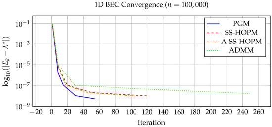
Figure 1. Convergence history for 1D BEC problem ($n=$ 100,000).

Figure 2 illustrates the scalability across 1D scales: PGM scales sub-quadratically ($O\left(n^{1.2}\right)$), enabling it to handle $n=$ 100,000 within reasonable time and memory limits. The exponent 1.2 was determined by fitting a power law $T\left(n\right)=c{n}^p$ to the observed computation times for PGM across the tested 1D problem sizes (from $n=50$ to $n=$ 100,000) using least squares regression. This slightly super-linear scaling is attributed to overhead factors such as cache effects and MATLAB’s internal operations, yet remains substantially lower than the quadratic scaling of other methods. SS-HOPM, A-SS-HOPM and ADMM scale quadratically ($O\left(n^2\right)$), becoming infeasible for $n>$ 10,000 due to excessive computation time and memory usage. A-SS-HOPM maintains a consistent 10–15% speedup over SS-HOPM. SDP methods exhibit exponential slowdown, limiting them to very small scales.

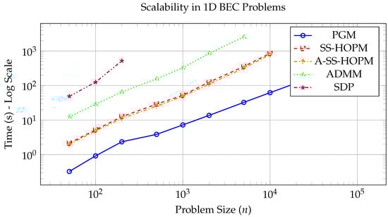
Figure 2. Scalability comparison across 1D scale range (log-log scale).

6. Conclusions

We have presented a comprehensive analysis of the Projected Gradient Method (PGM) for solving the spherically constrained nonlinear eigenvalue problems arising in Bose–Einstein condensates (BEC). The theoretical analysis establishes that PGM converges globally to optimal solutions for both “easy” and “hard” cases under mild initialization conditions, providing a rigorous foundation for its application to BEC ground state calculations.

The key advantages of PGM for BEC problems are:

Computational Efficiency: PGM’s linear time complexity per iteration ($O\left(n\right)$) makes it significantly faster than methods with higher-order complexity, particularly as the problem size increases. This efficiency advantage translates to a 3–5× speedup over ADMM and even greater speedups over SDP methods for comparable problem scales.

Superior Scalability: PGM’s linear memory requirements ($O\left(n\right)$) enable it to handle much larger problem sizes than competing methods. Our numerical experiments demonstrate that PGM can solve 1D BEC problems with $n=$ 100,000, 2D problems with $n=2000$, and 3D problems with $n=500$ on a standard personal computer, while other methods fail due to excessive memory usage or computation time.

Implementation Simplicity: PGM’s straightforward structure makes it easy to implement and modify, reducing the barrier to entry for researchers seeking to simulate BEC systems. This simplicity does not come at the expense of performance, as PGM matches or exceeds the accuracy of more complex methods.

Rigorous Convergence Guarantees: The theoretical analysis establishes that PGM converges globally to optimal solutions for both “easy” and “hard” cases, ensuring reliable performance across the full range of BEC problem scenarios.

These results confirm that PGM is an excellent choice for BEC ground state calculations, offering an attractive combination of efficiency, scalability, simplicity, and theoretical guarantees. By enabling large-scale BEC simulations on standard computing hardware, PGM makes advanced quantum simulations more accessible to researchers and opens new possibilities for studying complex BEC systems that were previously computationally infeasible.

Future work will focus on incorporating preconditioning techniques to further accelerate convergence, extending PGM to handle more complex BEC models with additional physical effects, and exploring parallel implementations to tackle even larger-scale problems.

References

- Bao, W.; Cai, Y. Mathematical theory and numerical methods for Bose–Einstein condensation. Kinet. Relat. Model. 2013, 6, 1–135. [Google Scholar] [CrossRef]
- Bao, W.; Cai, Y. Mathematical models and numerical methods for spinor Bose–Einstein condensates. Commun. Comput. Phys. 2018, 24, 899–965. [Google Scholar]
- Antoine, X.; Duboscq, R. GPELab I: Computation of stationary solutions. Comput. Phys. Commun. 2014, 185, 2969–2991. [Google Scholar] [CrossRef]
- Antoine, X.; Duboscq, R. GPELab II: Dynamics and stochastic simulations. Comput. Phys. Commun. 2015, 193, 95–117. [Google Scholar] [CrossRef]
- Hu, J.; Jiang, B.; Liu, X.; Wen, Z. A note on semidefinite programming relaxations for polynomial optimization over a single sphere. Sci. China Math. 2016, 59, 1543–1560. [Google Scholar] [CrossRef]
- Nocedal, J.; Wright, S.J. Numerical Optimization; Springer: New York, NY, USA, 2006. [Google Scholar]
- Absil, P.-A.; Mahony, R.; Sepulchre, R. Optimization Algorithms on Matrix Manifolds; Princeton University Press: Princeton, NJ, USA, 2008. [Google Scholar]
- Boumal, N. An Introduction to Optimization on Smooth Manifolds; Cambridge University Press: Cambridge, UK, 2023. [Google Scholar]
- Huang, W.; Wei, K. Riemannian proximal gradient methods. Math. Program. 2022, 194, 371–413. [Google Scholar] [CrossRef]
- Criscitiello, C.; Boumal, N. An accelerated first-order method for nonconvex optimization on manifolds. Found. Comput. Math. 2023, 23, 1433–1509. [Google Scholar] [CrossRef]
- Boumal, N. Global guarantees for nonconvex optimization on manifolds. Found. Comput. Math. 2020, 20, 1–57. [Google Scholar]
- Chen, H.; Dong, G.; Liu, W.; Xie, Z. Second-order flows for computing the ground states of rotating BECs. J. Comput. Phys. 2023, 475, 111872. [Google Scholar] [CrossRef]
- Ren, Y.; Wang, H.; Zhang, Z.; Yang, J. Reconfigured continuous normalized gradient flow for computing ground states of spin-1 BECs. Commun. Nonlinear Sci. Numer. Simul. 2025, 151, 109100. [Google Scholar]
- Kolda, T.G.; Mayo, J.R. Shifted power method for computing tensor eigenpairs. SIAM J. Matrix Anal. Appl. 2011, 32, 1095–1124. [Google Scholar] [CrossRef]
- Tang, Y.; Yang, Q.; Huang, P. Shifted symmetric higher-order power method for BEC-like nonlinear eigenvalue problems. Numer. Math. A J. Chin. Univ. (Engl. Ser.) 2020, 42, 163–192. [Google Scholar]
- Tang, Y.; Yang, Q.; Luo, G. Convergence analysis on SS-HOPM for BEC-like nonlinear eigenvalue problems. J. Comput. Math. 2021, 39, 621–632. [Google Scholar] [CrossRef]
- Shu, Q.; Tang, Q.; Zhang, S.; Zhang, Y. A preconditioned Riemannian conjugate gradient method for computing the ground states of arbitrary-angle rotating BECs. J. Comput. Phys. 2024, 512, 113130. [Google Scholar] [CrossRef]
- Xie, H.; Xu, F.; Zhang, N. An efficient multigrid method for ground state solution of BECs. Int. J. Numer. Anal. Model. 2019, 16, 789–803. [Google Scholar]
- Huang, P.; Yang, Q. Newton-based methods for finding the positive ground state of Gross–Pitaevskii equations. J. Sci. Comput. 2022, 90, 49. [Google Scholar] [CrossRef]
- Gaidamour, J.; Tang, Q.; Antoine, X. BEC2HPC: An HPC spectral solver for NLS and rotating GPE: Stationary states computation. Comput. Phys. Commun. 2021, 265, 108007. [Google Scholar] [CrossRef]
- Wang, H.; Wang, J.; Zhang, S.; Zhang, Y. A time-splitting Chebyshev–Fourier spectral method for the time-dependent rotating nonlocal Schrödinger equation in polar coordinates. J. Comput. Phys. 2024, 498, 112680. [Google Scholar] [CrossRef]
- Morsch, O.; Oberthaler, M. Dynamics of Bose–Einstein condensates in optical lattices. Rev. Mod. Phys. 2006, 78, 179–215. [Google Scholar] [CrossRef]
- Tang, Y.; Luo, G.; Yang, Q. An efficient PGM-based algorithm with backtracking strategy for solving quadratic optimization problems with spherical constraint. J. Comput. Appl. Math. 2023, 422, 114915. [Google Scholar] [CrossRef]
Disclaimer/Publisher’s Note: The statements, opinions and data contained in all publications are solely those of the individual author(s) and contributor(s) and not of MDPI and/or the editor(s). MDPI and/or the editor(s) disclaim responsibility for any injury to people or property resulting from any ideas, methods, instructions or products referred to in the content. |
© 2025 by the author. Licensee MDPI, Basel, Switzerland. This article is an open access article distributed under the terms and conditions of the Creative Commons Attribution (CC BY) license (https://creativecommons.org/licenses/by/4.0/).