Fractional Diffusion: A Structured Approach to Application with Examples

Abstract

Time-fractional evolution equations for probability distributions provide a means of representing an important class of stochastic processes. Their solutions have features that are important in modeling anomalous diffusion and a variety of other real-world applications, like the search patterns of predators or queuing problems. However, these equations are usually not included in current physics education, as the underlying mathematics might be considered too advanced. In the following, we present a novel approach to understanding time-fractional diffusion equations and their solutions for practical applications. This approach shifts the focus to the physical rather than the in-depth mathematical properties typically studied for this topic. We introduce the fractional differential operator simply as an identity operation on generalizations of exponential functions. This shifts the emphasis to the actual functions of fractional derivatives instead of what they are. This concept is applied to a discrete one-dimensional time-fractional diffusion equation on a finite interval modeling anomalous subdiffusion. Examples and tasks are provided for readers to allow interactive learning.

1. Introduction

Diffusion can be characterized by the spreading of particles in space due to random movements. One envisions Brownian motion, where particles move and collide, exchanging kinetic energy with each other and their surroundings [1,2]. For this normal Brownian-like diffusion, particles follow random paths over time, gradually increasing their mean square displacement (MSD), $⟨{(\overrightarrow{r}-{\overrightarrow{r}}_0)}^2⟩$, from their starting position ${\overrightarrow{r}}_0$ to position $\overrightarrow{r}$,

$$\begin{array}{c}\hfill ⟨{(\overrightarrow{r}-{\overrightarrow{r}}_0)}^2⟩\propto t,\end{array}$$

(1)

where t is the time since the diffusion starts at $t=0$. Such diffusive processes have been observed in a wide range of applications over the past two centuries. While the earliest treatments of diffusion are in historical notes about the conduction of heat, more modern examples are processes in organic semiconductors [3,4], in structural dynamics [5,6], in chemical reactions [7,8], in the structure analysis of social networks [9], in queuing problems [10], and in the case of disease spread [11].

The historical work on heat conduction [12,13,14] led to the iconic partial differential equation for classical diffusion, known as the diffusion equation,

$$\begin{array}{cc}\hfill {\displaystyle \frac{\partial }{\partial t}}P(x,t)& =D{\displaystyle \frac{{\partial }^2}{\partial x^2}}P(x,t),\hfill \end{array}$$

(2)

which is presented here for the one-dimensional case. Here, D is the diffusion constant, and $P(x,t)$ is the probability density function for finding a particle at position x at time $t>0$.

If all the probability is initially ($t=0$) concentrated at position $x_0$, and the entire real axis is considered, then the solution of Equation (2) is given by a Gaussian distribution, which widens with time,

$$\begin{array}{cc}\hfill P(x,t)& ={\displaystyle \frac{1}{2\sqrt{2\pi Dt}}}\exp \left(-{\displaystyle \frac{{(x-x_0)}^2}{4Dt}}\right)\hfill \end{array}$$

(3)

$$\begin{array}{cc}\hfill & ={\displaystyle \frac{1}{\sqrt{4\pi {\sigma }^2}}}\exp \left(-{\displaystyle \frac{{(x-\mu )}^2}{2{\sigma }^2}}\right),\hfill \end{array}$$

(4)

where $\mu$ represents the mean, and ${\sigma }^2$ is the variance. One can confirm that this is a solution by inserting Equation (3) into the left and right sides of Equation (2). We see directly that, by comparing Equation (3) with Equation (4), the variance ${\sigma }^2=⟨{(x-x_0)}^2⟩$ for this distribution.

$$\begin{array}{cc}\hfill ⟨{(x-x_0)}^2⟩& ={\int }_{-\infty }^{\infty }{(x-x_0)}^{2}P(x,t)\mathrm{d}t=2Dt,\hfill \end{array}$$

(5)

increases linearly with time, which agrees with the mean square displacement in Equation (1).

This classical form of diffusion has, however, been proven to be far less universal than once thought. Something other different than normal diffusion, anomalous diffusion, has also been observed [15]. Anomalous diffusion represents a generalized class of diffusion processes [16], typically encountered in the context of diffusion through porous media [17,18,19,20,21,22,23,24], which are found in biological tissues [25,26,27], amorphous metals [28], and submonolayer growth with repulsive impurities [29]. It also has emerged in unexpected places like the search patterns of predators [16,30,31,32], and fractional queuing problems [33,34,35].

Anomalous diffusion differs from classical diffusion in that the mean square displacement grows differently,

$$\begin{array}{c}\hfill ⟨{(\overrightarrow{r}-{\overrightarrow{r}}_0)}^2⟩\propto t^{\gamma },\end{array}$$

(6)

where $\gamma$ is the anomalous diffusion exponent. If $\gamma >1$, the mean square displacement grows more quickly than it would with classical diffusion—a regime referred to as superdiffusion. For $0<\gamma <1$, it grows more slowly—a regime referred to as subdiffusion. We focus on the latter.

One biological example of a subdiffusive process is described in [26], where diffusion in living yeast cells was investigated. The mean square displacement of small lipid granules in the cytoplasm of yeast cells was tracked with optical tweezers for short periods and with multiple particle tracking for longer periods. In this case, subdiffusion was confirmed when the resulting log–log plot of the mean square displacement over time showed increasing slopes with $\gamma \sim 0.75$ in both regimes (cf. Figure 3 in ref. [26]).

A generalization of Equation (2) commonly used to represent anomalous diffusion,

$$\begin{array}{cc}\hfill {\displaystyle \frac{{\partial }^{\gamma }}{\partial t^{\gamma }}}P(x,t)& =D_{\gamma }{\displaystyle \frac{{\partial }^2}{\partial x^2}}P(x,t),\hfill \end{array}$$

(7)

is often referred to as a time-fractional diffusion equation, where $D_{\gamma }$ is the time-fractional diffusion constant, which has units [length²/time^γ]. In the literature [36,37,38,39,40,41,42,43,44,45], different definitions and interpretations of such time-fractional diffusion equations have been widely discussed, but in all cases the fractional derivative has been defined as a linear operator obeying

$${\displaystyle \frac{{\mathrm{d}}^{\gamma }}{\mathrm{d}{t}^{\gamma }}}(a_1{y}_1\left(t\right)+a_2{y}_2\left(t\right))=a_1{\displaystyle \frac{{\mathrm{d}}^{\gamma }}{\mathrm{d}{t}^{\gamma }}}{y}_1\left(t\right)+a_2{\displaystyle \frac{{\mathrm{d}}^{\gamma }}{\mathrm{d}{t}^{\gamma }}}{y}_2\left(t\right).$$

(8)

The approach presented here leads to the fractional derivative in the Caputo sense [46,47,48].

There exists a considerable body of work on time-fractional diffusion equations, but they are usually not taught in physics education, as the underlying mathematics is considered to be too complex. Time-fractional diffusion equations are effectivly integro-differential equations, where the fractional derivative is a linear integro-differential operator  [46]. But, the complex mathematics can be mostly avoided if the goal is to develop a physical intuition of anomalous diffusion based on fractional diffusion equations rather than an in-depth understanding of the underlying mathematics.

Our aim was to develop such an approach for any reader who desires to use and adopt fractional calculus for a given application. For simplicity, we focused on subdiffusion using a time-fractional diffusion equation on discretized finite one-dimensional space.

For our approach, it is highly recommended to work with a computer running MATHEMATICA (or a similar software package that provides the Mittag–Leffler function). In this way, one can acquaint oneself with the material by performing the tasks given in this manuscript. The material requires one to be familiar with basic calculus including differentiation, integration, matrices, vectors, eigenvalues and eigenvectors of symmetric matrices, as well as a basic knowledge of MATHEMATICA.

The central didactic step in our approach is based on the generalization of differentiation as the identity operation of the exponential function. By specifying an appropriate generalization of the exponential function, the fractional derivative operator gains its meaning while yielding one of the classical fractional derivatives [46,47,48,49]. This is discussed in Section 2 and Section 3. In Section 4, we introduce the solution of the time-fractional diffusion equation on a discrete finite one-dimensional space. Afterwards, we discuss the resulting equations for the anomalous diffusion, where we regard normal diffusion as a limiting case. Tasks for the reader are provided throughout. Note, that a MATHEMATICA notebook with all tasks and corresponding solutions is given in the Supplementary Material.

2. The Fractional Derivative as a Linear Operator: Eigenvalues and Eigenfunctions

The function $\exp \left(t\right)$ has special significance in calculus because differentiation is its identity operation,

$${\displaystyle \frac{\mathrm{d}}{\mathrm{d}t}}\exp \left(t\right)=\exp \left(t\right),$$

(9)

i.e., it reproduces itself under differentiation. This property is readily seen in terms of the series expansion

$$\exp \left(t\right)=\sum _{k=0}^{\infty }{\displaystyle \frac{t^k}{k!}}=\sum _{k=0}^{\infty }{\displaystyle \frac{t^k}{\Gamma (k+1)}}.$$

(10)

The Gamma function $\Gamma \left(k\right)$ in Equation (10) obeys $\Gamma (k+1)=k!$ and $\Gamma (k+1)=k\Gamma \left(k\right)$. The linearity of the differentiation operation, ${\displaystyle \frac{\mathrm{d}}{\mathrm{d}t}}$, shifts the summation index by one, returning the original series. For any other function, the differentiation operation, ${\displaystyle \frac{\mathrm{d}}{\mathrm{d}t}}f\left(t\right)=f^{\prime }\left(t\right)$, results in a different function $f^{\prime }\left(t\right)$ such that $f\left(t\right)\ne f^{\prime }\left(t\right)$. In a sense, $\exp \left(t\right)$ gives meaning to the differentiation operator, as one can say that $\exp \left(t\right)$ is the eigenfunction of the linear differentiation operator, ${\displaystyle \frac{\mathrm{d}}{\mathrm{d}t}}$, with an eigenvalue of one, or—vice versa—the differentiation operator ${\displaystyle \frac{\mathrm{d}}{\mathrm{d}t}}$ is the identity operation for $\exp \left(t\right)$.

If one also knows that $\exp \left(at\right)$ is the eigenvector with eigenvalue a

$$\begin{array}{cc}\hfill {\displaystyle \frac{\mathrm{d}}{\mathrm{d}t}}\exp \left(at\right)& =a\exp \left(at\right),\hfill \end{array}$$

(11)

then the action of the differentiation operator on other functions is defined too (Hint for readers knowing Laplace transforms: present the function by its inverse Laplace transform).

We now ask whether there exists a similar identity ${\exp }_{\gamma }\left(t\right)$ for which the fractional derivative ${\mathcal{D}}^{\gamma }={\displaystyle \frac{{\mathrm{d}}^{\gamma }}{\mathrm{d}{t}^{\gamma }}}$ is its identity operation:

$$\begin{array}{cc}\hfill {\mathcal{D}}^{\gamma }{\exp }_{\gamma }\left(t\right)& ={\exp }_{\gamma }\left(t\right).\hfill \end{array}$$

(12)

Such an identity must be a generalization of $\exp \left(t\right)$ in the sense that ${\exp }_1\left(t\right)=\exp \left(t\right)$. Based on the similarity of its power series expansion, one possible candidate is the Mittag–Leffler function

$$\begin{array}{cc}\hfill E_{\gamma }\left(t\right)& =\sum _{k=0}^{\infty }{\displaystyle \frac{t^k}{\Gamma (\gamma k+1)}}.\hfill \end{array}$$

(13)

The Mittag–Leffler function is catalogued, tabulated, and available in MATHEMATICA for real $\gamma >0$. To become acquainted with some of its features, perform the first task. The results are discussed below.

Task 1. 

(1) The Mittag–Leffler function is available in MATHEMATICA. Plot $E_{\gamma }\left(t\right)$ for $\gamma =\{0.25,0.5,0.75,1\}$ for the range $t\in [-4,1]$. What is the value of $E_{\gamma }\left(0\right)$?

(2) How does $E_{\gamma }\left(-t\right)$ behave for larger values of t, i.e., $t\in [0.1,100]$ on a double logarithmic scale?

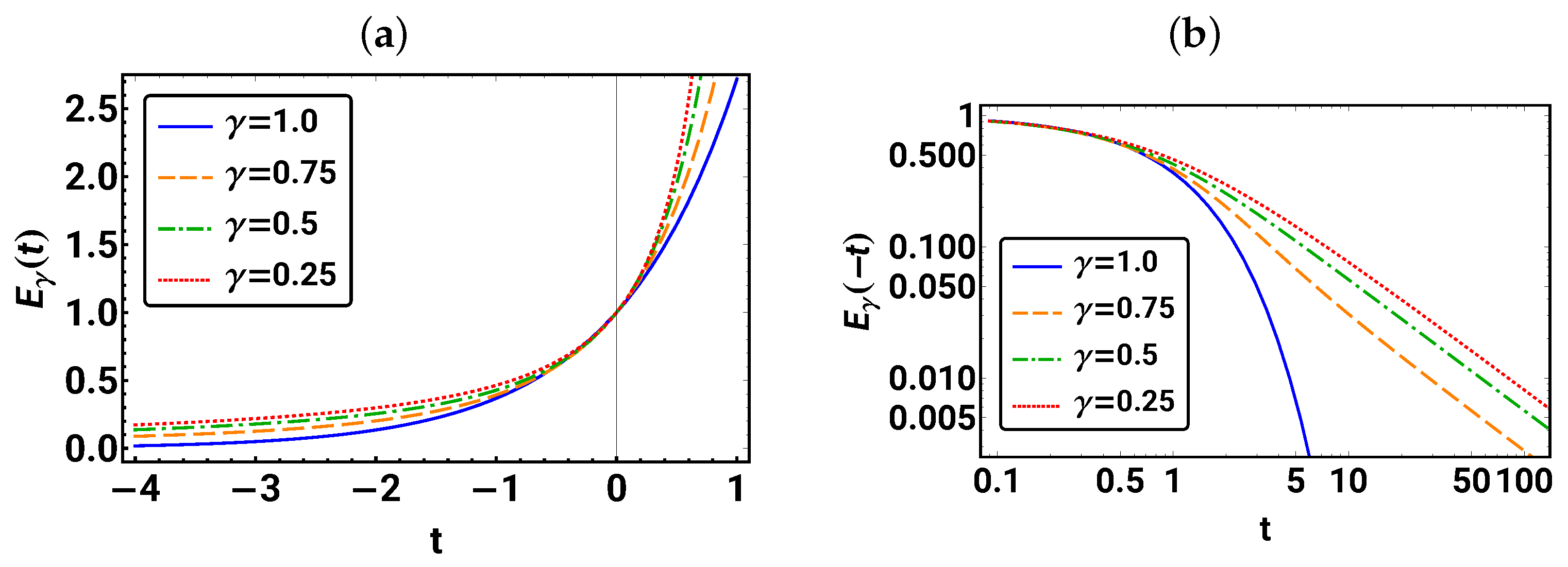
In Figure 1, the resulting plots are shown. For all $\gamma$ values, we observe in Figure 1a monotonic increasing functions $E_{\gamma }\left(t\right)$ that coincide at $t=0$. At this point, $E_{\gamma }\left(0\right)=1$ independent of $\gamma$, a result that can also be found by inserting $t=0$ into Equation (13). Note that in the plot, $E_{{\gamma }_1}\left(t\right)\ge E_{{\gamma }_2}\left(t\right)$ for ${\gamma }_1<{\gamma }_2$ at all t. Furthermore, we observe that for large times, $E_{\gamma }\left(-t\right)$ decreases exponentially towards zero for $\gamma =1$ and as a power law for $\gamma <1$, as indicated by the straight lines for $\gamma <1$ in the double logarithmic-scaled plot in Figure 1b.

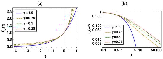
Figure 1. For different values of $\gamma =\{0.25, 0.5, 0.75, 1\}$ in (a), the Mittag–Leffler function $E_{\gamma }\left(t\right)$ is shown for the range $t\in [-4,1]$ and, in (b), the plot of $E_{\gamma }\left(-t\right)$ is given for $t\in [0.1,100]$ on a double logarithmic scale.

We return to the question of whether the Mittag–Leffler function $E_{\gamma }\left(t\right)$ itself is a suitable generalization of $\exp \left(t\right)$, or whether another choice $E_{\gamma }\left(t^{\gamma }\right)$ would be more appropriate. Setting $\gamma =1$, the Mittag–Leffler function $E_{\gamma }\left(t\right)$ itself as well as the modification $E_{\gamma }\left(t^{\gamma }\right)$ clearly return the exponential function. But, it turns out that in order to be compatible with the often used Caputo definition of the fractional derivative  [46,47,48], the appropriate choice is

$$\begin{array}{c}\hfill {\exp }_{\gamma }\left(t\right)=E_{\gamma }\left(t^{\gamma }\right).\end{array}$$

(14)

It represents the identity in Equation (12) and allows a physical interpretation of the modeled process. As the fractional differential operator is—analogous to the classical integer differential operator—a linear operator (see Equation (8)), the solutions to the fractional diffusion equation can be built as sums of suitable terms depending on t as in the classical sense.

Task 2. 

Plot $E_{\gamma }\left(t^{\gamma }\right)$ with $\gamma =\{0.25,0.5,0.75,1\}$ for $t\in [0,1]$. What is the value at $t=0$? Does $E_{\gamma }\left(-t^{\gamma }\right)$ behave similarly to $E_{\gamma }\left(-t\right)$ for larger values of t?

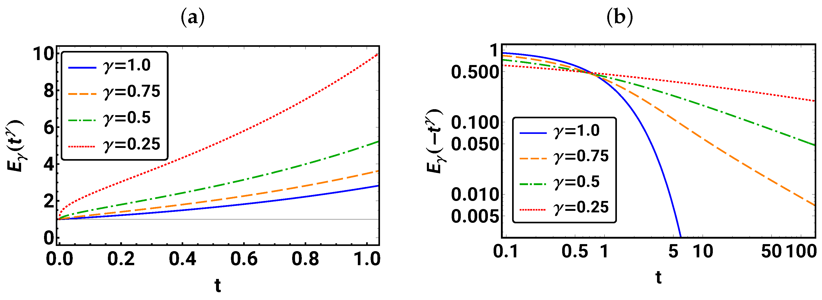
In Figure 2, the resulting plots are shown. In Figure 2a, one can see that, for any fixed t, the values of $E_{\gamma }\left(t^{\gamma }\right)$ increase with decreasing $\gamma$. For all $\gamma$ values, $E_{\gamma }\left(0^{\gamma }\right)=1$. In Figure 2b, we observe monotonic decreasing behavior for all $\gamma$. However, while exponential decay is present for $\gamma =1$, for $\gamma \ne 1$, a power law behavior appears for large enough values of t with stronger decay for larger $\gamma$ values, which is now analyzed in more detail.

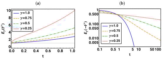
Figure 2. For different values of $\gamma =\{0.25,0.5,0.75,1\}$ in (a), the generalized exponential function ${\exp }_{\gamma }\left(t\right)=E_{\gamma }\left(t^{\gamma }\right)$ is given for the range $t\in [0,1]$ and, in (b), the plot of $E_{\gamma }\left(-t^{\gamma }\right)$ is shown for $t\in [0.1,100]$ on a double logarithmic scale. The horizontal line indicates 1.

For negative Mittag–Leffler arguments, we introduce a new function $e_{\gamma }\left(t\right):=E_{\gamma }\left(-t^{\gamma }\right)$, following [50]. Using (13), we find from the direct substitution of $-t^{\gamma }$ that

$$\begin{array}{c}\hfill e_{\gamma }\left(t\right)=\sum _{k=0}^{\infty }{(-1)}^k{\displaystyle \frac{t^{\gamma k}}{\Gamma (\gamma k+1)}}\mathrm{for}t>0,0<\gamma \le 1.\end{array}$$

(15)

In Figure 2b, we observe $e_{\gamma }\left(t\right)$ is a rapidly decreasing function of t for different values of $\gamma$. The convergent asymptotic form of $e_{\gamma }\left(t\right)$ for large t [50] confirms this:

$$\begin{array}{c}\hfill e_{\gamma }\left(t\right)\sim \sum _{k=1}^{\infty }{(-1)}^{k-1}{\displaystyle \frac{t^{-\gamma k}}{\Gamma (1-\gamma k)}}\mathrm{for}t\to \infty 0<\gamma \le 1.\end{array}$$

(16)

Theorem 1. 

There exists a constant, ξ, such that

$$\begin{array}{c}\hfill {\displaystyle \frac{d}{d\left(\log t\right)}}\log e_{\gamma }\left(t\right)\to \xi \mathrm{for}t\to \infty .\end{array}$$

(17)

Proof. 

Let

$$\begin{array}{c}\hfill f\left(t\right)\equiv \left\{1-{\displaystyle \frac{\Gamma (1-\gamma )}{\Gamma (1-2\gamma )}}{t}^{-\gamma }+{\displaystyle \frac{\Gamma (1-\gamma )}{\Gamma (1-3\gamma )}}{t}^{-2\gamma }-\cdots +{\displaystyle \frac{\Gamma (1-\gamma )}{\Gamma (1-k\gamma )}}{t}^{-(k-1)\gamma }-\cdots \right\}.\end{array}$$

(18)

Thus,

$$\begin{array}{c}\hfill e_{\gamma }\left(t\right)\sim {\displaystyle \frac{t^{-\gamma }}{\Gamma (1-\gamma )}}f\left(t\right).\end{array}$$

(19)

Given that the right side of (16) is convergent for large t,

$$\begin{array}{c}\hfill f\left(t\right)\sim 1\mathrm{for}t\to \infty .\end{array}$$

(20)

Thus, another equally valid asymptotic form for $e_{\gamma }$ for large t is

$$\begin{array}{c}\hfill e_{\gamma }\left(t\right)\sim {\displaystyle \frac{t^{-\gamma }}{\Gamma (1-\gamma )}}.\end{array}$$

(21)

The logarithmic derivative applied to the right side yields $\xi =-\gamma$, which completes the proof.    □

3. Linear Fractional Differential Equations

With the above meaning given to the fractional differentiation operator via the generalized exponential ${\exp }_{\gamma }\left(t\right)$ being its identity and more generally ${\exp }_{\gamma }\left(at\right)$ being the eigenfunction to the eigenvalue a, we now turn to the solution of the fractional differential equation. We start with the simplest case:

Task 3. 

${\displaystyle \frac{{\mathrm{d}}^{\gamma }}{\mathrm{d}{t}^{\gamma }}}$ is a linear operator. Find the solution to

$$\begin{array}{c}\hfill {\displaystyle \frac{{\mathrm{d}}^{\gamma }}{\mathrm{d}{t}^{\gamma }}}y\left(t\right)=y\left(t\right),\end{array}$$

(22)

with initial condition $y\left(0\right)=5b$, with b being a real number.

Above, we found that ${\exp }_{\gamma }\left(0\right)=E_{\gamma }\left(0^{\gamma }\right)=1$. As Equation (22) is a linear equation with a linear fractional differential operator, it follows that Equation (22) only specifies solutions up to a free factor c, i.e., $y\left(t\right)=c{\exp }_{\gamma }\left(t\right)$, requiring the initial value to set a specific function. Thus, we have

$$\begin{array}{c}\hfill y\left(t\right)=5b{\exp }_{\gamma }\left(t\right).\end{array}$$

(23)

The fractional differential Equation (22)—also called an extraordinary differential equation [51,52]—can be modified to produce a slightly more complicated case using a constant a,

$$\begin{array}{c}\hfill {\displaystyle \frac{{\mathrm{d}}^{\gamma }}{\mathrm{d}{t}^{\gamma }}}y\left(t\right)=ay\left(t\right).\end{array}$$

(24)

In order to solve this, we again appeal to the $\gamma =1$ case to guide us. After dividing by a and rearranging, Equation (24) becomes

$$\begin{array}{c}\hfill {\displaystyle \frac{\mathrm{d}}{\mathrm{d}\left(at\right)}}y\left(t\right)=y\left(t\right).\end{array}$$

(25)

The solution $y\left(t\right)=\exp \left(at\right)$ follows from the substitution of $t\to at$ in Equation (9).

Intuitively, following these steps for $\gamma \ne 1$ leads to

$$\begin{array}{c}\hfill {\displaystyle \frac{{\mathrm{d}}^{\gamma }}{\mathrm{d}{\left(a^{1/\gamma }t\right)}^{\gamma }}}y\left(t\right)=y\left(t\right).\end{array}$$

(26)

Thus, a is associated with $t^{\gamma }$ rather than t, and the generalization is not ${\exp }_{\gamma }\left(at\right)$. It suggests that for positive a, the function ${\exp }_{\gamma }\left(a^{1/\gamma }t\right)$ is the solution. More generally, one finds for both positive and negative a that

$$\begin{array}{cc}\hfill y\left(t\right)& =E_{\gamma }\left(a{t}^{\gamma }\right),\hfill \end{array}$$

(27)

as a solution of Equation (24). Thus, one can say that $E_{\gamma }\left(a{t}^{\gamma }\right)$ is an eigenfunction of the operator ${\mathcal{D}}^{\gamma }$ with eigenvalue a:

$$\begin{array}{c}\hfill {\mathcal{D}}^{\gamma }{E}_{\gamma }\left(a{t}^{\gamma }\right)=a{E}_{\gamma }\left(a{t}^{\gamma }\right).\end{array}$$

(28)

4. Discretizing Space

We now return to the time-fractional diffusion equation,

$$\begin{array}{cc}\hfill {\displaystyle \frac{{\partial }^{\gamma }}{\partial t^{\gamma }}}P(x,t)& =D_{\gamma }{\displaystyle \frac{{\partial }^2}{\partial x^2}}P(x,t),\hfill \end{array}$$

(29)

which we want to solve on a finite interval $0<x<\ell$ under the condition that the diffusing particles cannot leave that interval, i.e., the probability in the interval must always be one. This differential equation is not yet in a form where we can make use of the solution to the fractional differential Equation (24). However, we can achieve such a form by discretizing the spatial coordinate x as

$$\begin{array}{c}\hfill x\left(i\right)=(i-1/2)h,\end{array}$$

(30)

with $1\le i\le N$ and $h=\ell /N$. Once that has been performed, the probability of being in an interval between $x\left(i\right)-{\displaystyle \frac{1}{2}}h$ and $x\left(i\right)+{\displaystyle \frac{1}{2}}h$ can be thought of as being collected into $P_i\left(t\right)$ at node i.

Thus, instead of a probability density $P(x,t)$ depending on continuous time t and space x, we now have a probability distribution represented by a vector of probability $\mathbf{P}$ with elements $P_i$ (still depending continuously on time t).

This probability distribution obeys a set of coupled fractional differential equations also known as a fractional master equation [53,54]. In order to obtain the fractional master equation, we replace the second-order space derivative in Equation (29) with a finite difference approximation. Consider truncated power series (Taylor series) approximations for $y(x+h)$ and $y(x-h)$ up to order 4:

$$\begin{array}{cc}\hfill y(x+h)& =y\left(x\right)+y^{\prime }\left(x\right)h+{\displaystyle \frac{y^{″}\left(x\right)h^2}{2}}+{\displaystyle \frac{y^{‴}\left(x\right)h^3}{6}}+\mathcal{O}\left(h^4\right)\mathrm{and}\hfill \end{array}$$

(31)

$$\begin{array}{cc}\hfill y(x-h)& =y\left(x\right)-y^{\prime }\left(x\right)h+{\displaystyle \frac{y^{″}\left(x\right)h^2}{2}}-{\displaystyle \frac{y^{‴}\left(x\right)h^3}{6}}+\mathcal{O}\left(h^4\right).\hfill \end{array}$$

(32)

Adding these two equations leads to

$$\begin{array}{c}\hfill y(x+h)+y(x-h)=2y\left(x\right)+y^{″}\left(x\right)h^2+\mathcal{O}\left(h^4\right),\end{array}$$

(33)

and thus we arrive at the central difference formula:

$$\begin{array}{c}\hfill y^{″}\left(x\right)={\displaystyle \frac{y(x+h)+y(x-h)-2y\left(x\right)}{h^2}}+\mathcal{O}\left(h^2\right).\end{array}$$

(34)

Applying this approximation to Equation (29), one obtains for the inner nodes, i.e., $1<i<N$

$$\begin{array}{c}\hfill {\displaystyle \frac{{\mathrm{d}}^{\gamma }}{\mathrm{d}{t}^{\gamma }}}{P}_i\left(t\right)\approx {\displaystyle \frac{D_{\gamma }}{h^2}}\left(P_{i-1}\left(t\right)-2P_i\left(t\right)+P_{i+1}\left(t\right)\right).\end{array}$$

(35)

For the boundary nodes, $i=1$ and $i=N$, Equation (35) is modified for the two cases:

$${\displaystyle \frac{{\mathrm{d}}^{\gamma }}{\mathrm{d}{t}^{\gamma }}}{P}_1\left(t\right)\approx {\displaystyle \frac{D_{\gamma }}{h^2}}\left(-P_1\left(t\right)+P_2\left(t\right)\right)\mathrm{and}$$

(36)

$${\displaystyle \frac{{\mathrm{d}}^{\gamma }}{\mathrm{d}{t}^{\gamma }}}{P}_N\left(t\right)\approx {\displaystyle \frac{D_{\gamma }}{h^2}}\left(-P_N\left(t\right)+P_{N-1}\left(t\right)\right).$$

(37)

They represent reflecting boundaries, i.e., no probability can leave the interval.

The above considerations lead to the following set of coupled fractional differential equations for probabilities $P_i\left(t\right)$, which can be written in a matrix vector form as

$$\begin{array}{c}\hfill {\displaystyle \frac{{\mathrm{d}}^{\gamma }}{\mathrm{d}{t}^{\gamma }}}\mathbf{P}\left(t\right)=\mathcal{W}\mathbf{P}\left(t\right)\end{array}$$

(38)

with the matrix

$$\mathcal{W}=\kappa \left(\begin{array}{ccccccc}\hfill -1& \hfill 1& \hfill 0& \hfill 0& \hfill 0& \hfill \cdots & \hfill 0\\ \hfill 1& \hfill -2& \hfill 1& \hfill 0& \hfill 0& \hfill \cdots & \hfill 0\\ \hfill 0& \hfill 1& \hfill -2& \hfill 1& \hfill 0& \hfill \cdots & \hfill 0\\ \hfill & \hfill & \hfill & \hfill \ddots & \hfill & \hfill & \hfill \\ \hfill 0& \hfill \cdots & \hfill 0& \hfill 1& \hfill -2& \hfill 1& \hfill 0\\ \hfill 0& \hfill \cdots & \hfill 0& \hfill 0& \hfill 1& \hfill -2& \hfill 1\\ \hfill 0& \hfill \cdots & \hfill 0& \hfill 0& \hfill 0& \hfill 1& \hfill -1\end{array}\right),$$

(39)

where $\kappa =D_{\gamma }/h^2$, which thus has the unit [time^γ]. With an appropriate choice of the time unit, one can always set $\kappa =1$. Note that the probability $\mathbf{P}$ is an element in a vector space of N tuples.

Similar to decoupling a set of coupled ordinary linear differential equations and as the fractional derivative is a linear operator too, the coupled set of fractional differential equations can be decoupled by diagonalizing the matrix $\mathcal{W}$.

Task 4. 

Determine the eigenvalues ${\lambda }_{\nu }$ and corresponding eigenvectors ${\mathbf{v}}^{\nu }$ of matrix $\mathcal{W}$ for $N=5$, and plot the eigenvector elements $v_i^{\nu }$ as a function of i.

(1) 

What are the eigenvalues of $\mathcal{W}$?

(2) 

Does the matrix $\mathcal{W}$ have different left and right eigenvectors?

(3) 

Are the eigenvectors orthogonal? Note, that a left eigenvector of matrix $\mathcal{W}$ is the right eigenvector of ${\mathcal{W}}^{\mathrm{T}}$.

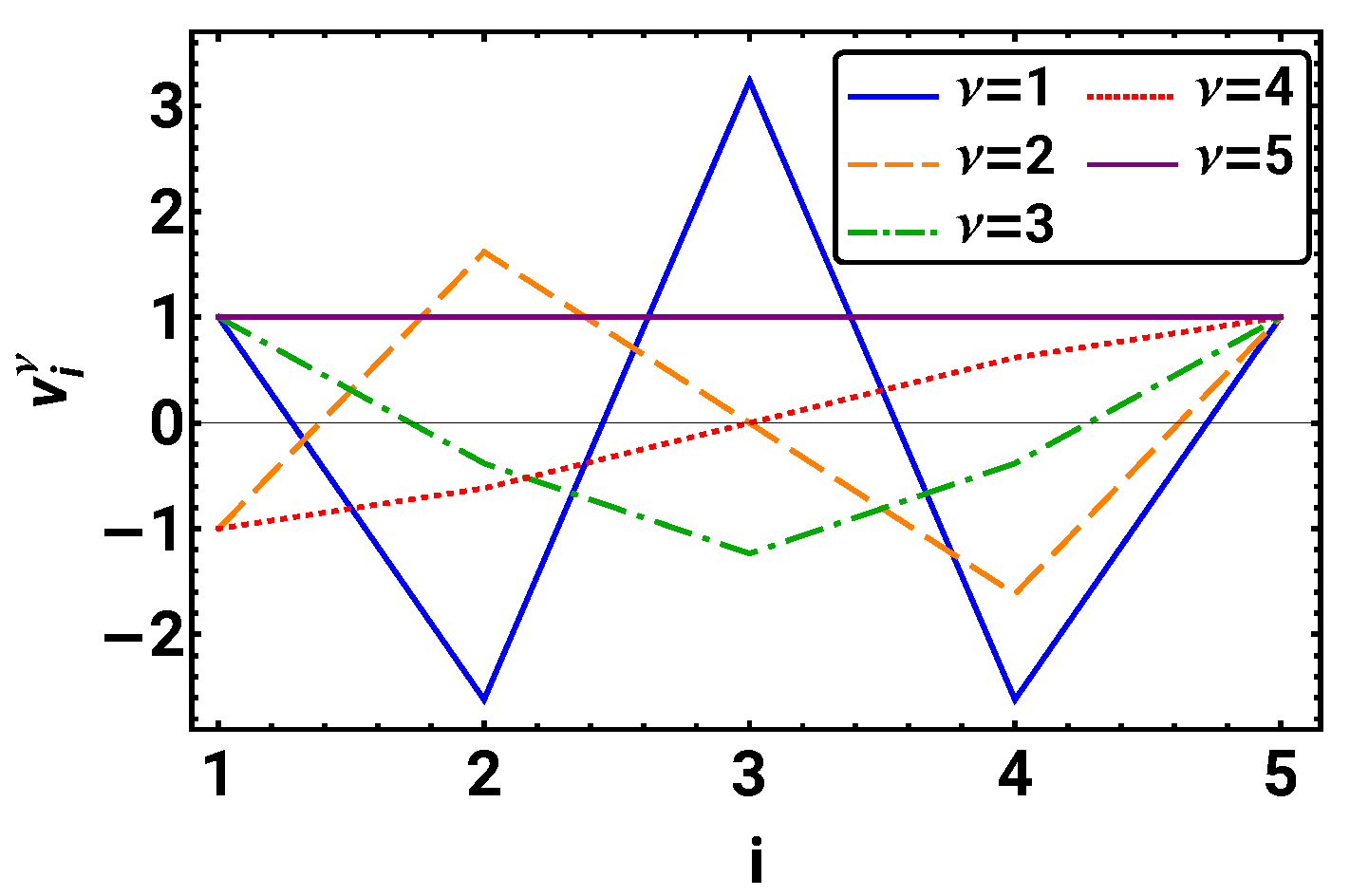
The eigenvalues ${\lambda }_{\nu }$ and eigenvectors ${\mathbf{v}}^{\nu }$ are determined using the MATHEMATICA command Eigensystem[$\mathcal{W}$]. We find that the eigenvalues are all different and ≤0. We can sort them such that ${\lambda }_{\nu -1}<{\lambda }_{\nu }$ and ${\lambda }_N=0$ to give each eigenvalue and eigenvector a unique labeling. Figure 3 gives the resulting sorted eigenvectors of $\mathcal{W}$. We observe that the eigenvector to the largest eigenvalue ${\lambda }_5$ is a constant vector with ${\sum }_i{v}_i^5=5$. For eigenvectors $\nu \ne N$, we obtain ${\sum }_i{v}_i^{\nu \ne N}=0$ (within numerical precision), where the eigenvectors with $\nu =2k$ and $k=1,2,\cdots$—even eigenvectors—are antisymmetric with respect to the midpoint $i=(N+1)/2$, and the eigenvectors with $\nu =2k+1$ and $k=1,2,\cdots$—odd eigenvectors—are mirror-symmetric with respect to the midpoint.

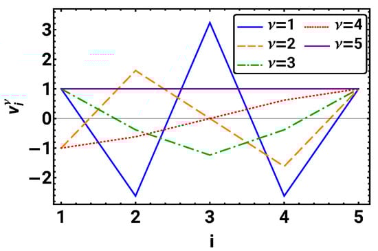
Figure 3. The five eigenvectors ${\mathbf{v}}^{\nu }$ of matrix $\mathcal{W}$ with $N=5$ are shown. They are sorted by their eigenvalues ${\lambda }_{\nu }$ such that ${\lambda }_{\nu -1}<{\lambda }_{\nu }$ and ${\lambda }_5=0$.

As the matrix $\mathcal{W}$ is symmetric, the left and right eigenvectors are the same. From this and the uniqueness of each eigenvalue, we can conclude that all the eigenvectors are orthogonal to each other.

Task 5. 

Check this by computing matrix $\mathcal{T}$ with $T_{\nu ,\mu }={\mathbf{v}}^{\nu }·{\mathbf{v}}^{\mu }$ for $\nu \ne \mu$. Its elements should all be zero (or less than machine precision).

The orthogonal eigenvectors form a basis in the vector space of N tuples, and thus the probability vector $\mathbf{P}$ can be written as a linear combination of the eigenvectors,

$$\begin{array}{cc}\hfill \mathbf{P}\left(t\right)& =\sum _{\nu =1}^N{a}_{\nu }\left(t\right){\mathbf{v}}^{\nu },\hfill \end{array}$$

(40)

where the coefficients $a_{\nu }\left(t\right)$ are time-dependent.

In order to express the time-dependent coefficients $a_{\nu }\left(t\right)$ in terms of a given probability distribution $\mathbf{P}\left(t\right)$, we take the scalar product of ${\mathbf{v}}^{\mu }$ and Equation (40). We find that

$${\mathbf{v}}^{\mu }·\mathbf{P}\left(t\right)=\sum _{\nu }{a}_{\nu }\left(t\right){\mathbf{v}}^{\mu }·{\mathbf{v}}^{\nu }$$

(41)

$$\begin{array}{cc}\hfill & =a_{\mu }\left(t\right){\mathbf{v}}^{\mu }·{\mathbf{v}}^{\mu }\hfill \end{array}$$

(42)

due to the orthogonality of the eigenvectors. In particular, the coefficients for the initial probability distribution $\mathbf{P}\left(0\right)={\mathbf{P}}^0$ are

$$\begin{array}{c}\hfill a_{\mu }^0={\displaystyle \frac{{\mathbf{v}}^{\mu }·{\mathbf{P}}^0}{{\mathbf{v}}^{\mu }·{\mathbf{v}}^{\mu }}}.\end{array}$$

(43)

Inserting the linear combination (40) into the space-discretized time-fractional diffusion Equation (38) and taking the scalar product of ${\mathbf{v}}^{\mu }$ with it, we find

$${\displaystyle \frac{{\mathrm{d}}^{\gamma }}{\mathrm{d}{t}^{\gamma }}}{a}_{\mu }\left(t\right)={\lambda }_{\mu }{a}_{\mu }\left(t\right).$$

(44)

Thus, we obtain a set of decoupled time-fractional differential Equations (44) for coefficients $a_{\mu }\left(t\right)$ with initial conditions $a_{\mu }\left(0\right)=a_{\mu }^0$ taken from (43). Now, one can make use of the known solution to these fractional differential equations derived in Section 3.

Task 6. 

For $N=5$, determine coefficients $a_{\mu }^0$ for initial distribution $P_i^0={\delta }_{i,3}$, where ${\delta }_{i,j}=1$ for $i=j$ and ${\delta }_{i,j}=0$ for $i\ne j$. Then, use these to calculate ${\mathbf{w}}^{\mu }=a_{\mu }^0{\mathbf{v}}^{\mu }$ and, based on those, the resulting $\mathbf{P}\left(t\right)$.

$a_{\mu }^0$ are generated using Equation (43). Then, the vector $\mathbf{P}\left(t\right)$ is determined by

$$\mathbf{P}(t)=\sum _{\nu }{a}_{\nu }^0{E}_{\gamma }\left({\lambda }_{\nu }{t}^{\gamma }\right){\mathbf{v}}^{\nu }$$

(45)

$$\begin{array}{cc}\hfill & =\sum _{\nu }{E}_{\gamma }\left({\lambda }_{\nu }{t}^{\gamma }\right){\mathbf{w}}^{\nu },\hfill \end{array}$$

(46)

representing a solution of Equation (44) for the given initial conditions. This solution consists of time- and space-dependent factors. Note that for $\gamma =1$, this equation reduces to the typical exponential form

$$\mathbf{P}(t)=\sum _{\nu }\exp \left({\lambda }_{\nu }t\right){\mathbf{w}}^{\nu }.$$

(47)

Following the standard nomenclature for linear systems, we refer to a single term of the sum in (46) and (47) as a mode, with its temporal behavior given by $a_{\nu }^0{E}_{\gamma }\left({\lambda }_{\nu }{t}^{\gamma }\right)$ and its spatial features by ${\mathbf{v}}^{\nu }$. Below, we show that thinking of the solution $\mathbf{P}\left(t\right)$ as a composition of modes gives a good framework for an intuitive understanding of its dynamics.

5. Temporal Features of Fractional Diffusion on a Finite Interval

Now that we have found the general time-dependent solution $\mathbf{P}\left(t\right)$ (Equation (46)) for the fractional master Equation (38), we are interested in its temporal and spatial features. Our special focus is on the resulting time dependence of the mean square displacement $⟨{(i-i_0)}^2⟩$ introduced in the beginning as well as on the changes in the shape of the distribution over time. We begin with the time development of distribution $\mathbf{P}\left(t\right)$.

Task 7. 

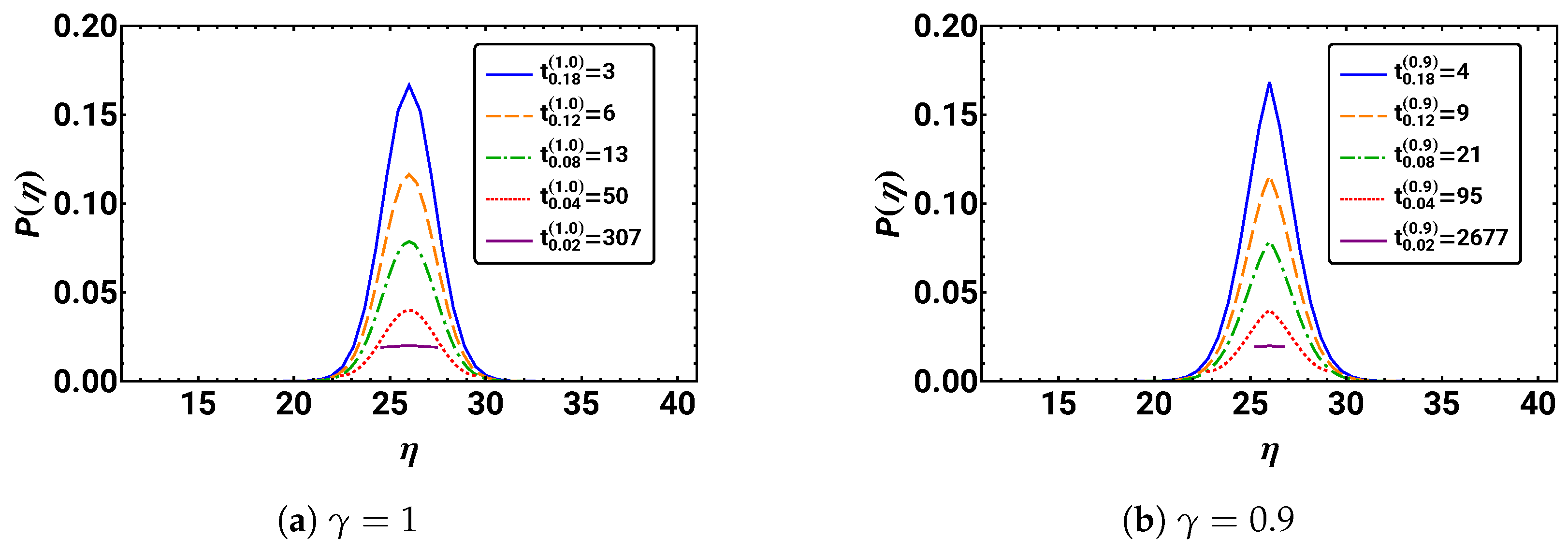
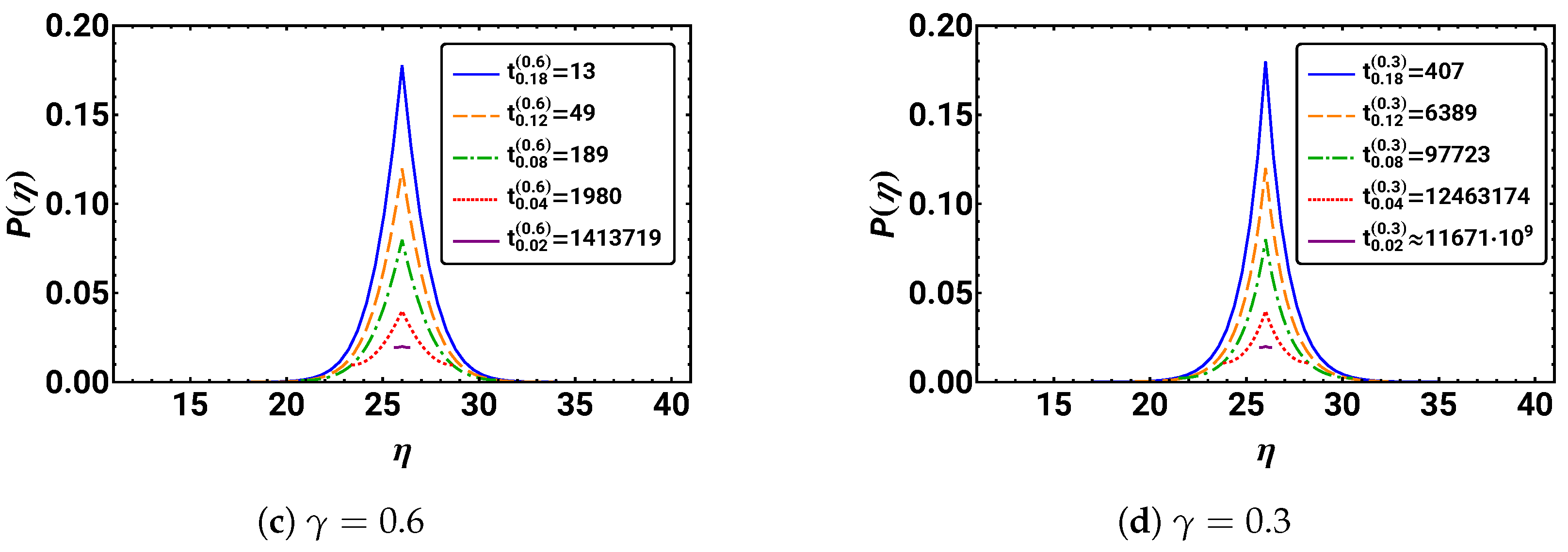
Determine the probability distribution $\mathbf{P}\left(t\right)$ for $N=51$ using the initial condition $\mathbf{P}\left(0\right)={\delta }_{i,i_0}$ with $i_0=26$. Plot the distribution $\mathbf{P}\left(t\right)$ for the regular diffusion case ($\gamma =1$) and the three subdiffusive cases ($\gamma =\{0.9,0.6,0.3\}$), each at five different integer times. In order to obtain plots, which can easily be compared, first determine the times $t_m^{\left(\gamma \right)}$ depending on γ such that $P_{26}(t_m^{\left(\gamma \right)})=m$ for $m\in \{0.18,0.12,0.08,0.04,0.02\}$. Hint: $t_m^{\left(\gamma \right)}$ can be extracted using the MATHEMATICA command FindRoot. Are there any symmetry features? How does the distribution change over time?

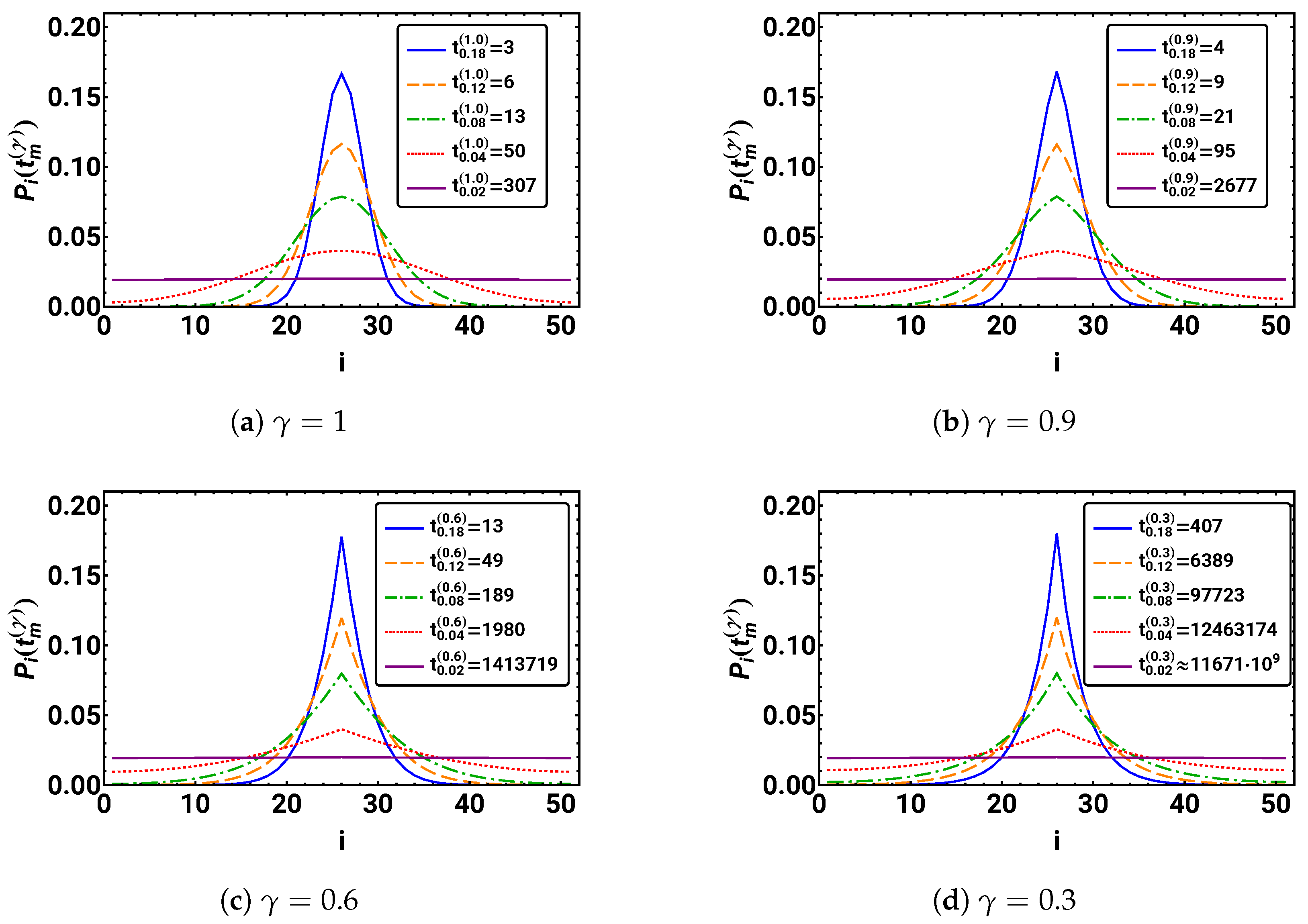
In Figure 4, the resulting plots are given. In the case of regular diffusion, i.e., $\gamma =1$, we observe a Gaussian-like distribution with its maximum at the starting position $i_0=26$, which is stretched and flattened over time. This is similar in the cases of subdiffusion, i.e., $\gamma <1$. However, all distributions keep their sharp peak at the starting position $i_0$. In addition, all distributions appear to be symmetric with respect to an inversion at their peak position $i_0=26$.

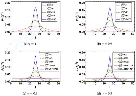
Figure 4. For $\gamma =\{1.0,0.9,0.6,0.3\}$, the probability distributions $\mathbf{P}\left(t\right)$ are depicted for five different times $t_m^{\left(\gamma \right)}$, where $P_{26}\left(t_m^{\left(\gamma \right)}\right)=\{0.18,0.12,0.08,0.04,0.02\}$. The exact value of $t_{0.02}^{\left(0.3\right)}$ = 11 671 630 915 231. For $\gamma =1$, a discretized Gaussian distribution can be observed for all times that becomes smoother as N increases, whereas for smaller $\gamma$, the distributions are spikier. For $\gamma <1$, the kink in the distribution at the starting position $i_0$ is present at all five times.

We recognize that smaller $\gamma$ values correspond to slower spreading of the distributions over space. This is indicated by the different times at which the distributions achieve comparable maximum values. One can see this in the impressive increase in $t_{0.02}^{\left(\gamma \right)}$ = {304, 2677, 1 413 719, 11 671 630 915 231} with $\gamma$. The plots also reveal that the form of the distributions with roughly equal heights approach a Gaussian distribution for $\gamma$ increasing to one. For long durations, all distributions seem to approach the same uniform distribution, where all $P_i(\infty )={\displaystyle \frac{1}{51}}\approx 0.019$.

We note that such an approach to a uniform distribution would not be observed on an unrestricted space.

5.1. Time Development of Mean Square Displacement

In the Introduction, the defining property of anomalous diffusion (6) requires the mean square displacement to increase with a power law with an exponent smaller than one for the subdiffusive case. Moreover, the claim is that fractional diffusion equations are particularly well suited for describing such behavior. Thus, we now turn to the time development of mean square displacement $⟨{(i-i_0)}^2⟩\left(t\right)={\sigma }^2\left(t\right)$ of distribution $\mathbf{P}\left(t\right)$ and analyze its behavior to see whether this is indeed the case.

Task 8. 

Compute the mean square displacement $⟨{(i-i_0)}^2⟩\left(t\right)$ of distribution $\mathbf{P}\left(t\right)$ for $\gamma =\{1.0,0.9,0.6,0.3\}$ for times between 0 and 2000. Describe the shape of the overall curve and discuss the potentially appearing time regimes. Hint for MATHEMATICA users: tabulate the MSD for discrete times, and use the MATHEMATICA command ListPlot.

The mean square displacement of $\mathbf{P}\left(t\right)$ is determined by computing

$$⟨{(i-i_0)}^2⟩\left(t\right)=\sum _{i=1}^N{P}_i\left(t\right){(i-i_0)}^2,$$

(48)

$$\begin{array}{cc}\hfill & =\sum _{i=1}^N\sum _{\nu =1}^N{E}_{\gamma }\left({\lambda }_{\nu }{t}^{\gamma }\right)w_i^{\nu }{(i-i_0)}^2.\hfill \end{array}$$

(49)

We note that one can speed up the computation considerably by performing the i sum first and storing the results for each $\nu$.

An overall plot of the time development of mean square displacement for different values of $\gamma$ is shown in Figure 5. The figure indicates similar behavior in all four cases. First, the variance increases monotonically with decreasing slope. Then, it changes to approach its stationary value in an asymptotic fashion. Comparing the different $\gamma$ values, one can observe that the smaller $\gamma$, the slower $⟨{(i-i_0)}^2⟩$ increases, i.e., the more subdiffusive the process. This is of course a consequence of the slower spreading of the distribution for smaller values of $\gamma$.

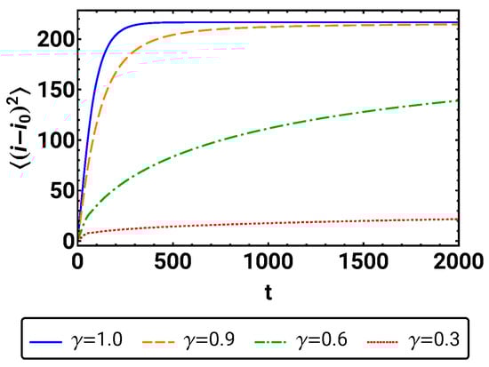
Figure 5. The overall time development of the mean square displacement $⟨{(i-i_0)}^2⟩$ is given for $\gamma =\{1.0,0.9,0.6,0.3\}$.

Obviously, the mean square displacement does not show power law behavior for all times. This, however, should not come as a surprise, as the finiteness of the spatial domain makes it clear from the outset that the mean square displacement is bounded and can thus not grow without limit. So the question remains, whether there is a power law present at small times when the mean square displacement is still increasing.

Task 9. 

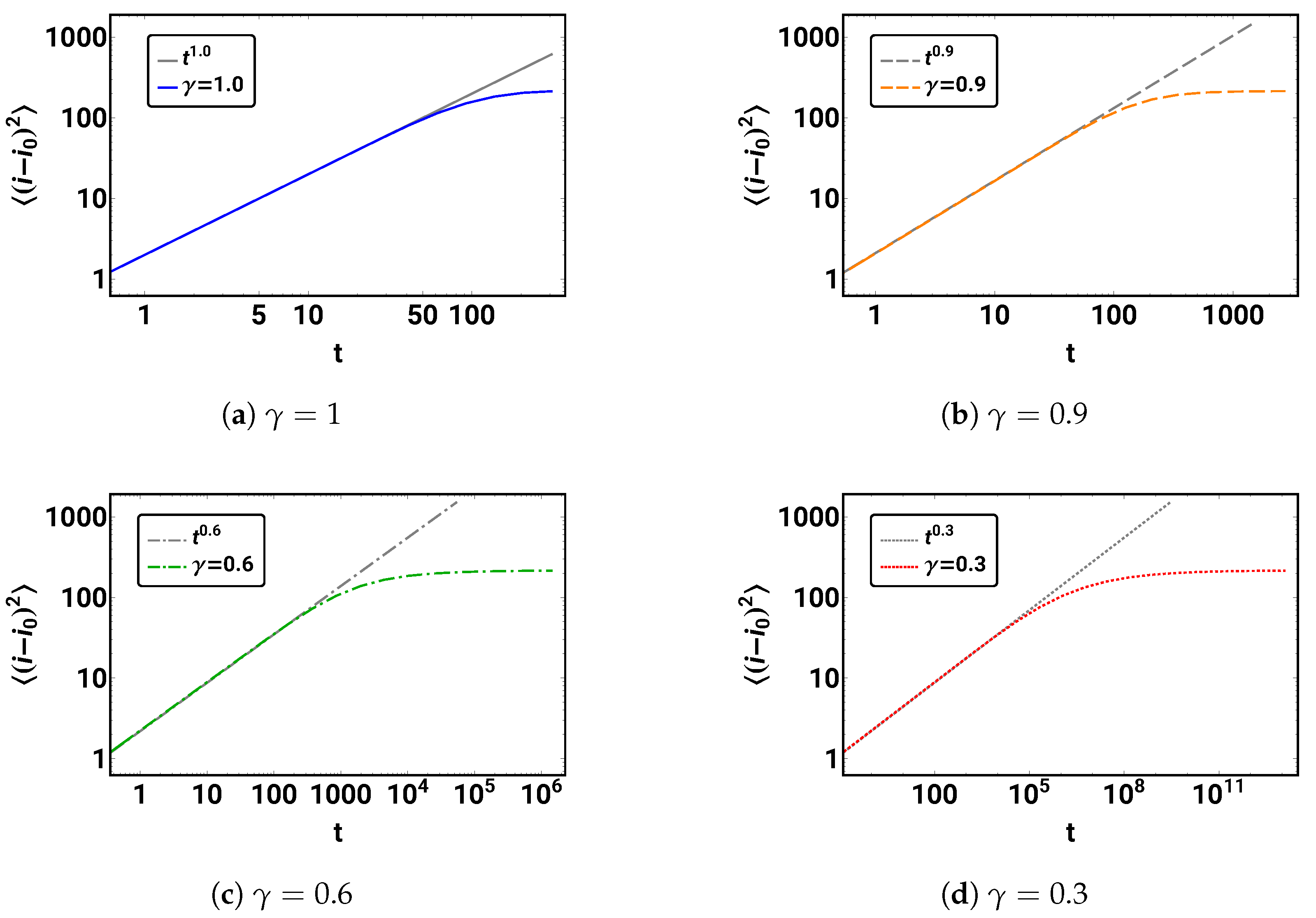
Compute the mean square displacement $⟨{(i-i_0)}^2⟩\left(t\right)$ of the distribution for $\gamma =\{1.0,0.9,0.6,0.3\}$ in the time range of $t=1$ to $t=t_{0.02}^{\left(\gamma \right)}$ and plot it for each γ separately in a log–log plot. In each plot, show the power law tangent for the initial time development. Hint for MATHEMATICA users: use $t=2^j$ with $j=-2,-1,\cdots$ for ListLogLogPlot.

The resulting plots are shown in Figure 6. If a power law is present,

$$\begin{array}{cc}\hfill ⟨{(i-i_0)}^2⟩\left(t\right)& \propto t^{\alpha },\hfill \\ \hfill \log \left(⟨{(i-i_0)}^2⟩\left(t\right)\right)& \propto \alpha \log t,\hfill \end{array}$$

(50)

we would expect a straight line with slope $\alpha$. As indicated by plotting the power laws obtained from Equation (50) and using the corresponding $\gamma$, also given in Figure 6, the variance does indeed show power law behavior with the appropriate exponent $\gamma$ during the initial phase of the time development.

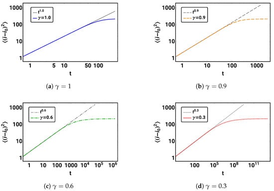
Figure 6. The initial power law behavior of the mean square displacement $⟨{(i-i_0)}^2⟩$ as a function of time (see Equation (50)) is demonstrated for $\gamma =\{1.0,0.9,0.6,0.3\}$. The gray lines show the pure power law, while the colored curves represent the MSD. Note the different time scales for the different values of $\gamma$.

As already discussed above, this power law increase represents the expected time development on an unrestricted domain for both normal diffusion ($\gamma =1$ cf. Equation (5)) and anomalous diffusion ($\gamma <1$ cf. Equation (6)). The observed deviations of the time development of $⟨{(i-i_0)}^2⟩$ from the power law behavior starts as soon as the tails “feel” the boundaries of the finite domain. At this point, the crossover to the final stationary distribution can be observed. Now, a very interesting feature of anomalous diffusion on a finite domain is how the stationary value for the mean square displacement is approached.

For this analysis, it is useful to look at the mode decomposition of the mean square displacement of $\mathbf{P}\left(t\right)$, as determined in Equations (46) and (49).

$$⟨{(i-i_0)}^2⟩\left(t\right)=\sum _{i=1}^N\sum _{\nu =1}^N{E}_{\gamma }\left({\lambda }_{\nu }{t}^{\gamma }\right)w_i^{\nu }{(i-i_0)}^2$$

(51)

$$\begin{array}{cc}\hfill & =\sum _{\nu =1}^N\sum _{i=1}^N{E}_{\gamma }\left({\lambda }_{\nu }{t}^{\gamma }\right)w_i^{\nu }{(i-i_0)}^2\hfill \end{array}$$

(52)

$$\begin{array}{cc}\hfill & =\sum _{\nu =1}^N{⟨{(i-i_0)}^2⟩}_{\nu }\left(t\right),\hfill \end{array}$$

(53)

where

$$\begin{array}{cc}\hfill {⟨{(i-i_0)}^2⟩}_{\nu }\left(t\right)& =E_{\gamma }\left({\lambda }_{\nu }{t}^{\gamma }\right)\sum _{i=1}^N{w}_i^{\nu }{(i-i_0)}^2\hfill \end{array}$$

(54)

is the mean square displacement of mode $\nu$ or—shorter—the mode variance, and $E_{\gamma }\left({\lambda }_{\nu }{t}^{\gamma }\right)$ and

$$r_{\nu }=\sum _i{w}_i^{\nu }{(i-i_0)}^2$$

(55)

are its temporal and spatial parts, respectively.

Recalling Task 4, we found that all even eigenvectors for $\nu \ne N$ are antisymmetric under reflection at $i_0$. $r_{\nu }$ indicates the mirror symmetry of the initial distribution around $i=26$; thus, all spatial parts of the even modes vanish and all even modes of the mean square distribution are 0.

Furthermore, all eigenvalues are negative, apart from ${\lambda }_{N=51}=0$. This property of the eigenvalues leads, for all odd mode variances ${⟨{(i-i_0)}^2⟩}_{\nu }\left(t\right)$ with $\nu \ne 51$ to a power law or exponential ($\gamma =1$) decay towards zero as ${\lim }_{t\to \infty }{E}_{\gamma }\left({\lambda }_{\nu }{t}^{\gamma }\right)=0$.

From the variance (cf. Figure 5), we can find that the slower $E_{\gamma }\left(t^{\gamma }\right)$ decreases, the smaller $\gamma$ is, but, if one waits long enough, all temporal modes, except the constant one ($\nu =51$), disappear. For $\nu =51$, the mode variance is constant over time. We now look at the implications of these findings.

Task 10. 

What is the stationary value of the mean square displacement (or variance)? (Hint: look at the mode separation of $\mathbf{P}\left(t\right)$).

Using the mode decomposition Equation (53), one obtains the long-term behavior for normal and anomalous diffusion on a finite line with reflecting boundary conditions as

$$\underset{t\to \infty }{\lim }⟨{(i-i_0)}^2⟩\left(t\right)=\sum _{i=1}^N{w}_i^N{(i-i_0)}^2,$$

(56)

which is independent of $\gamma$. For the given example, ${\lim }_{t\to \infty }⟨{(i-i_0)}^2⟩\left(t\right)={\displaystyle \frac{650}{3}}\approx 216.667$, as presented in Figure 5 for $\gamma =1.0$ and $0.9$.

The next question we want to answer regards the functional form in which $⟨{(i-i_0)}^2⟩\left(t\right)$ approaches its stationary value. In order to find the answer, we first look at the mode variances.

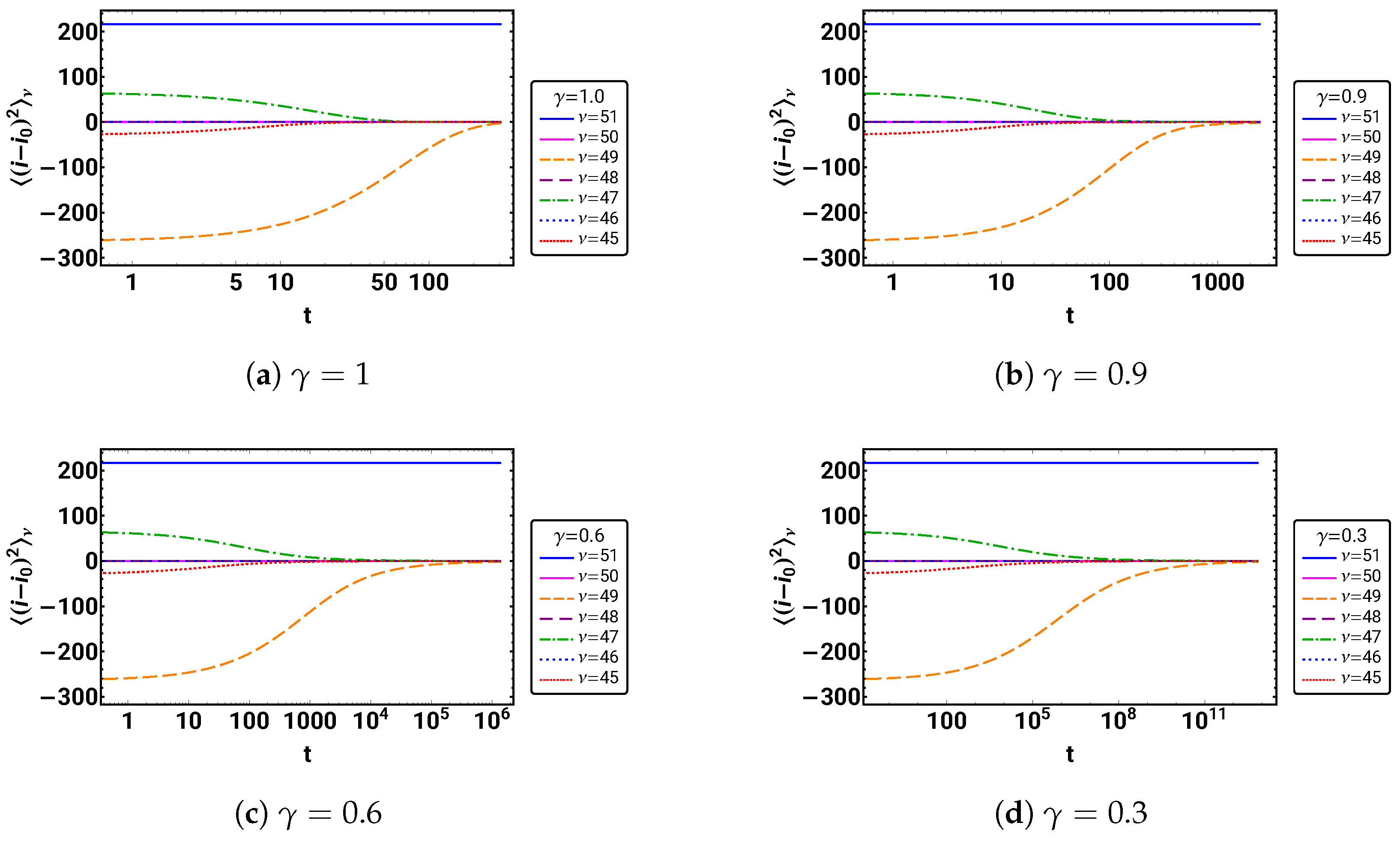
Task 11. 

Plot the mode variances ${⟨{(i-i_0)}^2⟩}_{\nu }$ for $45\le \nu \le 51$ as a function of logarithmic time ($1\le t\le t_{0.02}^{\left(\gamma \right)}$) for each $\gamma =\{1.0,0.9,0.6,0.3\}$ separately.

Figure 7 shows the temporal behavior of the mode variances.

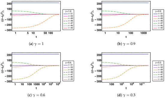
Figure 7. The logarithmic time development of the modevvariances ${⟨{(i-i_0)}^2⟩}_{\nu }$ for $\nu =\{51,\cdots ,45\}$ and $\gamma =\{1.0,0.9,0.6,0.3\}$. Note that for even $\nu$, ${⟨{(i-i_0)}^2⟩}_{\nu }=0$.

As expected, all even mode variances are zero, and, due to the chosen ordering of the eigenvalues, the larger the $\nu$, the longer it takes for the odd ones to decay (apart from the stationary one). One can then expect that with increasing time, fewer and fewer of the mode variances contribute to the overall mean square displacement.

In order to study the terminal approach to its stationary value, we use the folowing:

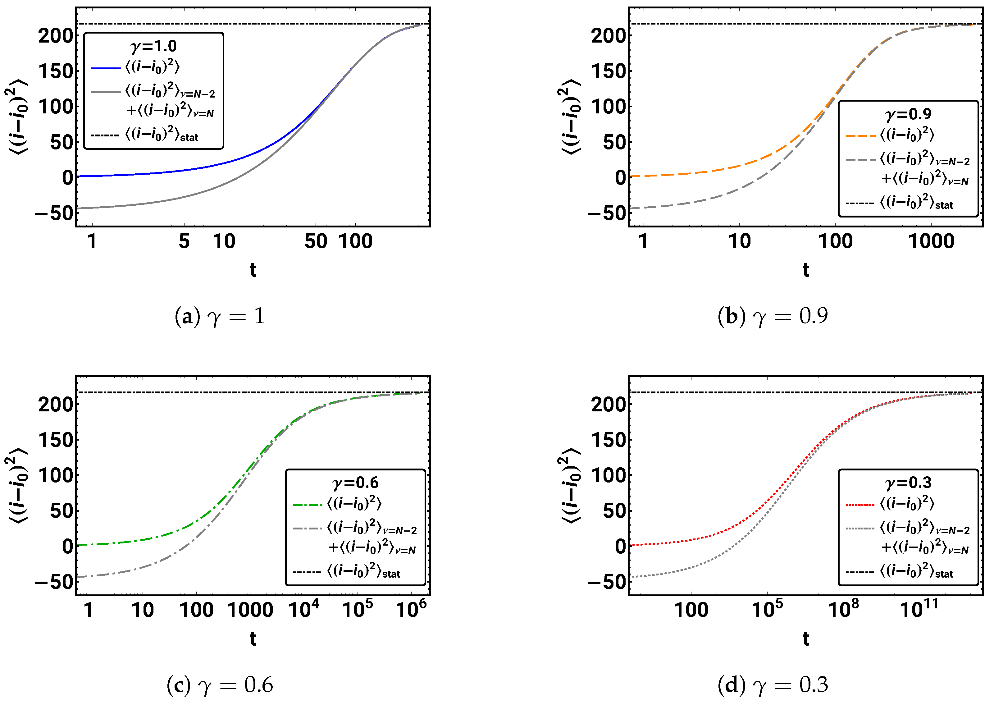
Task 12. 

Plot the mean square displacement $⟨{(i-i_0)}^2⟩$, the stationary mode variance ${⟨{(i-i_0)}^2⟩}_N$, and ${⟨{(i-i_0)}^2⟩}_N+{⟨{(i-i_0)}^2⟩}_{N-2}$ as a function of time ($1\le t\le t_{0.02}^{\left(\gamma \right)}$) for each $\gamma =\{1.0,0.9,0.6,0.3\}$ separately.

Figure 8 shows the resulting variances.

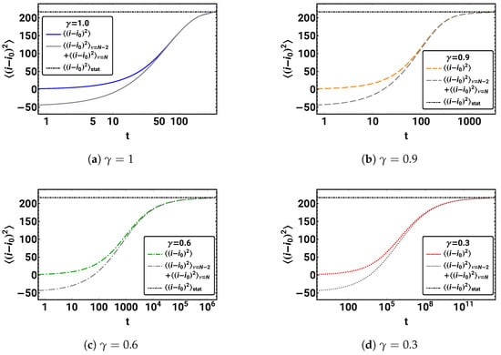
Figure 8. The transition behavior of the mean square displacement $⟨{(i-i_0)}^2⟩$ to the stationary regime, the two-mode approximation, and the stationary value is shown for $\gamma =\{1.0,0.9,0.6,0.3\}$. Despite the different time scales, the graphs’ shapes are quite similar. Note that the negative values of the two-mode approximation for short times result from the missing modes ${⟨{(i-i_0)}^2⟩}_{\nu }$ for $\nu <N-2$.

One finds that the functional form with which the stationary value is finally reached is determined by the slowest decaying mode. In the case of our symmetric initial distribution, this is the $(N-2)$ mode; in general, this would be the $(N-1)$ mode of the mean square displacement. Thus, the functional form for the final approach to the stationary value is

$$\begin{array}{c}\hfill ⟨{(i-i_0)}^2⟩\approx {⟨{(i-i_0)}^2⟩}_N+{⟨{(i-i_0)}^2⟩}_{N-2},\end{array}$$

(57)

which we refer to as two-mode approximation.

Overall, we find that the initial time regime of the mean square displacement is very well approximated by power law behavior (see Equation (50)), and the transition to the stationary value is given by the two-mode approximation (see Equation (57)). Depending on $\gamma$, there exists a transition regime between the initial power law increase and the final two-mode approximation in which fewer and fewer modes are still important.

5.2. Similarity Approach—Rescaling the Probability Distribution

In the following, we investigate changes in the shape of the distributions as they evolve over time. In particular, we are interested in the similarities between the distributions for different times, which are shown in Figure 4. Somehow, the distributions seem to be stretched along the i-axis and to be squished (better: shrunk) along the P-axis.

We first look at the stretching. In the previous discussion of the mean square displacement we observed its initial power law behavior given in Equation (50). This behavior suggests that the distance from the origin of the diffusion at $i_0$ to an equivalent position i increases with $t^{\gamma /2}$, and thus a new variable, $\eta (i,t)=(i-i_0)/t^{\gamma /2}+i_0$, should rescale the distances from $i_0$ such that the ongoing stretching is compensated, and the distributions are squashed back.

Task 13. 

Create parametric plots of probabilities $P_i\left(t\right)$ over the suggested variable $\eta (i,t)$ as a function of $1\le i\le 51$ for $\gamma =\{1.0,0.9,0.6,0.3\}$. For comparison, choose the same times as in Task 7.

The resulting plots, Figure 9, show that the anticipated scaling properties initially work, i.e., until the probability distribution reaches the boundaries of the system. The distributions now are roughly non-zero on the same $\eta$ domain. Also, the shape of the distributions look the same for the different times.

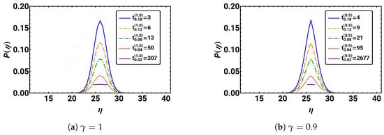
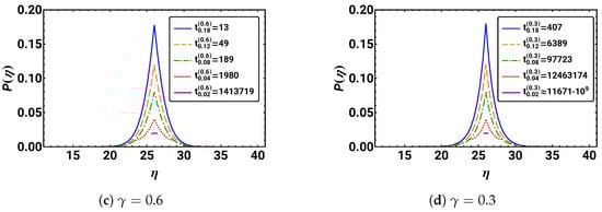
Figure 9. The rescaled, but not normalized, distributions $\mathbf{P}\left(\eta \right)$ for the same times as in Figure 4 are given over the scaling variable $\eta$ for different values of $\gamma$. We see that the rescaling only works for the initial time regime.

However, the resulting distributions $\mathbf{P}\left(\eta \right)$ are of different heights, and thus we have to deal with the shrinking and its time dependence. Due to the compensation of the stretching, the point density in $\eta$ increased and has to be compensated too. Consider a rectangle that is squashed in width by a factor of two; then, in order to keep its area, one should stretch it by a factor of two in height. It thus seems to be a good guess that multiplying $P_i\left(t\right)$ by stretching factor $t^{\gamma /2}$ compensates for our squashing and thus keeps the normalization correct.

This can be formalized: let $P(i,t)$ be a probability density depending on continuous i and t. Normalization on the real axis requires

$$\begin{array}{c}\hfill \int P(i,t)\mathrm{d}i=1.\end{array}$$

(58)

If we stretch that density by a factor a in i and call the result $\widehat{P}(i,t)=P(ai,t)$, then

$$\begin{array}{c}\hfill \int \widehat{P}(i,t)\mathrm{d}i=\int P(ai,t)\mathrm{d}i={\displaystyle \frac{1}{a}}\int P(ai,t)\mathrm{d}\left(ai\right)={\displaystyle \frac{1}{a}}.\end{array}$$

(59)

Thus, only $G(i,t)=aP(ai,t)$ is properly normalized over i. We check this in the following:

Task 14. 

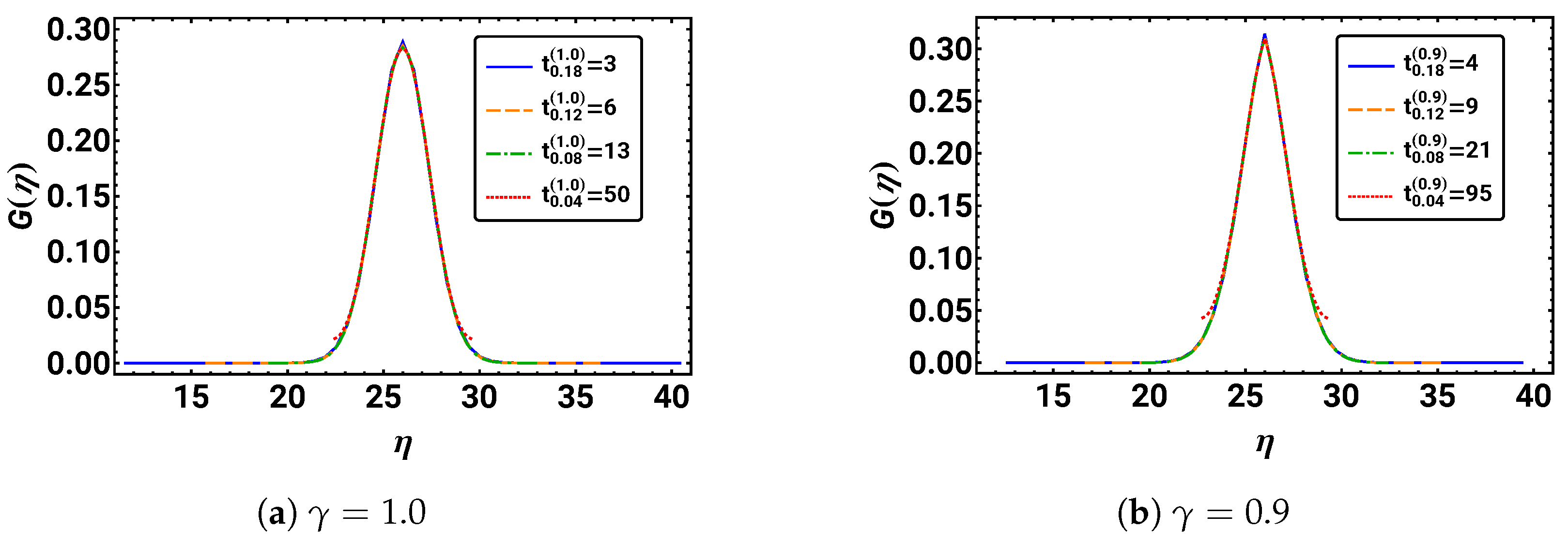
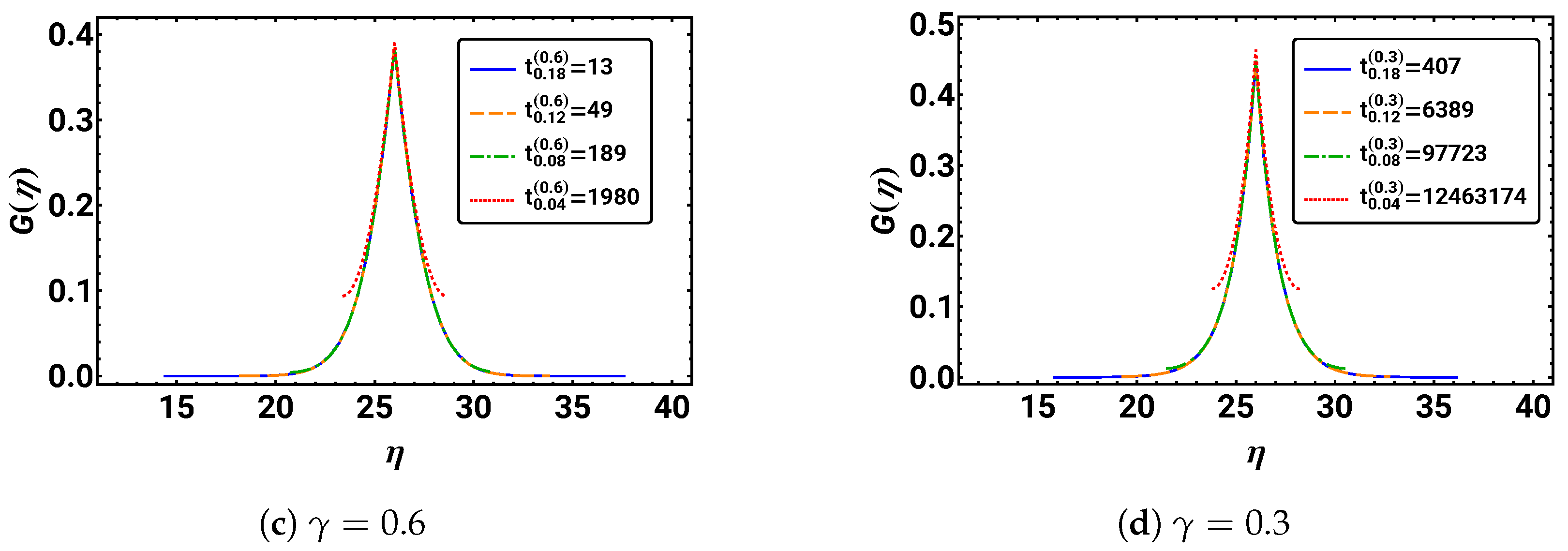
Create parametric plots of the probabilities $t^{\gamma /2}{P}_i\left(t\right)$ over $\eta (i,t)$ as a function of $0\le i\le 51$ for $\gamma =\{1.0,0.9,0.6,0.3\}$. For comparison, choose the same times as in Task 7 without $t_{0.02}^{\left(\gamma \right)}$.

The resulting plots are depicted in Figure 10. For different times t, the curves coincide very well, and the scaling property is indeed only valid in the short time regime. As soon as a considerable amount of probability reaches the boundaries, the tails of $\mathbf{G}\left(\eta \right)$ start to increase. Overall, the distributions show the expected scaling property for times at which they have not “felt” the boundaries.

Figure 10. The rescaled and normalized distributions $\mathbf{G}\left(\eta \right)$ for four different times is given over scaling variable $\eta$ for different values of $\gamma$.

While, for our discretized fractional master equation, the scaling features are approximate, we can show here for $\gamma =1$ that, for the continuous case, this scaling on an infinite domain is exact:

Theorem 2. 

Let $P(x,t)$ be the solution of the time-fractional diffusion equation

$$\begin{array}{cc}\hfill {\displaystyle \frac{{\partial }^{\gamma }}{\partial t^{\gamma }}}P(x,t)& =D_{\gamma }{\displaystyle \frac{{\partial }^2}{\partial x^2}}P(x,t),\hfill \end{array}$$

(60)

starting with a delta function, $P(x,0)=\delta \left(x\right)$ at time $t=0$. Let $\eta (x,t)=(x-x_0)/t^{\gamma /2}+x_0$ be a continuous rescaling of distances $(x-x_0)$ with time t. Then,

$$G(\eta ,t)=t^{\gamma /2}P(x(\eta ,t),t)$$

(61)

is time-independent.

For simplicity, we only consider the case where P becomes Gaussian (i.e., $\gamma =1$). The proof for a general $\gamma$ using H-function representations is beyond the scope of this article.

Proof. 

Solving $\eta (x,t)$ for x, one can express x as

$$\begin{array}{c}\hfill x=(\eta -x_0)t^{\gamma /2}+x_0.\end{array}$$

(62)

Utilizing the known probability density from Equation (3) for the $\gamma =1$ case, one can then explicitly check that the function $G(\eta ,t)=t^{\gamma /2}P(x(\eta ,t),t)$ is time-independent:

$$\begin{array}{cc}\hfill G(\eta ,t)& =t^{1/2}P(x(\eta ,t),t)\hfill \\ \hfill & =t^{1/2}{\displaystyle \frac{1}{2\sqrt{2\pi Dt}}}\exp \left(-{\displaystyle \frac{{\left((\eta -x_0)t^{1/2}\right)}^2}{4Dt}}\right)\hfill \\ \hfill & ={\displaystyle \frac{1}{2\sqrt{2\pi D}}}\exp \left(-{\displaystyle \frac{{(\eta -x_0)}^2}{4D}}\right).\hfill \end{array}$$

(63)

□

6. Summary

This paper presents a novel path to fractional calculus so readers may approach the subject in a less formal and more operational manner, making fractional diffusion equations in modern physical problems more easily addressed. Thus, the focus is on the physical context rather than the underlying mathematics.

For simplicity, we considered only the discrete one-dimensional time-fractional diffusion equation in a finite interval. We introduced the fractional derivative operator as an identity operator for a generalized exponential function (the Mittag–Leffler function $E_{\gamma }\left(t^{\gamma }\right)$) instead of discussing the underlying mathematical definition in detail. With this concept, we were able to solve the discretized time-fractional diffusion equation and formulate the solution in terms of the eigenvalues and eigenvectors of the system, where the eigenvalues represent the temporal modes of the time evolution of the probability distribution.

Using this solution, we investigated the time behavior of the time-fractional diffusion equation, representing anomalous subdiffusion and normal diffusion in a finite interval. We analyzed the spreading of the distributions via the mean square displacement $⟨{(i-i_0)}^2⟩$ of the probability distribution and discovered three different time regimes. We observed the power law behavior of the $⟨{(i-i_0)}^2⟩$, with an anomalous slow increase depending on the anomalous diffusion exponent $\gamma$ for short times, the stationary value independent of $\gamma$ due to the finite size of the interval, and the transition between both behaviors, being characterized by the temporal modes of the system. Additionally, we discussed the rescaling of the distributions for each $\gamma$ in the initial time regime by introducing a scaling variable $\eta (i,t)$, suggested by the initial power law behavior of $⟨{(i-i_0)}^2⟩$. Due to this scaling variable, all distributions for the different $\gamma$ values coalesce into one master curve for all (initial) times.

References

- Brown, R. A brief account of microscopical observations made in the months of June, July and August, 1827, on the particles contained in the pollen of plants; and on the general existence of active molecules in organic and inorganic bodies. Edinb. New Philos. J. 1828, 4, 358–371. [Google Scholar] [CrossRef]
- Jost, W. Grundlagen der Diffusionsprozesse. Angew. Chem. 1964, 76, 473–483. [Google Scholar] [CrossRef]
- Jungemann, C.; Zimmermann, C. DC, AC and noise simulation of organic semiconductor devices based on the master equation. In Proceedings of the 2014 International Conference on Simulation of Semiconductor Processes and Devices (SISPAD), Yokohama, Japan, 9–11 September 2014; pp. 137–140. [Google Scholar] [CrossRef]
- Stehr, V.; Fink, R.F.; Tafipolski, M.; Deible, C.; Engels, B. Comparison of different rate constant expressions for the prediction of charge and energy transport in oligoacenes. WIREs Comput. Mol. Sci. 2016, 6, 694–720. [Google Scholar] [CrossRef]
- Hoffmann, K.H.; Schön, J.C. Controlled dynamics on energy landscapes. Eur. Phys. J. B 2013, 86, 220. [Google Scholar] [CrossRef]
- Kunz, R.E.; Blaudeck, P.; Hoffmann, K.H.; Berry, R.S. Atomic clusters and nanoscale particles: From coarse-grained dynamics to optimized annealing schedules. J. Chem. Phys. 1998, 108, 2576–2582. [Google Scholar] [CrossRef]
- Gillespie, D.T. A rigorous derivation of the chemical master. Physica A 1992, 188, 404–425. [Google Scholar] [CrossRef]
- Gupta, A.; Rawlings, J.B. Comparison of parameter estimation methods in stochastic chemical kinetic models: Examples in systems biology. AIChE J. 2014, 60, 1253–1268. [Google Scholar] [CrossRef]
- Dorogovtsev, S.N.; Mendes, J.F.F.; Samukhin, A.N. Structure of growing networks with preferential linking. Phys. Rev. Lett. 2000, 85, 4633–4636. [Google Scholar] [CrossRef]
- Parthasarathy, P.R. A transient solution to an M/M/1 queue: A simple approach. Adv. Appl. Prob. 1987, 19, 997–998. [Google Scholar] [CrossRef]
- Grabowski, A.; Kosi, R.A. Epidemic spreading in a hierarchical social network. Phys. Rev. E 2004, 70, 031908. [Google Scholar] [CrossRef]
- Carslaw, H.S. Introduction to the Mathematical Theory of the Conduction of Heat in Solids, 2nd ed.; Macmillan and Co., Limited: London, UK, 1921. [Google Scholar]
- Gray, M.C. Particular Solutions of the Equation of Conduction of Heat in One Dimension. Proc. Edinb. Math. Soc. 1924, 43, 50–63. [Google Scholar] [CrossRef]
- Heins, A.E. Note on the Equation of Heat Conduction. Bull. Amer. Math. Soc. 1935, 41, 253–258. [Google Scholar] [CrossRef]
- Feller, W. An Introduction to Probability Theory and Its Applications, 2nd ed.; Wiley: New York, NY, USA, 1971. [Google Scholar]
- Vilk, O.; Aghion, E.; Avgar, R.; Beta, C.; Nagel, O.; Sabri, A.; Sarfati, R.; Schwartz, D.K.; Weiss, M.; Krapf, D.; et al. Unravelling the origins of anomalous diffusion: From molecules to migrating storks. Phys. Rev. Res. 2022, 4, 033055. [Google Scholar] [CrossRef]
- Havlin, S.; Ben-Avraham, D. Diffusion in Disordered Media. Adv. Phys. 1987, 36, 695–798. [Google Scholar] [CrossRef]
- Bunde, A.; Havlin, S. (Eds.) Fractals and Disordered Systems, 2nd ed.; Springer: Berlin/Heidelberg, Germany; New York, NY, USA, 1996. [Google Scholar]
- Appel, A.; Fleischer, F.; Kärger, J.; Fujara, F.; Siegel, S. NMR evidence of anomalous molecular diffusion due to structural confinement. Europhys. Lett. 1996, 34, 483–487. [Google Scholar] [CrossRef]
- Kärger, J.; Fleischer, G.; Roland, U. PFG NMR Studies of Anomalous Diffusion. In Diffusion in Condensed Matter; Kärger, J., Ed.; Vieweg-Verlag: Braunschweig, Germany, 1998; pp. 144–168. [Google Scholar]
- Franz, A.; Schulzky, C.; Seeger, S.; Hoffmann, K.H. Diffusion on Fractals—Efficient algorithms to compute the random walk dimension. In Fractal Geometry: Mathematical Methods, Algorithms, Applications; Blackledge, J.M., Evans, A.K., Turner, M.J., Eds.; IMA Conference Proceedings; Horwood Publishing Ltd.: Chichester, West Sussex, UK, 2002; pp. 52–67. [Google Scholar] [CrossRef]
- Franz, A.; Schulzky, C.; Seeger, S.; Hoffmann, K.H. An Efficient Implementation of the Exact Enumeration Method for Random Walks on Sierpinski Carpets. Fractals 2000, 8, 155–161. [Google Scholar] [CrossRef]
- Xue, C.; Huang, Y.; Zheng, X.; Hu, G. Hopping behavior mediates the anomlaous confined diffusion of nanoparticles in porous hydrogels. J. Phys. Chem. Lett. 2022, 13, 10610–10620. [Google Scholar] [CrossRef]
- Lui, Y.; Zheng, X.; Guan, D.; Jiang, X.; Hu, G. Heterogeneous Nanostructures cause anomalous diffusion in lipid monolayers. ACS Nano 2022, 16, 16054–16066. [Google Scholar] [CrossRef]
- Köpf, M.; Corinth, C.; Haferkamp, O.; Nonnenmacher, T.F. Anomalous Diffusion of Water in Biological Tissues. Biophys. J. 1996, 70, 2950–2958. [Google Scholar] [CrossRef]
- Tolić-Nørrelykke, I.M.; Munteanu, E.L.; Thon, G.; Oddershede, L.; Berg-Søorensen, K. Anomalous diffusion in living yeast cells. Phys. Rev. Lett. 2004, 93, 078102. [Google Scholar] [CrossRef]
- Gal, N.; Weihs, D. Experimental evidence of strong diffusion in living cells. Phys. Rev. E 2010, 81, 020903. [Google Scholar] [CrossRef]
- Schirmacher, W.; Perm, M.; Suck, J.B.; Heidemann, A. Anomalous Diffusion of Hydrogen in Amorphous Metals. Europhys. Lett. 1990, 13, 523–529. [Google Scholar] [CrossRef]
- Liu, S.; Bönig, L.; Detch, J.; Metiu, H. Submonolayer Growth with Repulsive Impurities: Island Density Scaling with Anomalous Diffusion. Phys. Rev. Lett. 1995, 74, 4495–4498. [Google Scholar] [CrossRef]
- Bénichou, O.; Coppey, M.; Moreau, M.; Suet, P.H.; Voituriez, R. Optimal Search Strategies for Hidden Targets. Phys. Rev. Lett. 2005, 94, 198101. [Google Scholar] [CrossRef] [PubMed]
- Bénichou, O.; Loverdo, C. Moreau, M.; Voituriez, R. Two-dimensional intermittent search processes: An alternative to Lévy flight strategies. Phys. Rev. E 2006, 74, 020102. [Google Scholar] [CrossRef]
- Shlesinger, M.F. Mathematical Physics—Search research. Nature 2006, 443, 281–282. [Google Scholar] [CrossRef] [PubMed]
- Cahoy, D.O.; Polito, F.; Phoha, V. Transient Behavior of Fractional Queues and Related Processes. Methodol. Comput. Appl. Probab. 2015, 17, 739–759. [Google Scholar] [CrossRef]
- Ascione, G.; Leonenko, N.; Pirozzi, E. Fractional Queues with Catastrophes and their Transient Behaviour. Mathematics 2018, 6, 159. [Google Scholar] [CrossRef]
- Souza, M.d.O.; Rodriguez, P.M. On a fractional queueing model with catastrophes. Appl. Math. Comp. 2021, 410, 126468. [Google Scholar] [CrossRef]
- Saxena, R.K.; Mathai, A.M.; Haubold, H.J. Computational Solutions of Distributed Order Reaction-Diffusion Systems Associated with Riemann-Liouville Derivatives. Axioms 2015, 4, 120–133. [Google Scholar] [CrossRef]
- Hoffmann, K.H.; Essex, C.; Schulzky, C. Fractional Diffusion and Entropy Production. J. Non-Equilib. Thermodyn. 1998, 23, 166–175. [Google Scholar] [CrossRef]
- Metzler, R.; Klafter, J. The random walk’s guide to anomalous diffusion: A fractional dynamics approach. Phys. Rep. 2000, 339, 1–77. [Google Scholar] [CrossRef]
- Klages, R.; Günther, R.; Sokolov, I.M. (Eds.) Anomalous Transport—Foundations and Applications; Wiley-VCH: Weinheim, Germany, 2008. [Google Scholar]
- Paradisi, P. Fractional calculus in statistical physics: The case of time fractional diffusion equation. Commun. Appl. Ind. Math. 2014, 6, 530. [Google Scholar] [CrossRef]
- Podlubny, I. Fractional Differential Equations—An Introduction to Fractional Derivatives, Fractional Differential Equations, to Methods of their Solution and some of their Applications; Mathematics in Science and Engineering; Academic Press: San Diego, CA, USA, 1999; Volume 198. [Google Scholar]
- Arqub, O.A.; El-Ajou, A.; Zhour, Z.A.; Momani, S. Multiple Solutions of Nonlinear Boundary Value Problems of Fractional Order: A New Analytic Iterative Technique. Entropy 2014, 16, 471–493. [Google Scholar] [CrossRef]
- Ahmad, J.; Mohyud-Din, S.T.; Srivastave, H.M.; Yang, X.J. Analytic solutions of the Helmholtz and Laplace equations by using local fractional derivative operators. Waves Wavelets Fractals Adv. Anal. 2015, 1, 22–26. [Google Scholar] [CrossRef]
- Povstenko, Y. Linear Fractional Diffusion-Wave Equation for Scientists and Engineers, 1st ed.; Birkhäuser: Basel, Switzerland, 2015. [Google Scholar] [CrossRef]
- Manapany, A.; Fumeron, S.; Henkel, M. Fractional diffusion equations interpolate between damping and waves. J. Phys. A Math. Gen. 2024, 57, 355202. [Google Scholar] [CrossRef]
- Caputo, M. Linear Models of Dissipation whose Q is almost Frequency Independent-II. Geophys. J. R. Astron. Soc. 1967, 13, 529–539. [Google Scholar] [CrossRef]
- Davison, M.; Essex, C. Fractional Differential Equations and Initial Value Problems. Math. Sci. 1998, 23, 108–116. [Google Scholar]
- Rogosin, S. The Role of the Mittag-Leffler Function in Fractional Modeling. Mathematics 2015, 3, 368–381. [Google Scholar] [CrossRef]
- Rogosin, S.V.; Giraldi, F.; Mainardi, F. On differentiation with respect to parameters of the functions of the Mittag-Leffler type. Integral Transform. Spec. Func. 2024, 1–13. [Google Scholar] [CrossRef]
- Mainardi, F. On some properties of the Mittag-Leffler function Eα(−tα), completely monotone for t > 0 with 0 < α < 1. Discete Cont. Dyn.-B 2014, 19, 2267–2278. [Google Scholar] [CrossRef]
- Zwillinger, D. Handbook of Differential Equations, 3rd ed.; Academic Press: San Diego, CA, USA, 2007. [Google Scholar]
- Das, S. Solution of Extraordinary Differential Equations with Physical Reasoning by Obtaining Modal Reation Series. Modell. Simul. Eng. 2010, 2010, 739675. [Google Scholar] [CrossRef]
- Hoffmann, K.H.; Kulmus, K.; Essex, C.; Prehl, J. Between Waves and Diffusion: Paradoxical Entropy Production in an Exceptional Regime. Entropy 2018, 20, 881. [Google Scholar] [CrossRef] [PubMed]
- Kulmus, K.; Essex, C.; Prehl, J.; Hoffmann, K.H. The entropy production paradox for fractional master equations. Physica A 2019, 525, 1370–1378. [Google Scholar] [CrossRef]
Disclaimer/Publisher’s Note: The statements, opinions and data contained in all publications are solely those of the individual author(s) and contributor(s) and not of MDPI and/or the editor(s). MDPI and/or the editor(s) disclaim responsibility for any injury to people or property resulting from any ideas, methods, instructions or products referred to in the content. |
© 2025 by the authors. Licensee MDPI, Basel, Switzerland. This article is an open access article distributed under the terms and conditions of the Creative Commons Attribution (CC BY) license (https://creativecommons.org/licenses/by/4.0/).