Abstract
The Mixed No-Idle Permutation Flow Shop Scheduling Problem (MNPFSSP) represents a specific case within regular flow scheduling problems. In this problem, some machines allow idle times between consecutive jobs or operations while other machines do not. Traditionally, the MNPFSSP has been addressed using the metaheuristics and exact methods. This work proposes an Evolutionary Strategy Based on the Generalized Mallows Model (ES-GMM) to solve the issue. Additionally, its advanced version, ES-GMMc, is developed, incorporating operating conditions to improve execution times without compromising solution quality. The proposed approaches are compared with algorithms previously used for the problem under study. Statistical tests of the experimental results show that the ES-GMMc achieved reductions in execution time, especially standing out in large instances, where the shortest computing times were obtained in 23 of 30 instances, without affecting the quality of the solutions.
1. Introduction
The Mixed No-Idle Permutation Flow Shop Scheduling Problem (MNPFSSP) is a mixed-integer scheduling problem in which both types of machines with idle time and no idle time are allowed, depicting a real-world scenario. This problem was first raised by Pan and Ruiz in 2014 and cataloged as NP-hard. Currently, the problem is solved by considering the only objective to be the maximum completion time or makespan, denoted as , although new variants of the problem have emerged that include additional features and other target functions [1,2].
The MNPFSSP is challenging not only due to the combination of constraints imposed on machines, with and without idleness, but also because it guarantees the coexistence of both types of machines. It makes it more difficult and expensive to select feasible solutions to minimize the objective function.
In the state-of-the-art Iterated Greedy metaheuristics [3], exact methods, such as Benders Decomposition (BD), branch-and-cut (BC), and Automated Benders Decomposition (ABD), as well as metaheuristics [4], such as the Iterated Greedy algorithm (IGA) and Referenced Local Search (RLS), have been used to solve the aforementioned problem. In this study, the proposed algorithm is compared against the metaheuristics and some exact methods that decompose the MNPFSSP.
The decomposition methods are applied to problems that allow identifying structures in the constraints of linear programming problems. An example is the mixed-integer mathematical programming (MILP) problems, where their difficulty lies in the fact that they have some variables of an integer nature, causing the convexity property of the feasible region to be lost, making it difficult to solve the problem [5]. In these cases, the aim is to break down the original problem into subproblems that are more easily solvable than the original problem, taking advantage of their iterative solution. In particular, the Benders Decomposition Method (BD) identifies complicating variables as those that, when set as parameters, make the search process easier, breaking down the problem into two simpler ones, which are called the master problem and the subproblem [4].
In this scheme, the solution to the problem is derived by finding partial solutions to the master problem and subproblem using a feedback scheme. Convergence to the solution of the original problem is sought through the information on the dual problems associated with the subproblem, i.e., the master problem solves the complicating variables, and the subproblem is solved by setting such variables. Furthermore, the subproblem gives feedback to the master problem through the solution of the dual problem. The goal is to optimize a feasible region by increasing constraints (called cuts) to approximate the optimal solution [4,5]. The above description assumes that the subproblem is feasible and bound for any master problem, but this condition is not always satisfied; thus, the method is modified by constructing the feasibility cut. If the subproblem is feasible, its solution generates optimality cuts for the master problem. BD has the advantage of having a feasible solution: even if convergence is not achieved, it generates a quasi-optimal solution [6].
The branch-and-cut (BC) method is a combination of the cutting plane algorithm with the branch-and-bound method. A cut plane is a linear constraint that is added to the linear programming (LP) relaxation at any node in the search tree. Given an integer problem (IP), the BC method searches the feasible region by building a binary search tree, solving for the LP relaxation of the IP input, and then adding any number of cut planes [7].
Contrarily, the Estimation of Distribution Algorithms (EDAs) belong to the evolutionary computation field, specifically among the stochastic algorithms that simulate a natural evolution, known as evolutionary algorithms, which depend on parameters such as crossover and mutation operators, crossover and mutation probabilities, population size, number of generations, etc. Establishing appropriate values for these parameters has become an optimization problem, which has motivated the emergence of EDAs. They were first introduced in 1996 by Mühlenbein [8].
EDAs have been applied to solve combinatorial optimization problems [9,10,11], achieving competitive performance. Therefore, we justify their application for the MNPFSSP.
EDAs mainly replace crossover and mutation operators by estimating and sampling a probability distribution commonly learned from individuals (solution vectors) of the previous generation. An attempt is made to explicitly find correlations between the variables, i.e., the interactions between the variables (the genes of the individuals). Such interactions are expressed through the probability distribution associated with the selected individuals in each generation [12]. This is one of the most complicated features of the EDAs, i.e., estimating the probabilistic model that represents the interactions between the variables of the selected individuals. In addition, other factors such as individual representation and objective function are decisive factors in the process [13].
This study presents an evolutionary strategy implemented using the ES-GMM algorithm. The proposal is inspired by an EDA that uses the Generalized Mallows Distribution (GMM). The ES-GMM focuses on a practical proposal for estimating the parameters of the GMM and the operating conditions. The ES-GMM performance is compared against the exact methods applied in [3] to solve the MNPFSSP.
The article is organized as follows: Section 2 presents the state of the art, including an overview of EDAs based on the Mallows Model. Section 3 provides the background, including a description of the MNPFSSP, the EDA based on the Mallows Model, and the GMM. Section 4 describes the proposed ES-GMM algorithm, including its advanced version ES-GMMc. Section 5 presents experimental development, while Section 6 presents the results and statistical analysis, comparing the performance of ES-GMM and ES-GMMc with BC, ABD, IGA, and RLS. Section 7 provides a discussion of the main findings, highlighting the contributions, practical implications, and comparative advantages of the proposed approach. Finally, Section 8 presents the conclusions and future research.
2. State of the Art
In recent years, EDAs have been proposed to solve problems similar to the MNPFSSP, such as the PFSSP [11] and NPFSSP [12]. These approaches adapt from discrete and continuous domains to the permutation’s domain. Ceberio et al. [14,15] proposed the application of EDAs in permutation spaces and suggested probabilistic models such as those based on marginal, the Plackett–Luce and Mallows Models. Although the Mallows Model has shown competitive results, there has been a recognized need for a deeper study, particularly regarding parameter estimation [10,16].
Ceberio et al. [14] introduced a marginal -order model that considers interactions among all problem variables through a matrix reflecting the joint probability of an index being in a specific position. This model, with a memory cost of is practical only for small values of (size of the marginal matrix) and (problem size). The authors observed the necessity of modeling probability distributions over permutations and proposed to use the Mallows Model for this purpose [17], which is defined by two parameters: a central permutation (estimated by sampling and averaging permutations) and a spread parameter (defined via Maximum Likelihood Method (MLE) and calculated numerically), to balance the exploration and exploitation of the solution space. Specifically, with small values of the probability assigned to was also small (exploration), but it increased rapidly once surpassed a certain threshold (exploitation).
Although the EDA working with the Mallows Model outperformed other algorithms for large instances of the Flow Shop Scheduling Problem (FSSP), despite the numerical challenge posed by the estimation of its parameters, a lack of control of the algorithm was observed, and the necessity for a better understanding of the spread parameter was indicated [15].
Ceberio et al. [3] detailed a generalization of the EDA working with the Mallows Model, facing similar instability issues, as previously observed. Empirical values and an upper bound for were defined to balance exploration and exploitation and avoid premature convergence [3]. To estimate the central permutation , the Maximum Likelihood Method was formulated, leading to being given by the permutation that minimizes the sum of Kendall distances of the sample. This problem is known as the Kemeny Rank Aggregation Problem and is recognized as NP-hard. An alternative to estimating the central permutation was performing an exhaustive analysis to find an exact or approximate solution for the central permutation, and it was concluded that the Borda algorithm offers a balance between computation time and accuracy, providing an unbiased estimator of the Kemeny problem solution [18]. Some studies have focused on improving the quality of by applying mutation methods [19], heuristics or metaheuristics [20], and Pareto front approaches [21].
Recently, several studies have explored the use of different distance metrics, such as Cayley and Ulam, for the GMM [3,13,18,22,23]. These advancements highlight the effectiveness of the Mallows Model in permutation optimization and suggest that implementation within an EDA framework should be promising for the MNPFSSP.
Despite the performance of previous implementations, the literature reveals a persistent challenge in systematically estimating GMM parameters. Studies continue to rely on empirical methods for parameter estimation, underscoring the need for improved precision in this process.
3. Background
3.1. The MNPFSSP
The MNPFSSP, denoted as , belongs to the family of pure regular flow scheduling problems. It is a general case of the NPFSSP where some machines allow idle times while other machines do not: this problem is considered NP-hard. The objective is to find the optimal job sequence that minimizes the maximum completion time (makespan) [3].
The NPFSSP differs from the basic Permutation Flow Shop Scheduling Problem (PFSSP) because there is no idle time allowed between two consecutive jobs on the machines. This feature is established in the PFSSP by the condition that the completion time of a job on the machine is greater than or equal to the completion time of the previous job on the same machine plus its processing time. Meanwhile, in the case of NPFSSP, it is enforced as equality. Considering these two conditions, the mathematical model of the MNPFSSP can be modeled as a mixed-integer linear problem, where the objective function consists of the minimization of the makespan, i.e., the completion time at which the job that occupies the last position of the sequence on the last machine ends [3]. This is defined by the next equation.
It is subject to the following:
where
- is the completion time of work at position on machine .
- indicates whether a job occupies a position in the sequence, taking the value 1 or 0.
- is the processing time for job on machine .
- is a no-idle machines subset of .
The constraints (2) and (3) enforce that each job occupies a position in the permutation and that each position in any permutation is occupied by a job. Constraint (4) controls the completion time of the first job in the permutation. Constraint (5) imposes that the completion times of jobs on the second and subsequent machines are larger than the completion times of the previous tasks of the same job on previous machines plus its processing time, effectively avoiding the overlap of tasks from the same job position. Furthermore, the constraint (6) seeks to respect the existence or inexistence of inactive times [3,4].
Solution Representation
To generate a schedule for the MNPFSSP, a permutation-based representation is used in this study. In this representation, each element of the permutation, represented by an integer, corresponds to a specific job. The order of elements in the permutation defines the sequence in which the jobs will be processed in the machines from the production line. The solutions can be represented using Gantt charts. In Figure 1, we show the Gantt charts for the PFSSP, NPFSSP, and MNPFSSP, where represents the machines and the jobs in the sequence. We can notice the existence of no-idle and idle machines according to the characteristics of each problem.
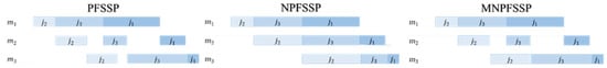
Figure 1.
Gantt charts for the PFSSP, NPFSSP and MNPFSSP solutions.
3.2. EDAs Coupled with the GMM
The EDAs were first introduced in the field of evolution by Mühlenbein and Paaß [8], constituting a new tool in the field of evolutionary computation. They can be considered as a generalization of Genetic Algorithms (GAs), where the reproduction operators (crossover and mutation) are replaced by the estimation and sampling of the probability distribution of selected individuals [8].
The EDA constructs a probability distribution of the most promising solutions by leveraging the interrelationships between problem features. The distribution model is used to generate new individuals. The process is iterative, until a stopping criterion is met, and it returns the best-found solution.
Due to the need to solve permutation combinatorial problems, which are highly relevant in real-world situations in the industry, the EDA researchers have focused on developing new strategies to solve permutation-based problems. The Generalized Mallows Model on Estimation of Distribution Algorithm (GMMEDA) arises from a previous idea and has been applied to scheduling problems such as the PFSSP [3].
3.2.1. The GMM
The Mallows Model is a distance-based exponential probability model over permutation spaces that is based on the distance , which consists of counting the number of inversions necessary to order one permutation compared to another . From this metric, the distribution is defined by Equation (9), with the parameter’s central permutation and the spread parameter .
where is a normalization constant. When assigns equal probability to every permutation, the larger the value of , the greater the probability assigned to . Thus, each permutation is assigned a probability that decays exponentially with respect to its distance from the central permutation [3].
The GM model was proposed as an extension of the Mallows Model [3]. This extension requires that the distance used can be decomposed into terms, such that the distance between permutations is expressed as , where is the number of positions with smaller values to the right of . When using the Kendall distance, the term is denoted by and is defined as , and it ranges from to for . Then, Equation (9) is rewritten as follows:
Considering as independent variables, the probability distribution for the variables under the GM model is given by
To introduce the GM model into an EDA concept, it is necessary to estimate its parameters and . These are estimated using the principle of Maximum Likelihood Estimation (MLE). MLE starts from a sample of permutations where parameters and maximize the likelihood function shown in Equation (12).
where
3.2.2. Position Parameter
Maximizing the log-likelihood with respect to is equivalent to minimizing , and the central permutation is the minimum of the sum of the Kendall distances of a sample of permutations. Such estimation itself constitutes a problem classified as NP-hard, known as the Kemeny Rank Aggregation Problem [4]. In recent studies, the Borda algorithm has been used to compute the central permutation in the GMM, which has shown a good balance between time and quality of the solution [3].
3.2.3. Spread Parameter
The spread parameter for the GM model is estimated by using the likelihood function (12). For this purpose, the central permutation is taken, and the estimation is obtained by solving (14), which does not have a closed-form expression, but can be solved numerically using standard iterative algorithms for convex optimization. The Newton–Raphson method has been used for estimating the spread parameter in the literature [4].
The pseudocode of the algorithm based on the EDA coupled with the GMM is presented in Algorithm 1, and this follows the procedure adopted in the state of the art. This approach is known in the literature as the GMEDA.
| Algorithm 1: EDAs coupled with the GMM |
| . . for each individual according [24]. . . . . End While . |
4. Evolutionary Strategy Based on the Generalized Mallows Model (ES-GMM)
The Differential Evolution Estimation Distribution Algorithm (DE-EDA) [4], the hybrid Estimation Distribution Ant Colony Search Algorithm (EDA-ACS) [5], and the Random Key-EDA [6] have been used for solving the Permutation Flow Shop Scheduling Problem (PFSP). In the case of PFSP, an EDA-GMM algorithm based on the ranking of distances has been applied [4]. This contribution was used as a reference to adapt and propose the version ES-GMM to solve the MNPFSSP.
In the proposed evolutionary strategy, each individual in the population is represented as a job permutation. This representation defines the sequence in which jobs are processed across machines. The population consists of many permutations, each evaluated based on its makespan, computed according to the methodology in [24].
To apply the GMM probabilistic model in our evolutionary strategy, the algorithm estimates the central and the spread parameters and . selects the individual with the smallest makespan from the selected population, and the spread parameter is proposed to be the inverse of the Kendall distances to the central parameter, according to Equation (15). These parameters are used to generate the offspring. This process is repeated until the predefined maximum generation is reached. The structure of the algorithm is depicted in Figure 2.
Figure 2.
Flowchart of ES-GMM algorithm.
4.1. Hyperparameters of Evolutionary Strategy
For the design of the proposed evolutionary strategy, the values of the hyperparameters were selected based on an exhaustive review of the literature and systematic experimentation. These hyperparameters are maximum number of generations, population size, selection percentage, and sampling percentage. The justification for each one is detailed below.
4.1.1. Maximum Number of Generations
The maximum number of generations was set at , in accordance with values reported in previous studies for similar problems [3]. According to the literature, this value ensures an adequate balance between computing time and the search space exploration capacity, allowing convergence towards high-quality solutions.
4.1.2. Population Size
The population size
was defined based on the number of jobs (n) in each instance of the MNPFSSP. During the experimentation, different configurations were evaluated (
, among others), and it was observed that the N = 10n ratio offered better performance, maintaining population diversity throughout the optimization process, showing better adaptation to the complexity of the problem and producing higher-quality solutions.
4.1.3. Selection Rate
Three selection rate settings were tested, i.e., and . Experimental results indicated that a rate of was the most suitable for all instances, as it improved both solution quality and time efficiency. For small instances, this rate yielded significantly better solutions, while for large instances, it proved to be the most efficient setting in terms of runtime.
4.1.4. Sampling Rate
The sampling rate defines the proportion of individuals retained from the previous population. The sampling rates of
and were tested, using Relative Percentage Deviation (RPD) as the performance metric. Experimental analysis showed that a rate of
yielded the best results, with RPD values of
for small instances and
for large instances. This percentage not only outperformed the most common configurations in the literature but also ensured consistent and high-quality solutions.
4.2. Estimation of Proposed Spread Parameter
We propose estimating the spread parameter based on the inverse relationship between the Kendall distance and the parameter value . This is proposed due to the difficulty of finding the spread value from Equation (14), as in the state of the art. Therefore, a practical proposal such as Equation (15) is proposed. When the average Kendall distance is large, it indicates greater diversity among the permutations, promoting exploration. Conversely, when is small, the sample of permutations converges toward the central permutation, favoring exploitation. Figure 3 illustrates the behavior of the with respect to the values assigned for , for both Equation (14) and the proposed Equation (15). The proposed relation achieves higher values for the , with respect to , allowing for greater exploration and improving the diversity of solutions. Regarding Equation (15), it is not necessary to perform additional calculations.
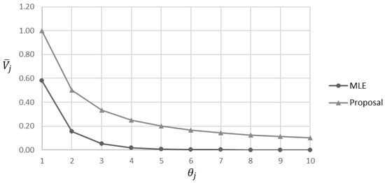
Figure 3.
Behavior of the average Kendall distance as a function of the spread parameter for the MLE and the proposed approach.
4.3. Operating Conditions of ES-GMMc
To establish the minimum number of generations for the algorithm to generate satisfactory solutions, an experimental analysis was carried out on samples of small and large instances for the MNPFSSP. Figure 4 and Figure 5 show the behavior of the algorithm’s makespan over 100 generations in small and large instances, respectively. To propose a reference value for , i.e., the smallest number of generations necessary so that the search process of the algorithm does not stop before approaching its convergence value, an experiment was carried out using a sample of the benchmark defined by Bektas, Hamzadayi, and Ruiz (2020) [4], which was built on the instance I_3_500_50_1, available at http://soa.iti.es/problem-instances, accessed on 1 January 2022. This benchmark classifies instances into two categories, i.e., small and large, according to the number of jobs. For the small instance category, the selected identifiers were , while for the large instances, the selected identifiers were. Table 1 and Table 2 present the ID, the number of jobs and the number of machines for the small and large instances, respectively.
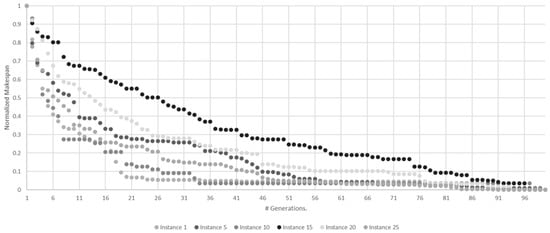
Figure 4.
Evolution of normalized average makespan across generations for small instances.
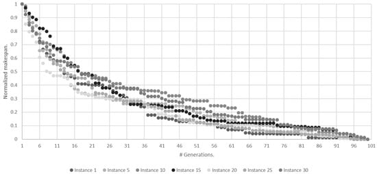
Figure 5.
Evolution of normalized average makespan across generations for large instances.

Table 1.
Characteristics of the small instances group [3].
Table 2.
Characteristics of the large instances group [3].
The graphs in Figure 4 and Figure 5 show the normalized average makespan of 30 experiments of 100 generations each for small and large instances, respectively.
From the observed behavior, the value was obtained, which represents the minimum generation number in which the algorithm converges in each instance. This value represents the generation where no more changes are observed in the makespan per instance. Table 3 shows the values, the average values, and their standard deviation for small and large instances.
Table 3.
Minimum number of generations where the algorithm converges. The results were experimentally obtained for small and large instances.
Based on the previous information, was defined as follows:
This was established as the minimum number of generations required before applying an algorithm stop condition.
Stopping Condition
The stopping criterion considers two key aspects: (1) reaching the minimum number of generations to avoid local minima and (2) confirming that the best makespan no longer improves after next generations.
Based on the calculated b value, a stopping condition was established to reduce the algorithm execution time. According to the flowchart in Figure 6, the stopping condition is defined as follows:
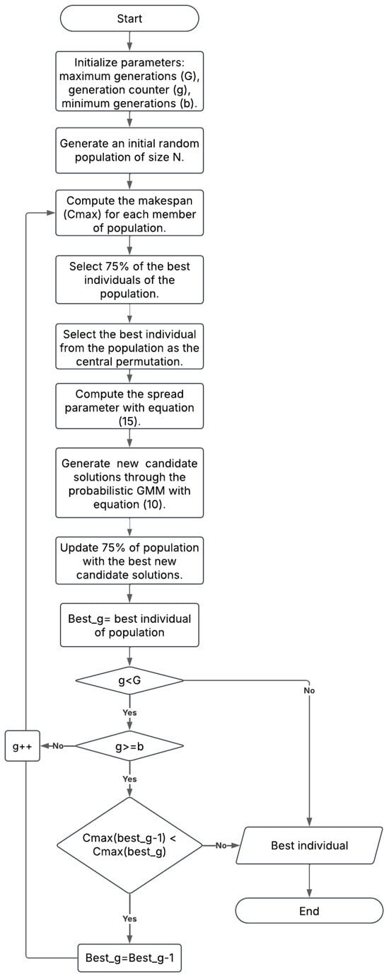
Figure 6.
Flowchart of ES-GMMc algorithm.
- The algorithm continues running for at least b generations, regardless of whether the makespan remains constant.
- After b generations, if the makespan of the best individual remains constant, the algorithm stops.
This stopping criterion ensures that the algorithm has enough time to explore solutions during the first generations while allowing it to terminate early once it is clear that no further significant improvements are achievable. This approach accelerates the convergence process and reduces the execution time when the algorithm has reached a local or global optimum.
Figure 6 presents the flowchart of the ES-GMMc algorithm, highlighting the incorporation of a stopping criterion. The flowchart illustrates each stage of the algorithm, from the initial population generation to the selection of the best individuals and the updating of the parameters of the Mallows Distribution. In addition, the stopping conditions are detailed, where the algorithm verifies whether it has reached the threshold of generations or whether the makespan of the best individual has stabilized, in which case the execution is interrupted early.
5. Experimental Development
The proposed algorithm was executed in two versions with the same hyperparameters, without the stop condition (ES-GMM) and with the stop condition (ES-GMMc). To evaluate the results, they were compared to those of the exact methods (BC, BD, and ABD) reported in the study by Bektas, Hamzadayi, and Ruiz [4]. Since the results obtained by the BD method were not fully reported in the literature, they were re-evaluated experimentally. Additionally, the proposed algorithms were compared with the metaheuristics IGA and RLS.
Experiments were conducted on a desktop computer equipped with an Intel® Core™ i9-9900K CPU @ 3.60 GHz and 32 GB RAM. The exact methods were solved using the Cplex Studio IDE 12.9.0, while the metaheuristics were implemented in Java using the IDEA Community Edition 2018.
5.1. Instance Generation
The experimental instances were derived from a benchmark instance with 500 jobs and 50 machines, available at http://soa.iti.es. From this, the following subsets were generated: 27 small instances, with and , and 30 large instances, with and .
5.2. Methodology
To compare makespan results with those reported in the state of the art, each algorithm was executed 30 experiments for each instance, and the minimum makespan obtained was recorded.
For the BD method, a limit time of 7200 s was imposed, consistent with the methodology in [1]. The reported time corresponds to the duration required to achieve the optimal solution or the best solution within the time limit. For the ES-GMM and ES-GMMc algorithms, the average execution time over the 30 experiments was reported.
This setup ensures a fair comparison of performance, focusing on both solution quality (makespan) and computational efficiency (execution time).
6. Results
This section presents the results obtained in terms of makespan and execution time for both small and large instances. The analysis focuses on comparing the performance of the different algorithms, evaluating their efficiency in terms of solution quality (makespan) and computational cost (execution time), incorporating a detailed statistic by evaluation and determining whether the observed differences are significant. The primary objective is to identify algorithms that achieve an appropriate balance between solution quality and computational cost, supported by statistical analysis.
6.1. Small Instances
6.1.1. Makespan Results
Figure 7 presents a comparative analysis of the makespan obtained by all the algorithms for small instances. Boxplots were used to visualize the distribution of results and evaluate the performance of each approach. It was observed that the ES-GMMc algorithm demonstrates competitive performance in terms of makespan, maintaining values close to the median of the most effective methods compared to the other approaches.
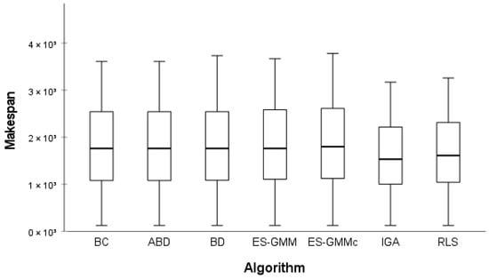
Figure 7.
Makespan obtained by algorithms for small instances.
6.1.2. Statistical Analysis of Makespan
To formally assess whether there are statistically significant differences between algorithms regarding the makespan, normality and homogeneity tests were first applied with a significance level of . The Shapiro–Wilk test confirmed that the makespan data follow a normal distribution , and the Levene test confirmed the homogeneity of variances . Therefore, an ANOVA test was applied with the null hypothesis that all algorithms exhibit equivalent performance.
The ANOVA test returned a -value of , indicating that there are no statistically significant differences between the makespan performance in small instances. Although ES-GMMc shows competitive values in absolute terms, this difference is not statistically significant.
6.1.3. Execution Time Results
The execution times of the different algorithms for small instances are shown in Figure 8. It was observed that the BD algorithm exhibits a high variability, with significantly higher outlier values compared to the rest of the methods. Due to this variability, nine outlier extreme values were excluded from the BD algorithm to provide a clearer view of the performance of the remaining algorithms.
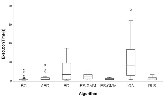
Figure 8.
Execution times obtained by algorithms for small instances. represents moderate outliers, and represents extreme outliers.
In Figure 8, the IGA presents the highest dispersion and presence of outliers, indicating that its execution time is less predictable and, in some cases, considerably higher than that of the rest of the algorithms.
In contrast, the ES-GMMc algorithm maintains low and relatively stable execution times, without any outliers, reaffirming its computational efficiency. BC, ABD, and ES-GMM present similar execution times, although BC and ABD show a larger number of outliers, indicating that their performance may vary depending on the instance being solved. The RLS algorithm stands out for its low and consistent execution times, suggesting that it is an efficient option in terms of computational cost.
The combined analysis of makespan and execution time suggests that the ES-GMMc achieves a favorable balance between solution quality and computational efficiency, positioning it as a strong candidate for solving small instances. Although the IGA achieves competitive makespan values, its higher computational cost makes it less attractive for time-constrained environments. Finally, RLS emerges as an efficient option in terms of computational cost, although there is no significant difference in the quality of the solution, compared to the rest of the algorithms.
6.1.4. Statistical Analysis of Execution Times
Normality and homogeneity tests (Shapiro–Wilk and Levene) were applied with a significance level of . Both tests indicated that execution times do not follow a normal distribution (see Table 4); thus, a non-parametric Friedman test was applied to evaluate differences between algorithms. The Friedman test calculated a -value of , indicating significant differences in execution times.
Table 4.
Statistical test results of the execution times for small instances.
The average ranks of Friedman (see Table 4) show that the BC method and the ES-GMMc achieve the shortest execution times, with the IGA being the least efficient. To further validate these findings, a Wilcoxon post hoc test was performed comparing the four best-ranked algorithms (see Table 5).
Table 5.
Results of Wilcoxon post hoc test of the execution times for small instances.
The post hoc analysis (see Table 5) confirms that the BC method is better than the ES-GMMc, ABD, and RLS, which achieve statistically similar execution times.
6.2. Large Instances
6.2.1. Makespan Results
Figure 9 presents the makespan performance of the algorithms for large instances. In general, all algorithms present a similar range of values, with medians close to each other. However, slight differences were observed. In particular, the IGA presents a slightly lower median makespan, indicating that it marginally outperforms the other approaches in terms of solution quality.
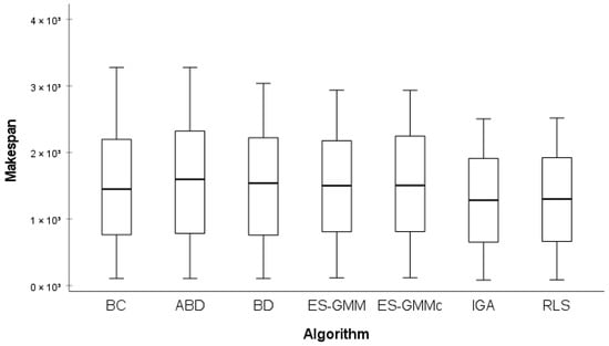
Figure 9.
Makespan obtained by different algorithms for large instances.
Contrarily, algorithms such as BC, ABD, and BD show a wider range, indicating higher variability in their performance across different instances. The ES-GMMc algorithm maintains stable performance, with a competitive median and lower dispersion compared with BC and ABD. Similarly, RLS shows consistent behavior, with median and variability levels comparable to IGA, highlighting its ability to maintain stable solution quality across larger instances.
6.2.2. Statistical Analysis of Makespan
The Shapiro–Wilk and Levene tests were applied with a significance level of . The Shapiro–Wilk (-value: ) and Levene tests (-value: ) confirmed the normality and homogeneity of variances, justifying the use of an ANOVA test. The ANOVA test returned a -value of , indicating that there are no statistically significant differences between algorithms regarding makespan in large instances.
This result implies that, although the IGA achieves the best makespan values in absolute terms, these differences are not statistically significant and therefore cannot be used as conclusive evidence of its superiority in terms of solution quality.
6.2.3. Execution Time Results
The execution times for large instances are presented in Figure 10. As observed in small instances, the IGA presents an extremely high outlier, which implies that, in at least one instance, its execution time was significantly longer than the others. To provide a clearer view of the remaining algorithms, two extreme outliers were excluded from the IGA.
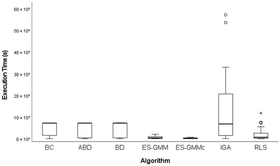
Figure 10.
Execution times obtained by different algorithms for large instances. represents moderate outliers, and represents extreme outliers.
In this revised comparison, the ES-GMMc and ES-GMM stand out as the algorithms with the shortest execution times. Notably, the ES-GMMc reduced the execution time in 23 out of 30 instances. Both approaches not only achieved low execution times but also demonstrated very controlled variability, with compact boxes and short whiskers, indicating consistent performance for different instances.
In contrast, algorithms such as ABD, BC, and BD presented considerably longer execution times. Their boxes were more elongated, which suggested that these methods were more sensitive to the specific characteristics of each instance, causing highly variable resolution times.
The RLS algorithm showed relatively low execution times compared to the exact approaches (ABD, BC, and BD), but higher than those observed in the ES-GMM and ES-GMMc.
The combined analysis of makespan and execution times for large instances reinforces the conclusion that the ES-GMMc achieves a favorable balance between solution quality and computational efficiency, positioning it as a robust and competitive approach for solving larger problem instances. Although the IGA achieves competitive makespan values, its high computational cost limits its suitability for time-sensitive scenarios. Finally, RLS offers a balanced alternative, combining moderate computational cost with relatively stable solution quality, although it does not reach the same level of performance as the ES-GMMc.
6.2.4. Statistical Analysis of Execution Times
The Shapiro–Wilk and Levene tests confirmed that the execution times do not follow a normal distribution , necessitating the use of the non-parametric Friedman test. The Friedman test calculated a -value of , indicating significant differences between algorithms. Table 6 presents the average ranges showing that the ES-GMMc achieves the best (shortest) execution times, followed closely by the ES-GMM and RLS, while the IGA exhibits the longest execution times.
Table 6.
Friedman test of execution times for large instances.
A Wilcoxon post hoc test was applied to confirm the differences between the top four algorithms. The test confirmed that the ES-GMMc execution time is significantly lower than its competitors , supporting the conclusion that the ES-GMMc is the most computationally efficient algorithm for large instances.
7. Discussion
This section discusses the performance of the proposals, mostly the key factors that contribute to the performance of the algorithm, with special emphasis on the stopping criterion, which allows an improvement in computational efficiency without compromising the quality of the solution. The strengths and weaknesses of the proposed method are identified and compared with those of the existing programming techniques. Finally, the practical implications of these findings for real-world production environments are examined, highlighting the potential advantages and applications of the proposed approach.
7.1. Stopping Criterion and Computational Efficiency
One of the key contributions of the ES-GMMc, the advanced version of the ES-GMM, is the incorporation of a stopping criterion. This criterion, experimentally defined and based on an evolution analysis of the normalized makespan through the generations, allows the algorithm to terminate once the convergence patterns are stable. Ending the search when there are no changes in the best individual’s makespan avoids unnecessary evaluations in subsequent generations, substantially reducing the execution time without compromising the quality of the solution.
The statistical analysis conducted through the small and large instances consistently shows that the ES-GMMc achieves significantly lower execution times compared to the IGA, ABD, and BD, while maintaining competitive makespan values. Reducing the computational cost without affecting the quality of the solution is particularly relevant in real-world production scheduling environments, where minimizing both the processing time and the computational overhead is critical.
The ES-GMMc improves computational cost by assigning the best individual to the central permutation and the inverse of the mean distance with respect to the central permutation to the spread parameter, making parameter estimation easier and faster. Moreover, it refines the search for solutions, improving both exploration and exploitation, particularly in large instances, where the search space increases.
7.2. Comparison with Existing Approaches
The comparative analysis between algorithms highlighted that, although the IGA occasionally produced slightly better makespan values, these differences were not statistically significant in either small or large instances. This finding underscores that the ES-GMMc achieves equivalent or near-equivalent solution quality at a fraction of the computational cost, positioning it as a more efficient and scalable alternative for solving the MNPFSSP.
Furthermore, traditional approaches such as ABD and BC, while achieving reasonable makespan values, exhibited significantly higher variability in both execution time and performance. This variability limits their robustness, particularly in large instances with diverse job and machine configurations. In contrast, the ES-GMMc consistently maintained low dispersion in both makespan and execution time, showing a stable and reliable performance through the different problem sizes and complexities.
7.3. Implications for Real-World Programming
In production environments with limited computational resources and time constraints, the ES-GMMc offers an efficient solution. Its stopping criteria enables high-quality schedules to be delivered within reasonable computational budgets, making it particularly suitable for just-in-time systems, dynamic workshops, and frequent rescheduling scenarios.
8. Conclusions and Future Work
In this work, we developed an Evolutionary Strategy based on the Generalized Mallows Model (ES-GMM) and its advanced version, the ES-GMMc, which were designed to tackle the Mixed No-Idle Permutation Flow Shop Scheduling Problem (MNPFSSP). A key innovation of this approach is the definition of the central permutation as the individual with the best makespan within the population in each generation, effectively guiding the search toward the most promising solutions.
Additionally, the spread parameter is dynamically estimated based on the average Kendall distance of the solutions concerning the central permutation. This approach adjusts the balance between exploration and exploitation of the search space, promoting greater diversity in the early stages and efficient convergence toward best solutions in later stages. This dynamic adaptation prevents premature stagnation and significantly enhances algorithm efficiency.
The incorporation of a stopping criterion further strengthens the practical applicability of ES-GMMc, enabling the algorithm to detect convergence patterns and terminate the search when further improvement is unlikely. This feature significantly reduces computational costs, particularly in large instances, making the approach suitable for real-time and resource-constrained environments.
The experimental evaluation confirms that the ES-GMMc achieves an effective trade-off between solution quality and execution time, consistently outperforming the exact methods such as Benders Decomposition and branch-and-cut in larger instances. While the IGA achieved slightly better makespan values in some cases, the ES-GMMc demonstrated superior computational efficiency, making it a more practical alternative for large and complex scheduling problems. Particularly, we think that the ES-GMMc is suitable for industrial production scheduling, including flexible manufacturing systems, job shop scheduling with sequence-dependent setups, and just-in-time production environments where fast and high-quality scheduling decisions are essential.
In future research, a deeper study of the hyperparameter space should be carried out that can increase the efficiency of the algorithm performance. Furthermore, the ES-GMMc should be extended to multi-objective variants for the Flow Shop Scheduling Problem, incorporating energy consumption and minimizing resource utilization as the additional criteria.
Author Contributions
Conceptualization, E.M.S.M.; methodology, R.P.-R. and M.O.-R.; formal analysis, H.J.P.-S.; investigation, E.M.S.M.; writing—original draft preparation, all authors; writing—review and editing, all authors; visualization, E.M.S.M. All authors have read and agreed to the published version of the manuscript.
Funding
This research received no external funding.
Data Availability Statement
The data presented in this study are available on request from the corresponding author, Elvi. M. Sánchez Márquez (malintzin041093@gmail.com).
Acknowledgments
The authors wish to thank the Secretariat of Science, Humanities, Technology and Innovation (SECIHTI) of Mexico, for the post-graduate study scholarship, 634738 (E. Sánchez), and the National Technology of Mexico/Leon Institute of Technology, for the support provided in this investigation.
Conflicts of Interest
The authors declare no conflicts of interest.
References
- Li, Y.Z.; Pan, Q.K.; Li, J.Q.; Gao, L.; Tasgetiren, M.F. An Adaptative Iterated Greedy algorithm for distributed mixed no-idle permutation flowshop scheduling problems. Swarm Evol. Comput. 2021, 63, 100874. [Google Scholar]
- Zhong, L.; Li, W.; Qian, B.; He, L. Improved discrete cuckoo-search algorithm for mixed no-idle permutation flow shop scheduling with consideration of energy consumption. Collab. Intell. Manuf. 2021, 4, 345–355. [Google Scholar]
- Ceberio, J.; Irurozki, E.; Mendiburu, A.; Lozano, J.A. Extending Distance-based Ranking Models in Estimation of Distribution Algorithms. In Proceedings of the 2014 IEEE Congress on Evolutionary Computation (CEC), Beijing, China, 6–11 July 2014; pp. 6–11. [Google Scholar]
- Bektas, T.; Dayi, A.H.; Ruiz, R. Benders decomposition for the mixed no-idle permutation flowshop scheduling problem. J. Sched. 2020, 23, 513–523. [Google Scholar] [CrossRef]
- Taskin, Z.C. Benders Decomposition; Wiley Encyclopedia of Operations Research and Management Science: Hoboken, NJ, USA, 2011. [Google Scholar]
- Rojas, J.A. Descomposición Para Problemas de Programación Lineal Multi-Divisionales. Master’s Thesis, CIMAT, Guanajuato, Mexico, 2012. [Google Scholar]
- Cerisola, A.R.a.S. Optimización Estocástica; Universidad Pontificia, Technical Report: Madrid, Spain, 2016. [Google Scholar]
- Balcan, M.F.; Prasad, S.; Vitercik, T.S.a.E. Structural Analysis of Branch-and-Cut and the learnability of Gomory Mixed Integer Cuts. de Conference on Neural Information Processing Systems. Adv. Neural Inf. Process. Syst. 2022, 35, 33890–33903. [Google Scholar]
- Mühlenbein, H.; Bendisch, J.; Voigt, H.-M. From Recombination of Genes to the Estimation of Distributions II. Continuos Parameters. In Parallel Problem Solving from Nature—PPSN IV; Springer: Berlin/Heidelberg, Germany, 1996. [Google Scholar]
- Ceberio, J.; Irurozki, E.; Mendiburu, A.; Lozano, J.A. A Distance-Based Ranking Model Estimation of Distribution Algorithm for the Flowshop Scheduling Problem. IEEE Trans. Evol. Comput. 2014, 18, 286–300. [Google Scholar] [CrossRef]
- Ayodele, M.; McCall, J.; Regnier-Coudert, O.; Bowie, L. A Random Key based Estimation of Distribution Algorithm for the Permutation Flowshop Scheduling Problem. In Proceedings of the 2017 IEEE Congress on Evolutionary Computation (CEC), Donostia, Spain, 5–8 June 2017; pp. 2364–2371. [Google Scholar]
- Sun, Z.; Gu, X. Hybrid algorithm based on an estimation of distribution algorithm and cuckoo search for the no idle permutation flow shop scheduling problem with total tardiness criterion minimizations. Sustainability 2017, 9, 953. [Google Scholar] [CrossRef]
- Li, Z.C.; Guo, Q.; Tang, L. An effective DE-EDA for Permutation Flow-Shop Scheduling Problem. In Proceedings of the 2016 IEEE Congress on Evolutionary Computation (CEC), Vancouver, BC, Canada, 24–29 July 2016; pp. 2927–2934. [Google Scholar]
- Ceberio, J.; Mendiburu, A.; Lozano, J.A. A preliminary study on EDAs for permutation problems based on marginal-based models. In Proceedings of the 13th Annual Conference on Genetic and Evolutionary Computation, Dublin, Ireland, 12–16 July 2011; pp. 609–616. [Google Scholar]
- Ceberio, J.; Mendiburu, A.; Lozano, J.A. Introducing the Mallows Model on Estimation of Distribution Algorithms. In Proceedings of the ICONIP: International Conference on Neural Information Processing, Sanur, Bali, Indonesia, 8–12 December 2021; pp. 461–470. [Google Scholar]
- Alnur, A.; Marina, M. Experiments with Kemeny ranking: What works when? Math. Soc. Sci. 2012, 64, 28–40. [Google Scholar]
- Tsutsui, S.; Pelikan, M.; Goldberg, D.E. Node Histogram vs. Edge Histogram: A Comparison of PMBGAs in Permutation Domains; MEDAL Report No. 2006009; University of Missouri—St. Louis: St. Louis, MO, USA, 2006. [Google Scholar]
- Irurozki, E. Sampling and Learning Distance-Based Probability Models for Permutation Spaces. Ph.D. Thesis, Universidad del País Vasco-Euskal Herriko Unibertsitatea, Leioa, Spain, 2014. [Google Scholar]
- Pérez-Rodríguez, R.; Hernández-Aguirre, A. Un algoritmo de estimación de distribuciones copulado con la distribución generalizada de mallows para el problema de ruteo de autobuses escolares con selección de paradas. Rev. Iberoam. Automática Informática Ind. 2017, 14, 288–298. [Google Scholar]
- Aledo, J.A.; Gámex, J.A.; Molina, D. Computing the consensus permutation in mallows distribution by using genetic algorithms. In Proceedings of the Recent Trends in Applied Artificial Intelligence: 26th International Conference on Industrial, Engineering and Other Applications of Applied Intelligent Systems, IEA/AIE 2013, Amsterdam, The Netherlands, 17–21 June 2013. [Google Scholar]
- Pérez-Rodríguez, R.; Hernández-Aguirre, A. A hybrid estimation of distribution algorithm for flexible job-shop scheduling problems with process plan flexibility. Appl. Intell. 2018, 48, 3707–3734. [Google Scholar]
- Irurozki, E.; Calvo, E.; Lozano, J.A.B. Permallows: An r package for mallows and generalized mallows models. J. Stat. Softw. 2016, 71, 1–30. [Google Scholar] [CrossRef]
- Pérez-Rodríguez, R.; Hernández-Aguirre, A. A hybrid estimation of distribution algorithm for the vehicle routing problem with time windows. Comput. Ind. Eng. 2019, 130, 75–96. [Google Scholar] [CrossRef]
- Quan-Ke, P.; Rubén, R. An effective iterated greedy algorithm for the mixed no-idle permutation flowshop scheduling problem. Omega 2014, 44, 41–50. [Google Scholar]
Disclaimer/Publisher’s Note: The statements, opinions and data contained in all publications are solely those of the individual author(s) and contributor(s) and not of MDPI and/or the editor(s). MDPI and/or the editor(s) disclaim responsibility for any injury to people or property resulting from any ideas, methods, instructions or products referred to in the content. |
© 2025 by the authors. Licensee MDPI, Basel, Switzerland. This article is an open access article distributed under the terms and conditions of the Creative Commons Attribution (CC BY) license (https://creativecommons.org/licenses/by/4.0/).