New Lifetime Distribution for Modeling Data on the Unit Interval: Properties, Applications and Quantile Regression


Abstract
1. Introduction
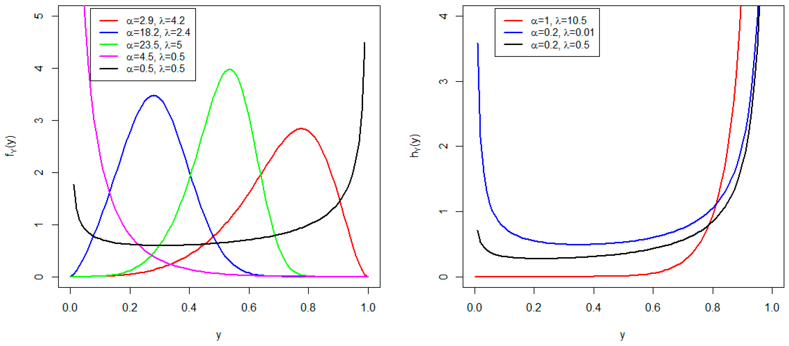
2. Bounded Truncated Cauchy Power Exponential Distribution
3. Some Important Properties
3.1. Distribution Inequalities
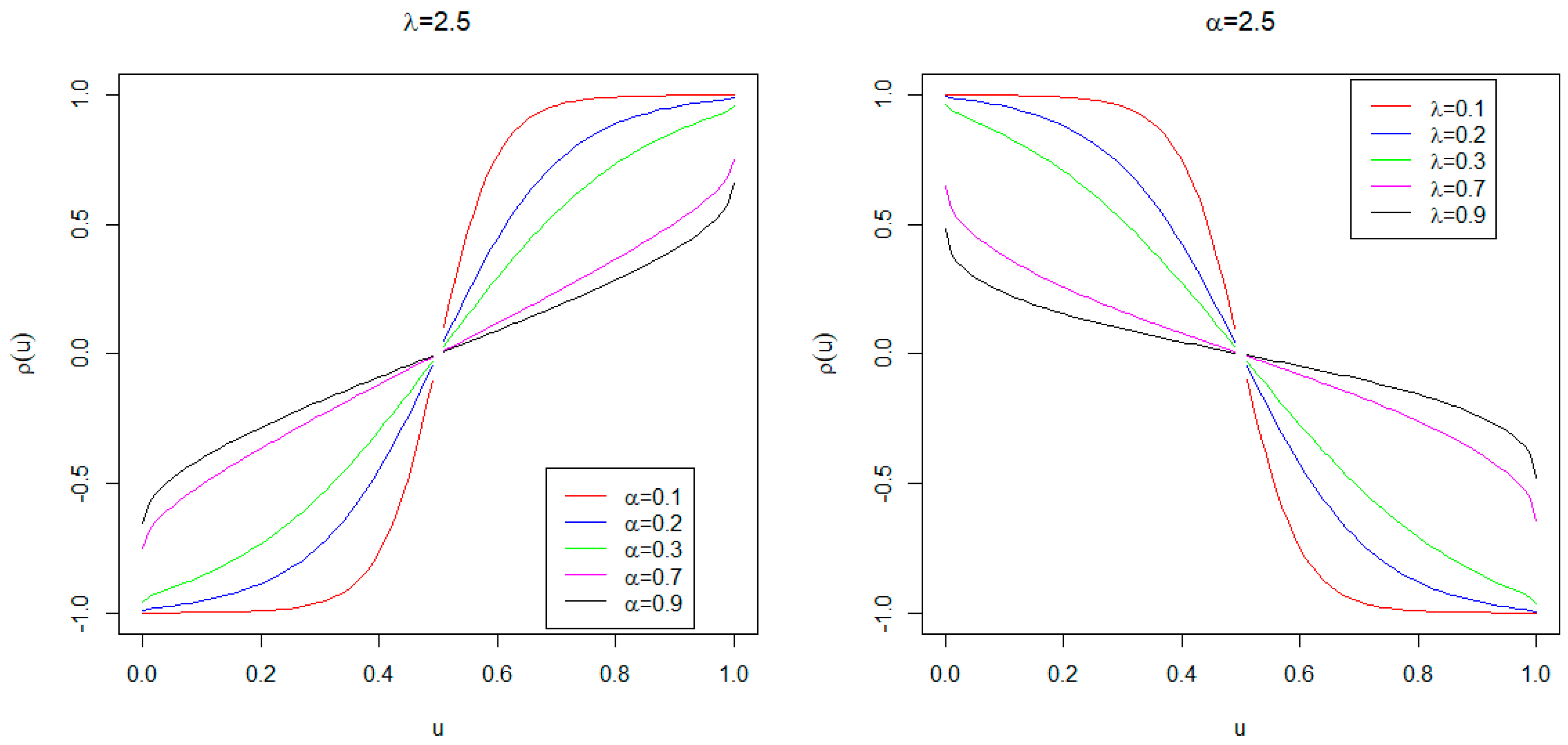
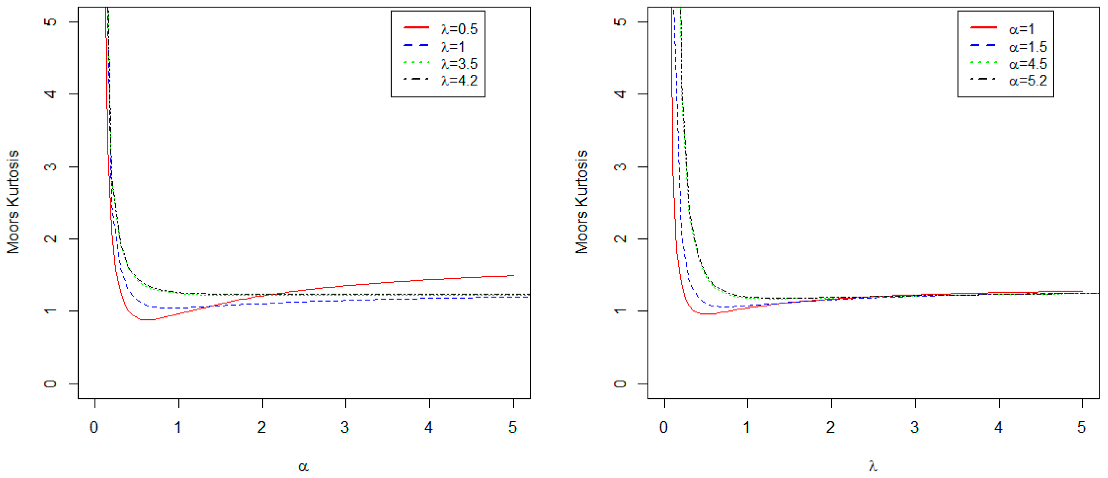
3.2. Quantile Function
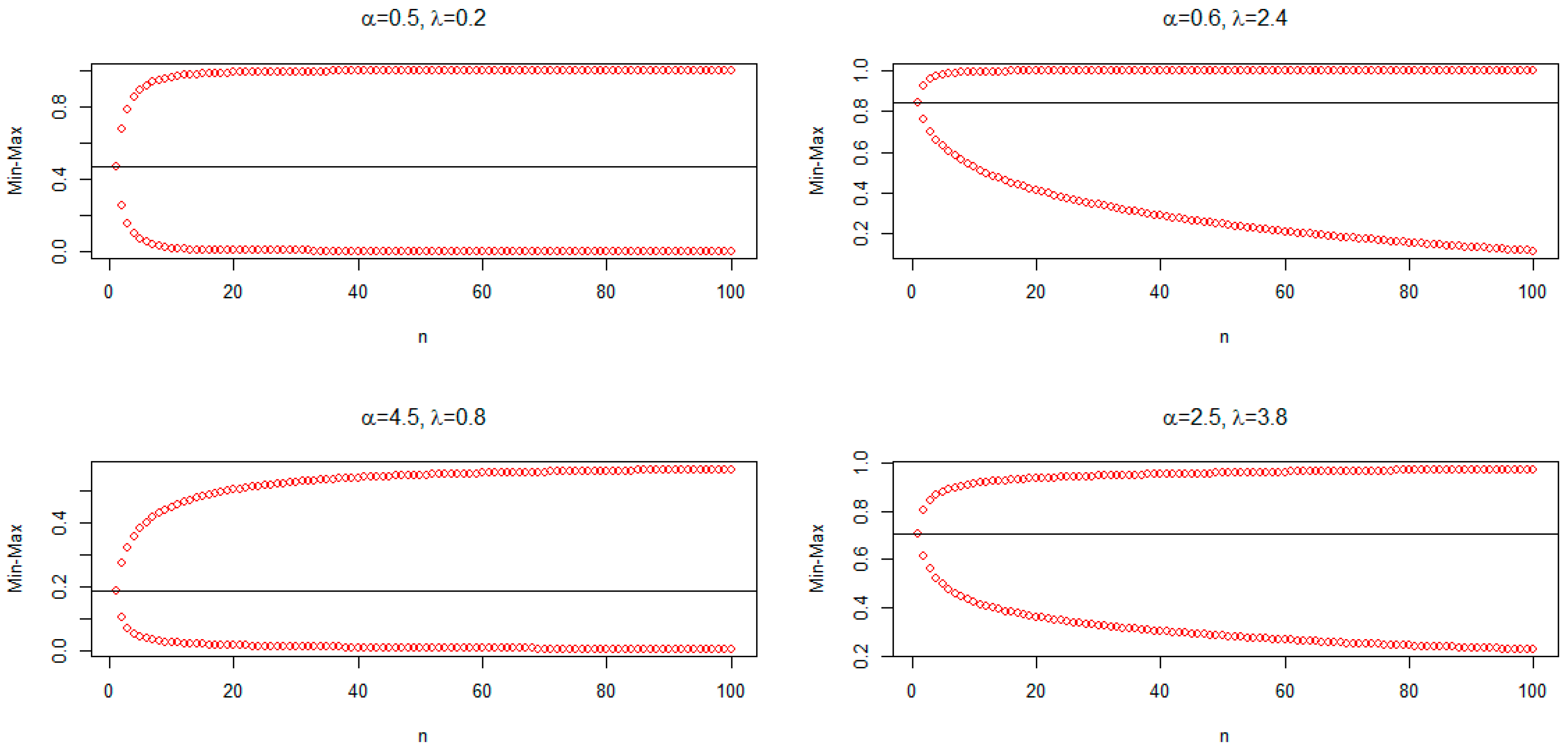
3.3. Moments and Moments Generating Function
3.4. Order Statistics
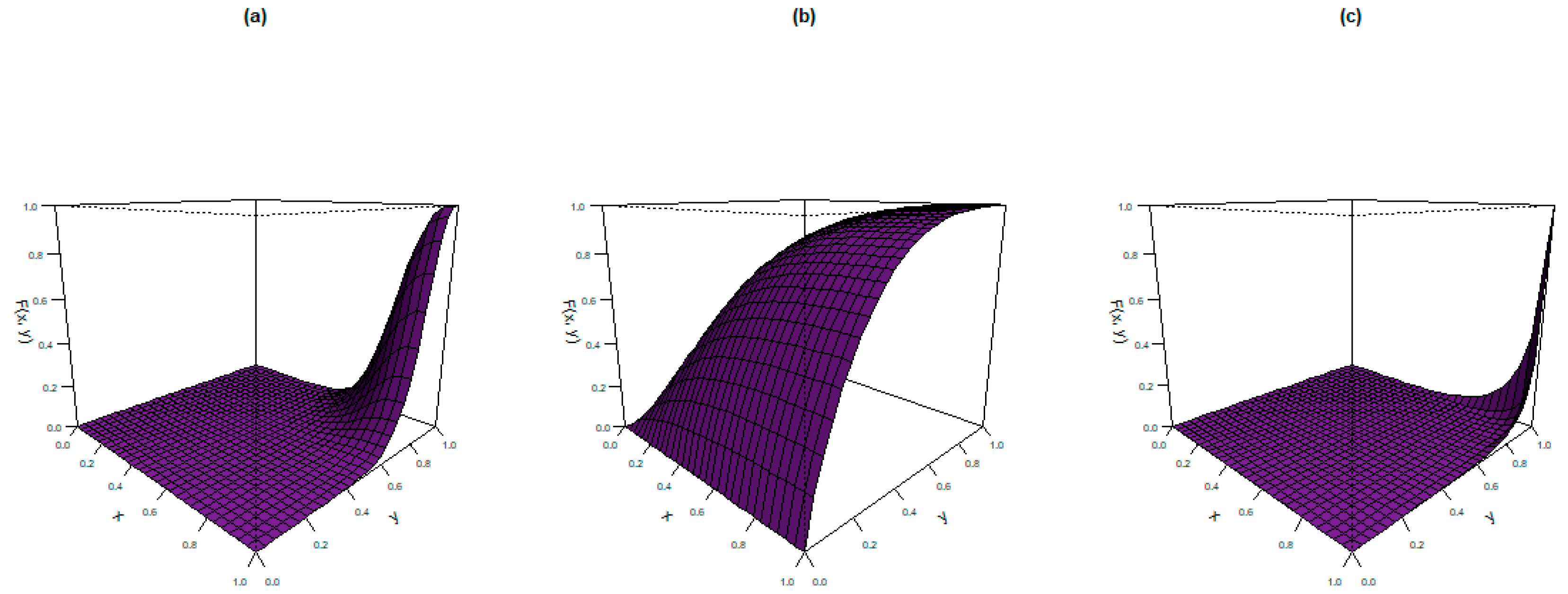
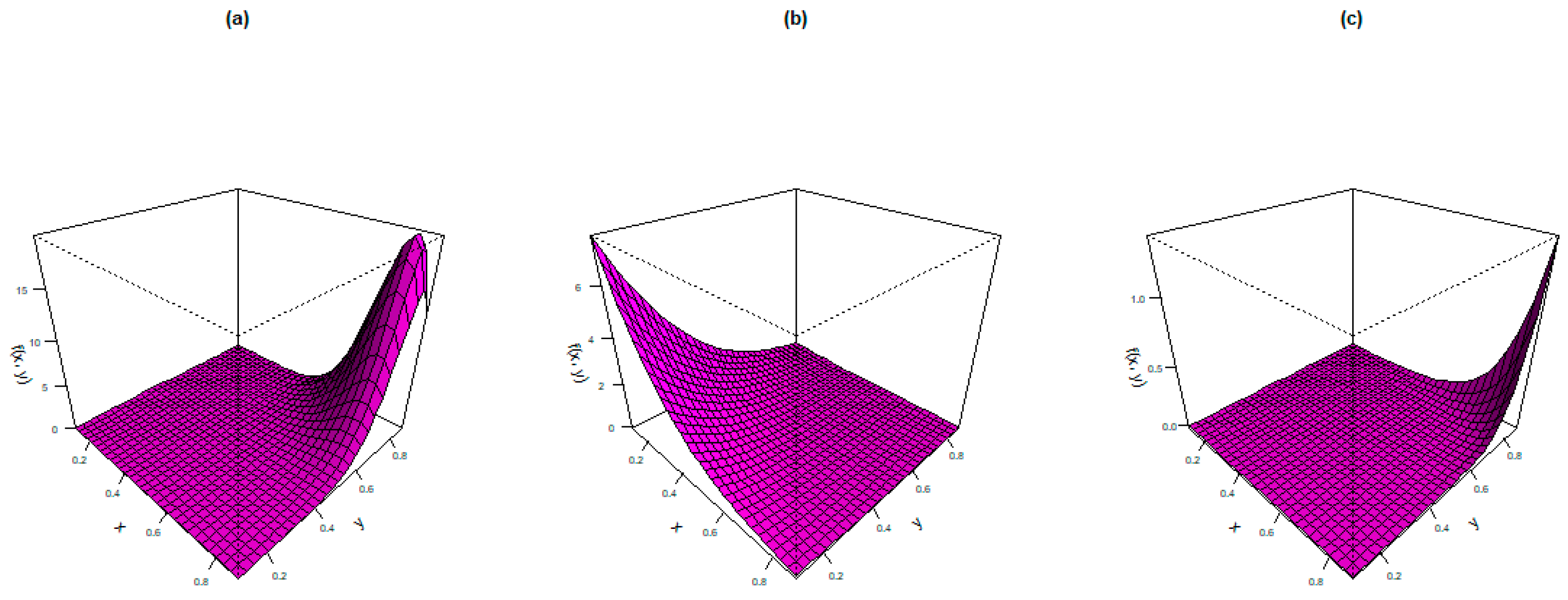
4. Bivariate Extension
- (a)
- ;
- (b)
- and
- (c)
- .
- (a)
- ;
- (b)
- and
- (c)
- .
5. Parameter Estimation Methods
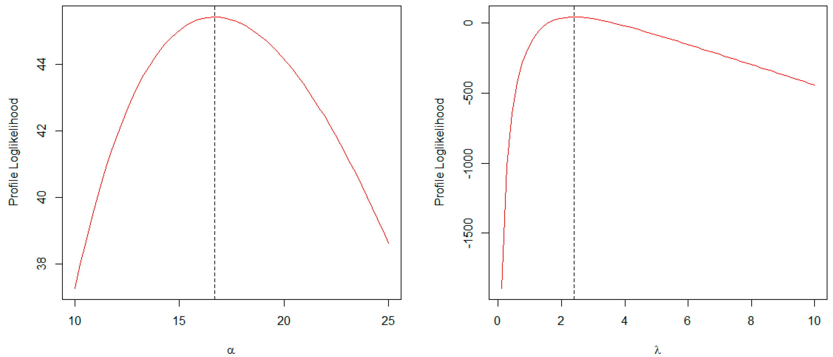
5.1. Maximum Likelihood Estimation
5.2. Ordinary and Weighted Least Squares Estimation
5.3. Cramér–Von Mises Estimation
5.4. Anderson–Darling Estimation
5.5. Percentile Estimation
5.6. Maximum and Minimum Product Spacing Estimation
6. Simulation
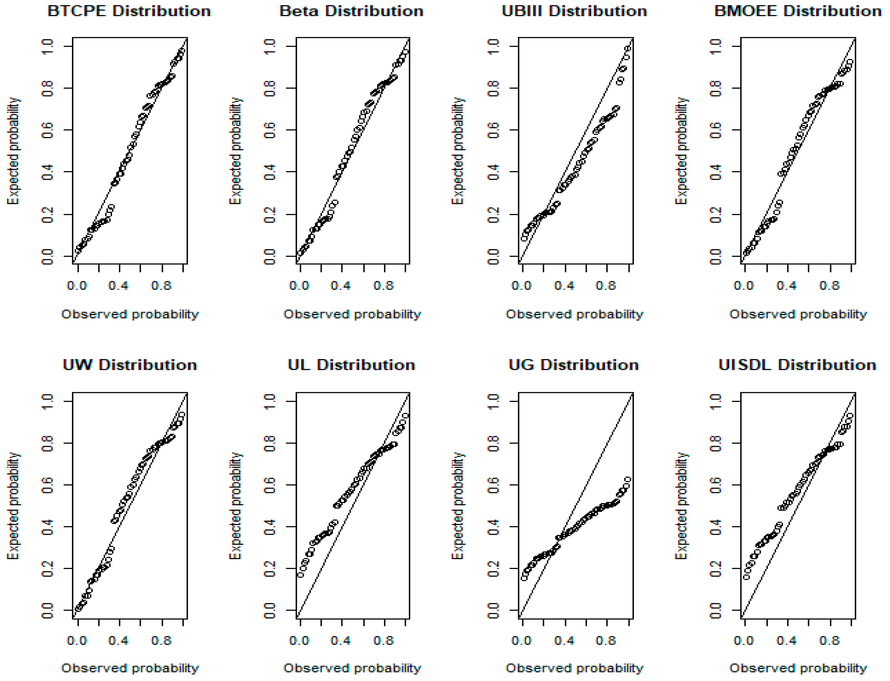
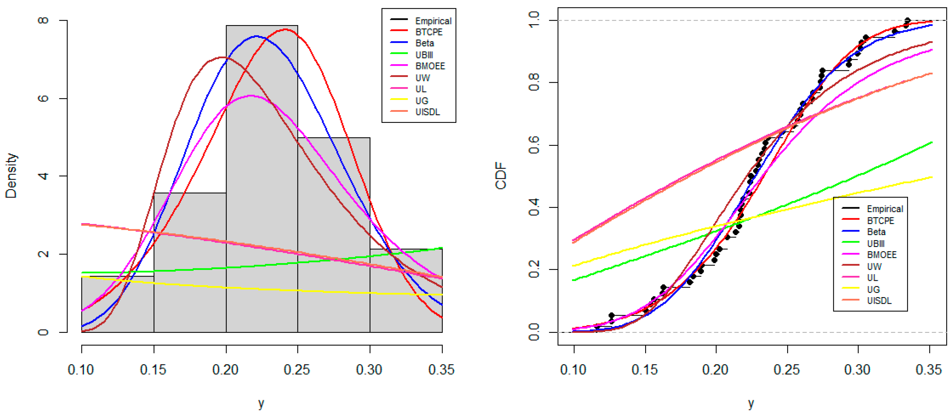
7. Applications
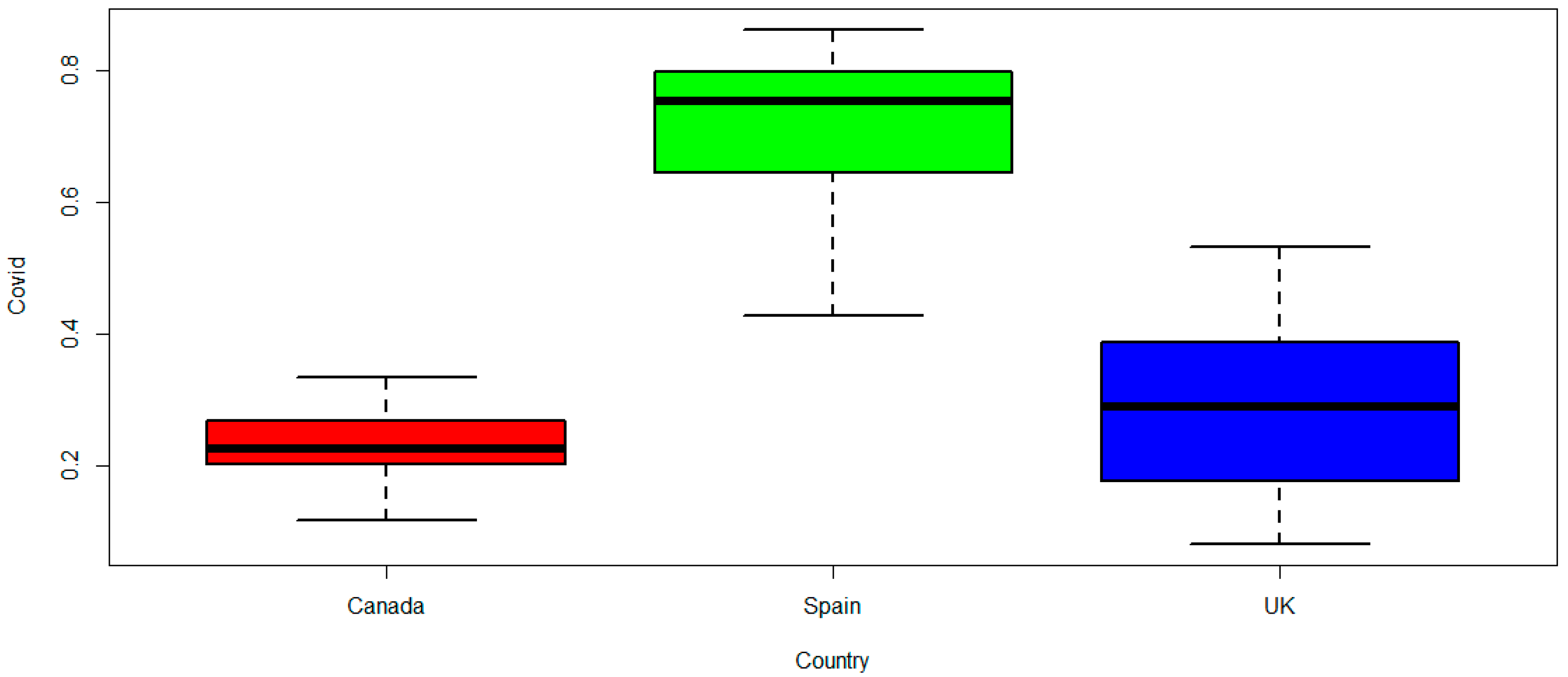
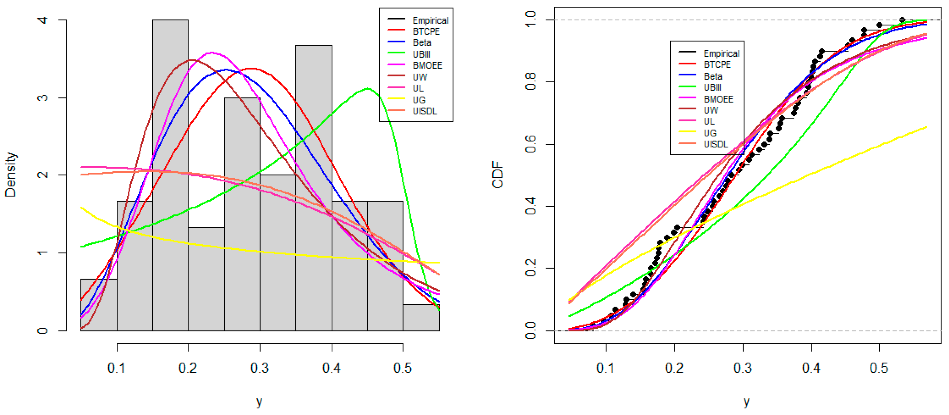
7.1. UK COVID-19 Mortality
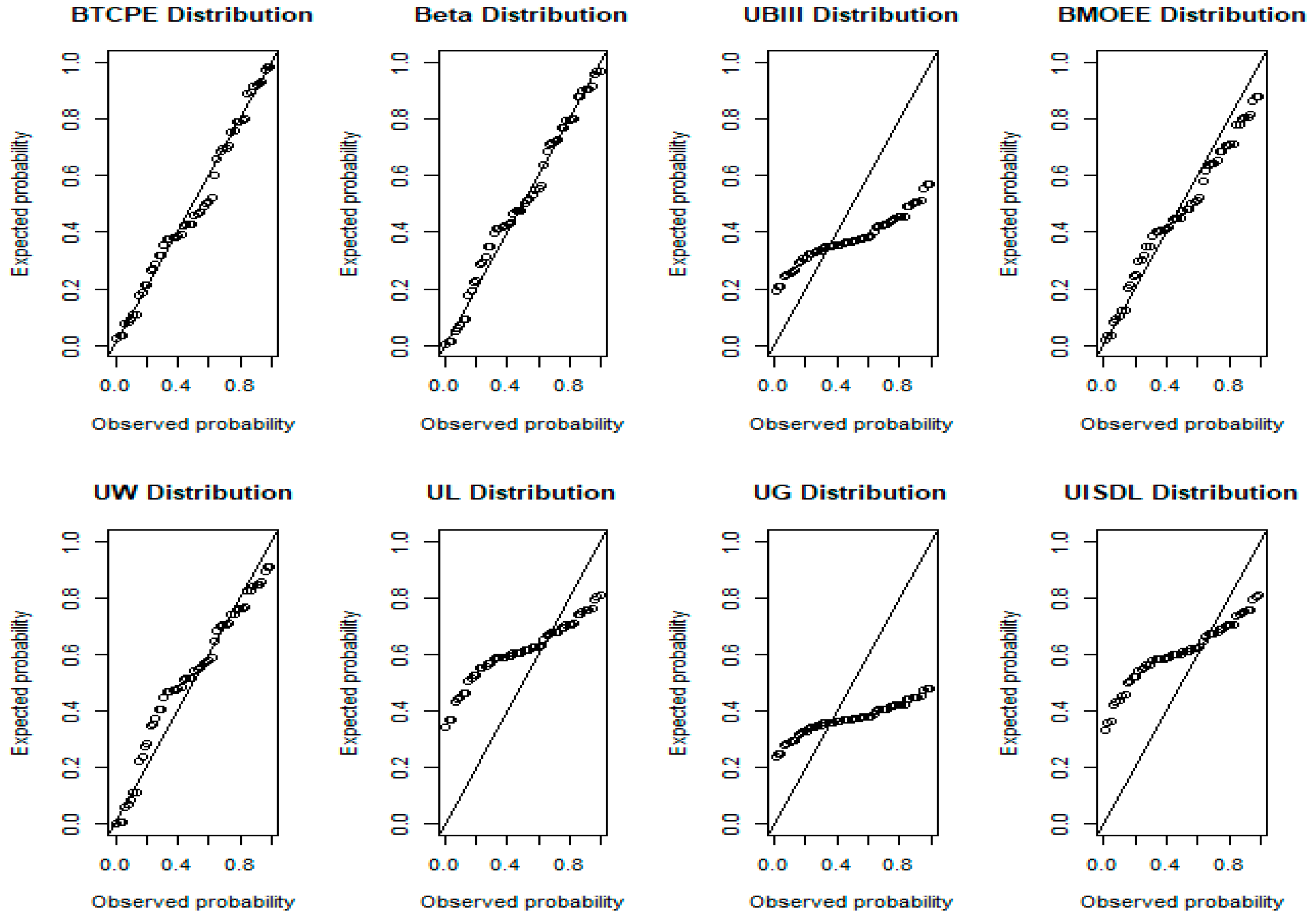
7.2. Canada COVID-19 Mortality
7.3. Spain COVID-19 Recovery Rate
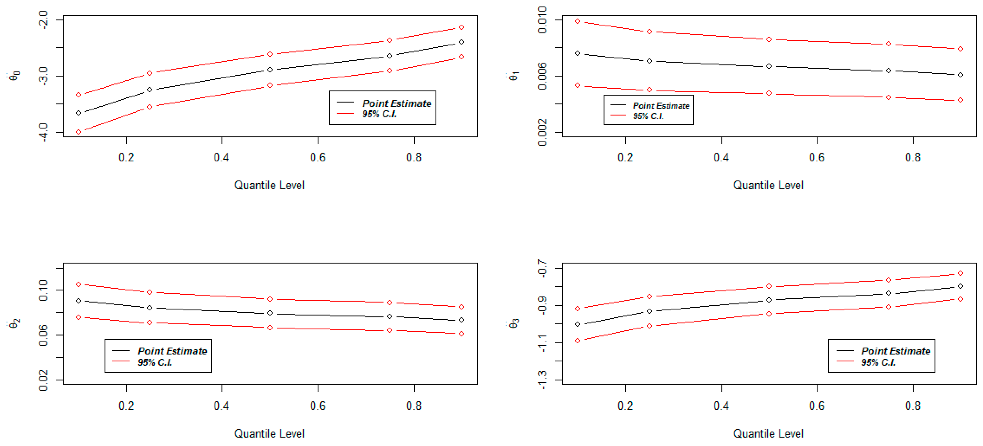
8. Quantile Regression
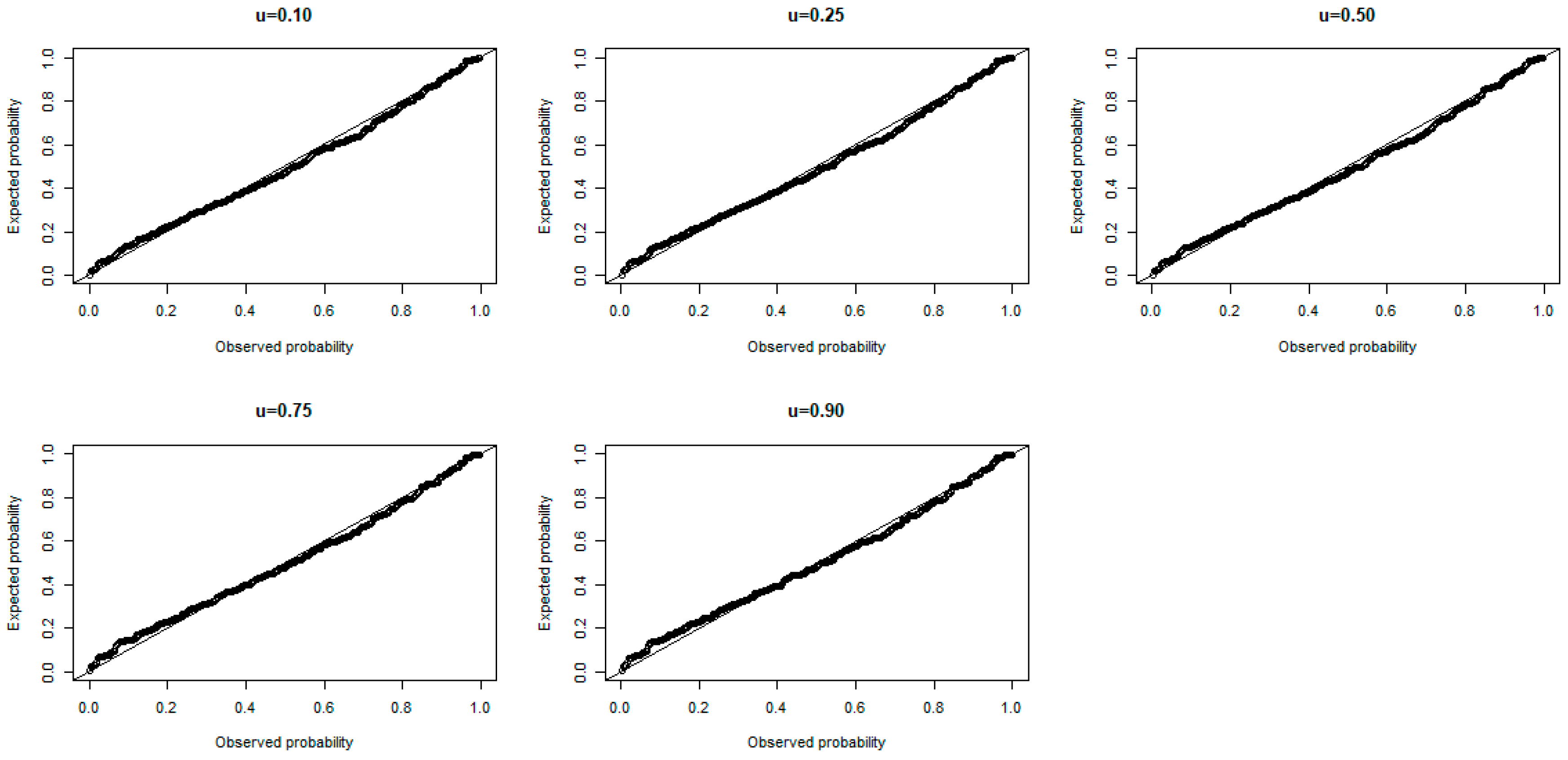
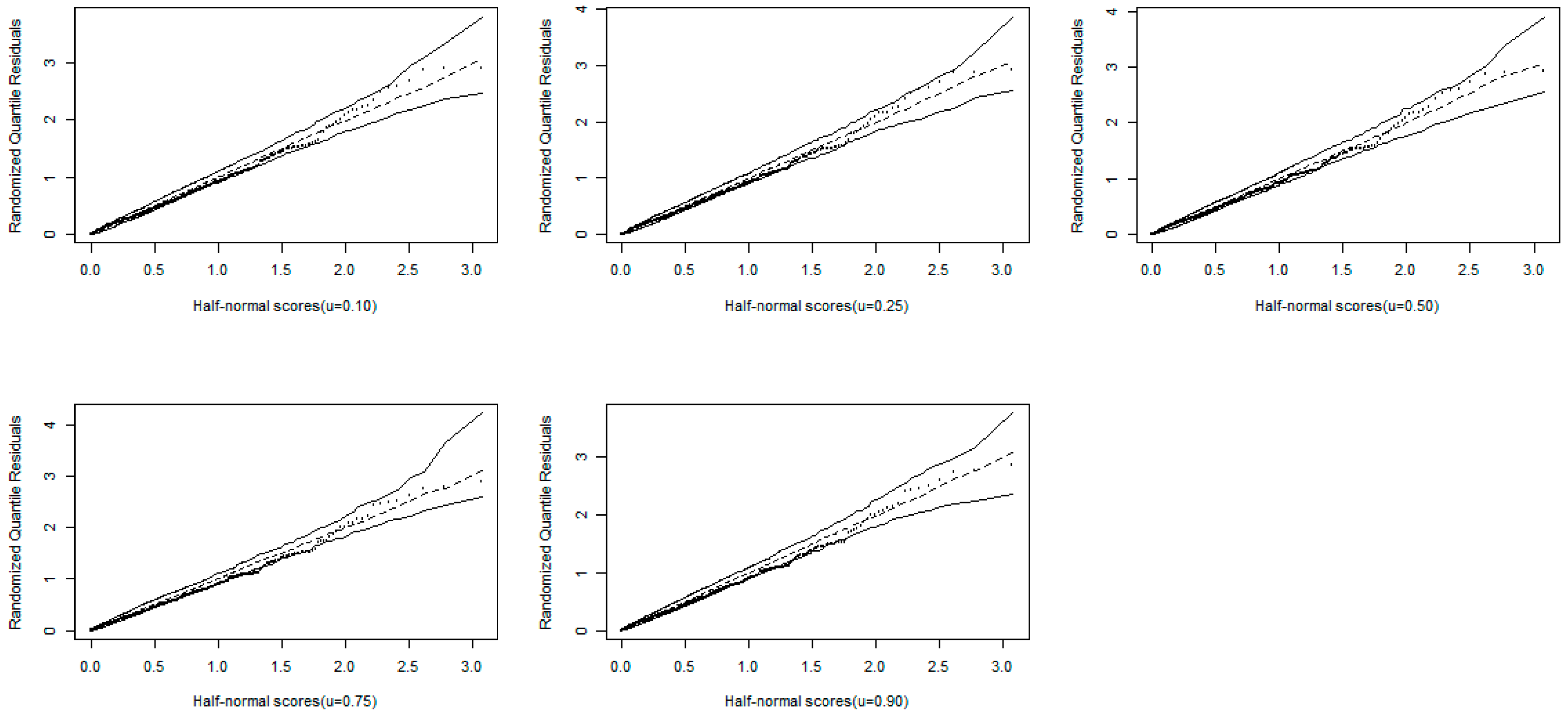
8.1. Residual Analysis
8.2. Monte Carlo Simulation for Quantile Regression
8.3. Application
9. Conclusions
Author Contributions
Funding
Conflicts of Interest
References
- Afify, A.Z.; Nassar, M.; Kumar, D.; Cordeiro, G.M. A new unit distribution: Properties and applications. Electron. J. Appl. Stat. Anal. 2022, 15, 460–484. [Google Scholar]
- Almazah, M.M.A.; Ullah, K.; Hussam, E.; Hossain, M.; Aldallal, R.; Riad, F.H. New Statistical Approaches for Modeling the COVID-19 Data Set: A Case Study in the Medical Sector. Complexity 2022, 2022, 1325825. [Google Scholar] [CrossRef]
- Alahmadi, A.A.; Alqawba, M.; Almutiry, W.; Shawki, A.W.; Alrajhi, S.; Al-Marzouki, S.; Elgarhy, M. A New Version of Weighted Weibull Distribution: Modelling to COVID-19 Data. Discret. Dyn. Nat. Soc. 2022, 2022, 3994361. [Google Scholar] [CrossRef]
- Algarni, A.; Almarashi, A.M.; Elbatal, I.; Hassan, A.S.; Almetwally, E.M.; Daghistani, A.M.; Elgarhy, M. Type I Half Logistic Burr X-G Family: Properties, Bayesian, and Non-Bayesian Estimation under Censored Samples and Applications to COVID-19 Data. Math. Probl. Eng. 2021, 2021, 5461130. [Google Scholar] [CrossRef]
- Bantan, R.A.R.; Shafiq, S.; Tahir, M.H.; Elhassanein, A.; Jamal, F.; Almutiry, W.; Elgarhy, M. Statistical Analysis of COVID-19 Data: Using a New Univariate and Bivariate Statistical Model. J. Funct. Spaces 2022, 2022, 2851352. [Google Scholar] [CrossRef]
- Arif, M.; Khan, D.M.; Aamir, M.; Khalil, U.; Bantan, R.A.R.; Elgarhy, M. Modeling COVID-19 Data with a Novel Extended Exponentiated Class of Distributions. J. Math. 2022, 2022, 1908161. [Google Scholar] [CrossRef]
- Nagy, M.; Almetwally, E.M.; Gemeay, A.M.; Mohammed, H.S.; Jawa, T.M.; Sayed-Ahmed, N.; Muse, A.H. The New Novel Discrete Distribution with Application on COVID-19 Mortality Numbers in Kingdom of Saudi Arabia and Latvia. Complexity 2021, 2021, 7192833. [Google Scholar] [CrossRef]
- Almetwally, E.M. The Odd Weibull Inverse Topp–Leone Distribution with Applications to COVID-19 Data. Ann. Data Sci. 2021, 9, 121–140. [Google Scholar] [CrossRef]
- Muse, A.H.; Tolba, A.H.; Fayad, E.; Abu Ali, O.A.; Nagy, M.; Yusuf, M. Modelling the COVID-19 Mortality Rate with a New Versatile Modification of the Log-Logistic Distribution. Comput. Intell. Neurosci. 2021, 2021, 8640794. [Google Scholar] [CrossRef]
- Haq, M.A.U.; Babar, A.; Hashmi, S.; Alghamdi, A.S.; Afify, A.Z. The Discrete Type-II Half-Logistic Exponential Distribution with Applications to COVID-19 Data. Pak. J. Stat. Oper. Res. 2021, 17, 921–932. [Google Scholar] [CrossRef]
- Gündüz, S.; Korkmaz, M. A New Unit Distribution Based on the Unbounded Johnson Distribution Rule: The Unit Johnson SU Distribution. Pak. J. Stat. Oper. Res. 2020, 16, 471–490. [Google Scholar] [CrossRef]
- Bantan, R.; Jamal, F.; Chesneau, C.; Elgarhy, M. Theory and Applications of the Unit Gamma/Gompertz Distribution. Mathematics 2021, 9, 1850. [Google Scholar] [CrossRef]
- Nasiru, S.; Abubakari, A.G.; Angbing, I.D. Bounded Odd Inverse Pareto Exponential Distribution: Properties, Estimation, and Regression. Int. J. Math. Math. Sci. 2021, 2021, 9955657. [Google Scholar] [CrossRef]
- Jodrá, P. A bounded distribution derived from the shifted Gompertz law. J. King Saud Univ.-Sci. 2020, 32, 523–536. [Google Scholar] [CrossRef]
- Haq, M.A.U.; Hashmi, S.; Aidi, K.; Ramos, P.L.; Louzada, F. Unit Modified Burr-III Distribution: Estimation, Characterizations and Validation Test. Ann. Data Sci. 2020, 99, 1–26. [Google Scholar] [CrossRef]
- Korkmaz, M.Ç. The unit generalized half normal distribution: A new bounded distribution with inference and application. U. P. B. Sci. Bull. Ser. A 2020, 82, 133–140. [Google Scholar]
- Mazucheli, J.; Menezes, A.F.B.; Chakraborty, S. On the one parameter unit-Lindley distribution and its associated regression model for proportion data. J. Appl. Stat. 2019, 46, 700–714. [Google Scholar] [CrossRef]
- Mazucheli, J.; Menezes, A.F.; Dey, S. Unit-Gompertz distribution with applications. Statistica 2019, 79, 25–43. [Google Scholar]
- Korkmaz, M. A new heavy-tailed distribution defined on the bounded interval. J. Appl. Stat. 2019, 47, 2097–2119. [Google Scholar] [CrossRef]
- Mazucheli, J.; Menezes, A.F.; Ghitany, M.E. The unit Weibull distribution and associated inference. J. Appl. Probab. Stat. 2018, 13, 1–22. [Google Scholar]
- Ghitany, M.E.; Mazucheli, J.; Menezes, A.F.B.; Alqallaf, F. The unit-inverse Gaussian distribution: A new alternative to two-parameter distributions on the unit interval. Commun. Stat.-Theory Methods 2018, 48, 3423–3438. [Google Scholar] [CrossRef]
- Aldahlan, M.A.; Jamal, F.; Chesneau, C.; Elgarhy, M.; Elbatal, I. The Truncated Cauchy Power Family of Distributions with Inference and Applications. Entropy 2020, 22, 346. [Google Scholar] [CrossRef] [PubMed]
- Shaked, M.; Shanthikumar, J.G. Stochastic Orders; Wiley: New York, NY, USA, 2007. [Google Scholar]
- MacGillivray, H.L. Skewness and Asymmetry: Measures and Orderings. Ann. Stat. 1986, 14, 994–1011. [Google Scholar] [CrossRef]
- Moors, J.J. A quantile alternative for kurtosis. J. R. Stat. Soc. Ser. D 1988, 37, 25–32. [Google Scholar] [CrossRef]
- Elhassanein, A. On Statistical Properties of a New Bivariate Modified Lindley Distribution with an Application to Financial Data. Complexity 2022, 2022, 2328831. [Google Scholar] [CrossRef]
- Ganji, M.; Bevrani, H.; Hami, N. A New Method For Generating Continuous Bivariate Families. J. Iran. Stat. Soc. 2018, 17, 109–129. [Google Scholar] [CrossRef]
- R Core Team. R: A Language and Environment for Statistical Computing; R Foundation for Statistical Computing: Vienna, Austria, 2019; Available online: https://www.R-project.org/ (accessed on 30 October 2022).
- Modi, K.; Gill, V. Unit Burr-III distribution with application. J. Stat. Manag. Syst. 2019, 23, 579–592. [Google Scholar] [CrossRef]
- Ghosh, I.; Dey, S.; Kumar, D. Bounded M-O Extended Exponential Distribution with Applications. Stoch. Qual. Control 2019, 34, 35–51. [Google Scholar] [CrossRef]
- Altun, E.; Cordeiro, G.M. The unit-improved second-degree Lindley distribution: Inference and regression modeling. Comput. Stat. 2019, 35, 259–279. [Google Scholar] [CrossRef]
- Bolker, B. Tools for General Maximum Likelihood Estimation; R Development Core Team: Vienna, Austria, 2014. Available online: https://github.com/bbolker/bbmle (accessed on 30 October 2022).
- Xiang, Y.; Gubian, S.; Suomela, B.; Hoeng, J. Generalized simulated annealing: GenSA package. R J. 2013, 5, 13–29. [Google Scholar] [CrossRef]
- Petterle, R.R.; Bonat, W.H.; Scarpin, C.T.; Jonasson, T.; Borba, V.Z.C. Multivariate quasi-beta regression models for continuous bounded data. Int. J. Biostat. 2020, 17, 39–53. [Google Scholar] [CrossRef] [PubMed]


| 0.8799 | 0.5602 | 0.1339 | |
| 0.8021 | 0.3401 | 0.0242 | |
| 0.7457 | 0.2185 | 0.0053 | |
| 0.7020 | 0.1465 | 0.0013 | |
| 0.6667 | 0.1017 | 0.0004 | |
| 0.6373 | 0.0726 | 0.0001 | |
| SD | 0.1668 | 0.1619 | 0.0794 |
| CV | 0.1896 | 0.2890 | 0.5931 |
| CS | −1.9527 | −0.3403 | 0.7713 |
| CK | 6.6850 | 2.7084 | 3.5390 |
| Parameter | AB | RMSE | |||||||||||||||||
|---|---|---|---|---|---|---|---|---|---|---|---|---|---|---|---|---|---|---|---|
| MLE | MPS | MADS | MALDS | OLS | WLS | CVM | AD | PC | MLE | MPS | MADS | MALDS | OLS | WLS | CVM | AD | PC | ||
| 25 | 0.7980 | 2.2327 | −2.3189 | 0.531 | 0.3530 | −2.6423 | 1.1477 | 0.4713 | −0.3155 | 2.2233 | 3.5728 | 2.9322 | 3.3391 | 2.4457 | 2.6729 | 3.5377 | 1.9964 | 1.4972 | |
| 75 | 0.2140 | 0.7443 | −1.8442 | 0.0634 | 0.1365 | −3.1632 | 0.3415 | 0.1180 | −0.1694 | 0.9157 | 1.3139 | 2.4241 | 1.1330 | 1.1489 | 3.1657 | 1.2820 | 0.9535 | 0.8506 | |
| 125 | 0.1342 | 0.4372 | −1.3088 | −0.0031 | 0.0472 | −3.3268 | 0.1337 | 0.0713 | −0.0783 | 0.6843 | 0.8313 | 1.9860 | 0.7795 | 0.8149 | 3.3279 | 0.8159 | 0.7025 | 0.6641 | |
| 175 | 0.0914 | 0.2987 | −0.8738 | −0.0272 | 0.0460 | −2.1721 | 0.1164 | 0.0657 | −0.0484 | 0.5365 | 0.6791 | 1.5544 | 0.6323 | 0.6845 | 2.1990 | 0.6955 | 0.5941 | 0.5393 | |
| 225 | 0.0677 | 0.2509 | −0.6976 | 0.0062 | 0.0301 | 3.0791 | 0.1096 | 0.0365 | −0.0623 | 0.4841 | 0.5505 | 1.3266 | 0.5926 | 0.5906 | 3.3377 | 0.6147 | 0.5240 | 0.4860 | |
| 25 | 0.1871 | 0.5436 | −1.1017 | 0.0300 | −0.0075 | −1.3344 | 0.2060 | 0.0670 | −0.1737 | 0.6038 | 0.8201 | 1.3862 | 0.7382 | 0.6538 | 1.3687 | 0.7340 | 0.5749 | 0.5401 | |
| 75 | 0.0478 | 0.2197 | −0.8939 | −0.0079 | 0.0078 | −2.0003 | 0.0802 | 0.1185 | −0.0672 | 0.3089 | 0.4026 | 1.2090 | 0.3996 | 0.3692 | 2.0029 | 0.3886 | 0.3379 | 0.3175 | |
| 125 | 0.0378 | 0.1293 | −0.6271 | −0.0160 | −0.0055 | −2.1461 | 0.0305 | 0.0146 | −0.0448 | 0.2407 | 0.2740 | 0.9681 | 0.2987 | 0.2752 | 2.1472 | 0.2798 | 0.2560 | 0.2466 | |
| 175 | 0.0233 | 0.0866 | −0.3986 | −0.0139 | 0.0034 | −1.6394 | 0.0280 | 0.0114 | −0.0267 | 0.1959 | 0.2314 | 0.7264 | 0.2315 | 0.2372 | 1.6455 | 0.2383 | 0.2134 | 0.2008 | |
| 225 | 0.0208 | 0.0820 | −0.3101 | 0.0021 | 0.0003 | 0.1937 | 0.0230 | 0.0007 | −0.0225 | 0.1810 | 0.1939 | 0.6057 | 0.2196 | 0.2079 | 0.3066 | 0.2124 | 0.1874 | 0.1835 | |
| Parameter | AB | RMSE | |||||||||||||||||
|---|---|---|---|---|---|---|---|---|---|---|---|---|---|---|---|---|---|---|---|
| MLE | MPS | MADS | MALDS | OLS | WLS | CVM | AD | PC | MLE | MPS | MADS | MALDS | OLS | WLS | CVM | AD | PC | ||
| 25 | 0.5120 | 1.5281 | −1.3158 | 0.3712 | 0.2359 | −1.9121 | 0.7701 | 0.2725 | −0.6748 | 1.4793 | 2.5597 | 2.0817 | 1.9689 | 1.6086 | 1.9366 | 2.4325 | 1.3231 | 1.4204 | |
| 75 | 0.2081 | 0.5190 | −0.9456 | 0.0477 | 0.0264 | −2.2924 | 0.1973 | 0.0989 | −0.3302 | 0.6848 | 0.8671 | 1.5913 | 0.7865 | 0.7088 | 2.2949 | 0.8122 | 0.6294 | 0.8145 | |
| 125 | 0.0994 | 0.3218 | −0.6895 | 0.0570 | 0.0153 | −2.4255 | 0.1020 | 0.0757 | −0.2704 | 0.4778 | 0.6228 | 1.2854 | 0.5657 | 0.5532 | 2.4266 | 0.5644 | 0.5109 | 0.6262 | |
| 175 | 0.0867 | 0.2259 | −0.5478 | 0.0107 | 0.0240 | −1.3857 | 0.0882 | 0.0554 | −0.2187 | 0.4077 | 0.4554 | 1.0538 | 0.4821 | 0.4813 | 1.4810 | 0.4940 | 0.4163 | 0.5242 | |
| 225 | 0.0461 | 0.1719 | −0.4192 | 0.0007 | 0.0195 | 2.2166 | 0.0555 | 0.0200 | −0.1735 | 0.3331 | 0.3880 | 0.8460 | 0.4021 | 0.4133 | 2.3785 | 0.4184 | 0.3477 | 0.4768 | |
| 25 | 0.5725 | 1.9602 | −3.5282 | 0.1675 | 0.1107 | −4.6443 | 0.7293 | 0.2368 | −1.6432 | 2.0951 | 3.1555 | 4.8358 | 2.6753 | 2.3883 | 4.7703 | 2.6517 | 2.1203 | 2.6346 | |
| 75 | 0.2957 | 0.8211 | −2.4563 | −0.0292 | −0.0416 | −6.9243 | 0.2449 | 0.0825 | −0.7220 | 1.1627 | 1.4130 | 3.9050 | 1.3676 | 1.2655 | 6.9330 | 1.3246 | 1.1047 | 1.4877 | |
| 125 | 0.1098 | 0.4964 | −1.6975 | 0.0128 | −0.0435 | −7.3960 | 0.1015 | 0.0784 | −0.5259 | 0.8837 | 1.0321 | 3.0631 | 1.0694 | 0.9899 | 7.3994 | 0.9670 | 0.9327 | 1.1482 | |
| 175 | 0.1182 | 0.3504 | −1.2348 | −0.0232 | 0.0022 | −5.5678 | 0.1061 | 0.0622 | −0.4011 | 0.7361 | 0.7786 | 2.4368 | 0.8864 | 0.8608 | 5.5937 | 0.8687 | 0.7734 | 0.9365 | |
| 225 | 0.0631 | 0.2843 | −0.9196 | −0.0034 | 0.0015 | 0.6715 | 0.043 | 0.0249 | −0.3171 | 0.6223 | 0.7091 | 1.9241 | 0.7604 | 0.7452 | 1.0898 | 0.7515 | 0.6590 | 0.8305 | |
| Country | Minimum | Maximum | Mean | Skewness | Kurtosis |
|---|---|---|---|---|---|
| UK | 0.0807 | 0.5331 | 0.2888 | 0.0476 | −1.1034 |
| Canada | 0.1159 | 0.3347 | 0.2305 | −0.0850 | −0.4402 |
| Spain | 0.4286 | 0.8628 | 0.7240 | −0.6890 | −0.4761 |
| Model | Parameter | AIC | BIC | AD | CVM | |
|---|---|---|---|---|---|---|
| BTCPE | 45.4400 | −86.8726 | −82.6840 | 0.6494 | 0.1049 | |
| Beta | 45.4000 | −86.7958 | −82.6071 | 0.7356 | 0.1280 | |
| UBIII | 38.9000 | −73.8075 | −69.6188 | 2.8948 | 0.5248 | |
| BMOEE | 40.7200 | −77.4396 | −73.2509 | 1.1465 | 0.1698 | |
| UW | 42.5600 | −81.1208 | −76.9322 | 1.0656 | 0.1820 | |
| UG | 2.8400 | −1.6760 | 2.5127 | 12.2290 | 2.4707 | |
| UL | 32.3800 | −62.7533 | −60.6590 | 4.4878 | 0.7574 | |
| UISDL | 33.6100 | −65.2142 | −63.1198 | 3.9972 | 0.6545 |
| Model | Parameter | AIC | BIC | AD | CVM | |
|---|---|---|---|---|---|---|
| BTCPE | 86.4400 | −168.8806 | −164.8299 | 0.3767 | 0.0689 | |
| Beta | 85.9400 | −167.8800 | −163.8293 | 0.4398 | 0.0692 | |
| UBIII | 30.8900 | −57.7749 | −53.7242 | 14.8770 | 3.1113 | |
| BMOEE | 80.6700 | −157.3394 | −153.2887 | 1.5514 | 0.2327 | |
| UW | 79.9500 | −155.9080 | −151.8573 | 1.4890 | 0.2389 | |
| UG | 5.2500 | −6.4901 | −2.4393 | 18.5180 | 3.9712 | |
| UL | 41.1400 | −80.2707 | −78.2453 | 12.7090 | 2.5936 | |
| UISDL | 42.2000 | −82.3913 | −80.3660 | 12.3010 | 2.4925 |
| Model | Parameter | AIC | BIC | AD | CVM | |
|---|---|---|---|---|---|---|
| BTCPE | 58.7500 | −113.4953 | −109.1160 | 0.8770 | 0.1363 | |
| Beta | 57.5700 | −111.1489 | −106.7692 | 1.0520 | 0.1783 | |
| UBIII | 53.8000 | −103.5927 | −99.2134 | 1.3725 | 0.2209 | |
| BMOEE | 51.4600 | −98.9276 | −94.5483 | 1.4958 | 0.2100 | |
| UW | 53.9700 | −103.9316 | −99.5523 | 1.3830 | 0.2238 | |
| UG | 46.0300 | −88.0569 | −83.6776 | 2.4709 | 0.3691 | |
| UL | 46.1100 | −90.2298 | −88.0402 | 4.2480 | 0.6736 | |
| UISDL | 52.0400 | −102.0717 | −99.8820 | 2.3450 | 0.3194 |
| I | II | III | |||||
|---|---|---|---|---|---|---|---|
| Parameter | n | AB | RMSE | AB | RMSE | AB | RMSE |
| 50 | 0.1949 | 0.2235 | 0.3599 | 0.3753 | 0.2609 | 0.2969 | |
| 100 | 0.1946 | 0.1961 | 0.3551 | 0.3726 | 0.2178 | 0.2579 | |
| 250 | 0.1919 | 0.1941 | 0.3465 | 0.3673 | 0.1525 | 0.1926 | |
| 350 | 0.1898 | 0.1928 | 0.3271 | 0.3544 | 0.1320 | 0.1700 | |
| 500 | 0.1838 | 0.1927 | 0.3109 | 0.3482 | 0.1101 | 0.1431 | |
| 600 | 0.1779 | 0.1886 | 0.3051 | 0.3434 | 0.0998 | 0.1318 | |
| 700 | 0.1761 | 0.1850 | 0.2908 | 0.3333 | 0.0908 | 0.1196 | |
| 50 | 0.2826 | 0.3067 | 0.3485 | 0.3807 | 0.8194 | 0.8276 | |
| 100 | 0.2605 | 0.2904 | 0.3181 | 0.3486 | 0.8142 | 0.8238 | |
| 250 | 0.2290 | 0.2651 | 0.3171 | 0.3363 | 0.8013 | 0.8134 | |
| 350 | 0.2176 | 0.2539 | 0.3138 | 0.3342 | 0.7872 | 0.8041 | |
| 500 | 0.2097 | 0.2454 | 0.3083 | 0.3305 | 0.7727 | 0.7945 | |
| 600 | 0.2079 | 0.2433 | 0.3020 | 0.3272 | 0.7188 | 0.7610 | |
| 700 | 0.2053 | 0.2389 | 0.2978 | 0.3253 | 0.6862 | 0.7447 | |
| 50 | 1.5889 | 1.5959 | 1.7104 | 1.7153 | 0.5212 | 0.5338 | |
| 100 | 1.5835 | 1.5913 | 1.7046 | 1.7102 | 0.5140 | 0.5291 | |
| 250 | 1.5818 | 1.5910 | 1.6938 | 1.7006 | 0.5073 | 0.5250 | |
| 350 | 1.5698 | 1.5815 | 1.6751 | 1.6845 | 0.4893 | 0.5130 | |
| 500 | 1.5566 | 1.5723 | 1.6432 | 1.6578 | 0.4753 | 0.5046 | |
| 600 | 1.4749 | 1.5132 | 1.5559 | 1.5917 | 0.4601 | 0.4999 | |
| 700 | 1.3803 | 1.4520 | 1.4593 | 1.5264 | 0.4535 | 0.4921 | |
| 50 | 0.0792 | 0.0998 | 0.0842 | 0.1110 | 0.1091 | 0.1520 | |
| 100 | 0.0577 | 0.0745 | 0.0570 | 0.0747 | 0.0872 | 0.1382 | |
| 250 | 0.0352 | 0.0463 | 0.0339 | 0.0437 | 0.0523 | 0.0859 | |
| 350 | 0.0295 | 0.0378 | 0.0287 | 0.0366 | 0.0427 | 0.0650 | |
| 500 | 0.0246 | 0.0316 | 0.0239 | 0.0317 | 0.0340 | 0.0467 | |
| 600 | 0.0227 | 0.0287 | 0.0217 | 0.0290 | 0.0317 | 0.0449 | |
| 700 | 0.0210 | 0.0267 | 0.0201 | 0.0259 | 0.0287 | 0.0375 | |
| 0.10 | Estimates | −3.6699 | 0.0076 | 0.0905 | −1.004 | 308.7724 |
| Standard error | 0.1681 | |||||
| p-value | ||||||
| 0.25 | Estimates | −3.2544 | 0.0071 | 0.0845 | −0.9326 | 325.4705 |
| Standard error | 0.1545 | |||||
| p-value | ||||||
| 0.50 | Estimates | −2.8977 | 0.0067 | 0.0792 | −0.8732 | 340.4285 |
| Standard error | 0.1436 | |||||
| p-value | ||||||
| 0.75 | Estimates | −2.6424 | 0.0064 | 0.0766 | −0.8384 | 281.1611 |
| Standard error | 0.1405 | |||||
| p-value | ||||||
| 0.90 | Estimates | −2.4030 | 0.0061 | 0.0731 | −0.7987 | 273.9968 |
| Standard error | 0.1353 | |||||
| p-value |
| AIC | BIC | ||
|---|---|---|---|
| 0.10 | −885.3517 | −875.3517 | −856.8663 |
| 0.25 | −887.4067 | −877.4067 | −858.9212 |
| 0.50 | −889.1990 | −879.1990 | −860.7136 |
| 0.75 | −889.8634 | −879.8634 | −861.3779 |
| 0.90 | −890.8307 | −880.8307 | −862.3453 |
Publisher’s Note: MDPI stays neutral with regard to jurisdictional claims in published maps and institutional affiliations. |
© 2022 by the authors. Licensee MDPI, Basel, Switzerland. This article is an open access article distributed under the terms and conditions of the Creative Commons Attribution (CC BY) license (https://creativecommons.org/licenses/by/4.0/).
Share and Cite
Nasiru, S.; Abubakari, A.G.; Chesneau, C. New Lifetime Distribution for Modeling Data on the Unit Interval: Properties, Applications and Quantile Regression. Math. Comput. Appl. 2022, 27, 105. https://doi.org/10.3390/mca27060105
Nasiru S, Abubakari AG, Chesneau C. New Lifetime Distribution for Modeling Data on the Unit Interval: Properties, Applications and Quantile Regression. Mathematical and Computational Applications. 2022; 27(6):105. https://doi.org/10.3390/mca27060105
Chicago/Turabian StyleNasiru, Suleman, Abdul Ghaniyyu Abubakari, and Christophe Chesneau. 2022. "New Lifetime Distribution for Modeling Data on the Unit Interval: Properties, Applications and Quantile Regression" Mathematical and Computational Applications 27, no. 6: 105. https://doi.org/10.3390/mca27060105
APA StyleNasiru, S., Abubakari, A. G., & Chesneau, C. (2022). New Lifetime Distribution for Modeling Data on the Unit Interval: Properties, Applications and Quantile Regression. Mathematical and Computational Applications, 27(6), 105. https://doi.org/10.3390/mca27060105