A Front-Fixing Implicit Finite Difference Method for the American Put Options Model

Abstract

In this paper, we present an implicit finite difference method for the numerical solution of the Black–Scholes model of American put options without dividend payments. We combine the proposed numerical method by using a front-fixing approach where the option price and the early exercise boundary are computed simultaneously. We study the consistency and prove the stability of the implicit method by fixing the values of the free boundary and of its first derivative. We improve the accuracy of the computed solution via a mesh refinement based on Richardson’s extrapolation. Comparisons with some proposed methods for the American options problem are carried out to validate the obtained numerical results and to show the efficiency of the proposed numerical method. Finally, by using an a posteriori error estimator, we find a suitable computational grid requiring that the computed solution verifies a prefixed error tolerance.

1. Introduction

American options are contracts allowing the holder to exercise the option to sell or to buy an asset at a certain price at any time prior to and including its maturity date. The pricing of American options plays an important role both in theory and in real derivative markets. The option pricing model developed by Black and Scholes [1] and extended by Merton [2] has given rise to a partial differential equation governing the value of an option. Schwartz [3] and Brennan and Schwartz [4,5] were the first to apply a finite difference method to price American options. The accuracy of their finite difference method was proved by Jaillet et al. [6]. Other papers present finite difference methods (see, for example, Hull and White [7], Duffy [8], Wilmott et al. [9]). An alternative approach is based on front-tracking methods that keep track of the boundary and discretize the problem in changing domain; they have been considered in [10,11,12].

When we price an American option, we also need to determine the optimal exercise moment as a function of the value of the underlying asset. This leads to the formulation of a free boundary of the non-linear problem for the price of the American option when looking for a boundary that changes over time to maturity, known as the optimal exercise boundary. In particular, the American call option problem is a free boundary problem defined on a finite domain. On the other hand, the American put option problem is a free boundary problem that is defined on a semi-infinite domain, meaning that it is a non-linear model complicated by a boundary condition at infinity. The difficulty associated with a free boundary problem can be solved by using a front-fixing method—an approach relying on a change of variable to map the changing domain into a fixed domain.

The front-fixing approach has been considered in several papers. Holmes and Yang [13], used a front-fixing finite element method. Tangman et al. [12] introduced a fourth-order accurate finite difference scheme. In [14], the original problem was transformed into a more manageable equation with coefficients that are not dependent on the spatial variable, and an explicit update for the location of the free boundary at each time step was used; furthermore, in Zhu et al. [15], the secant method was employed to solve the non-linear problem. Moreover, in Tangman et al. [12,15], the difference between the prices of American options and European options was computed. Sevčovič [16] studied and approximated the early exercise boundary for a class of nonlinear Black–Scholes equations, applying a fixed-domain transformation and using an operator splitting iterative numerical technique. Lauko and Ševčovič [17] introduced a local iterative numerical scheme and compared analytical and numerical solutions for the early exercise boundary position computation of the American put option. In [18], Zhang and Zhu presented a predictor corrector method after the fixed-domain transformation. Nielsen et al. [19] used both explicit and implicit schemes to solve the Black–Scholes model of American options, while Company et al. [20] presented an explicit finite difference method for the free boundary value problem under logarithmic front-fixing transformation. In [21,22], Fazio proposed an a posteriori error estimator for the numerical solution to the American put option obtained by an explicit finite difference scheme.

In this paper, we present an implicit finite difference scheme combined with the use of the front-fixing method in order to solve the American put option problem without dividend payments. Preliminary results have been presented to the International Conference ICNAAM2015 [23]. We use a front-fixing variable transformation to reformulate the variable domain problem into a non-linear problem on a fixed rectangular domain. For the non-linear problem, we introduce a suitable choice of a truncated boundary that allows us to impose the asymptotic boundary condition. Then, the original problem is transformed into a new non-linear partial differential equation where the free boundary appears as a new variable and is computed as part of the solution. We develop an implicit finite difference method and we investigate the consistency and the stability property by fixing the values of the free boundary and of its first derivative.

Finally, we choose to validate the obtained numerical results via a mesh refinement and a Richardson’s extrapolation technique, and we present a comparison with numerical results available in the literature.

2. The American Put Options Model

Let us suppose that at time t the price of a given underlying asset is S. We consider here the following mathematical model for the value $P=P(S,\tau )$ of an American put option to sell the asset

$$\begin{array}{cc}\hfill & \frac{\partial P}{\partial \tau }=\frac{1}{2}{\sigma }^2{S}^2\frac{{\partial }^{2}P}{\partial S^2}+rS\frac{\partial P}{\partial S}-rP\mathrm{on}0<\tau \le T,S^{*}\left(\tau \right)<S<\infty ,\hfill \\ \hfill & P(S,0)=max(E-S,0),S^{*}\left(0\right)=E,\hfill \\ \hfill & \underset{S\to \infty }{lim}P(S,\tau )=0,\hfill \\ \hfill & P(S^{*}\left(\tau \right),\tau )=E-S^{*}\left(\tau \right),\frac{\partial P}{\partial S}(S^{*}\left(\tau \right),\tau )=-1,\hfill \\ \hfill & P(S,\tau )=E-S,0\le S<S^{*}\left(\tau \right),\hfill \end{array}$$

(1)

where $\tau =T-t$ denotes the time to maturity T, $S^{*}\left(\tau \right)$ is a free boundary—that is, the unknown early exercise boundary—$\sigma$, and r and E are given constant parameters representing the volatility of the underlying asset, the interest rate and the exercise price of the option, respectively. Equation (1) is known as the Black–Scholes–Merton equation, which was developed by the three economists Fischer Black, Myron Scholes and Robert Merton in 1973 (see [1,2]).

3. The Front-Fixing Method

The front-fixing method is widely employed for solving free boundary problems. The basic idea of the front-fixing method is to use a variable transformation in order to remove the free boundary and then to transform the original equation into a new non-linear partial differential equation on a bounded domain, where the free boundary appears as a new unknown of the problem. The main advantage of the front-fixing method is that the free boundary is computed directly.

Then, we first transform the Black–Scholes equation into a new parabolic equation over a bounded domain, we introduce a truncated boundary, and then we define an implicit finite difference scheme for the new approximate problem over a bounded domain.

According to Wu and Kwok [14], we consider the dimensionless new variables

$$x=ln\frac{S}{S^{*}\left(\tau \right)},S_f\left(\tau \right)=\frac{S^{*}\left(\tau \right)}{E},p(x,\tau )=\frac{P(S,\tau )}{E};$$

(2)

it follows that $S_f\left(\tau \right)$ is mapped on the fixed line $x=0$, $0\le p(x,\tau )\le 1$ and $0\le S_f\left(\tau \right)\le 1$. Then, the put option problem (1) can be rewritten as follows:

$$\begin{array}{cc}\hfill & \frac{\partial p}{\partial \tau }=\frac{1}{2}{\sigma }^2\frac{{\partial }^{2}p}{\partial x^2}+\left(r-\frac{{\sigma }^2}{2}\right)\frac{\partial p}{\partial x}+\frac{1}{S_f\left(\tau \right)}\frac{d{S}_f}{d\tau }\left(\tau \right)\frac{\partial p}{\partial x}-rp,\hfill \end{array}$$

(3)

$$\begin{array}{cc}\hfill & p(x,0)=0\mathrm{for}0\le x,S_f\left(0\right)=1,\hfill \end{array}$$

(4)

$$\begin{array}{cc}\hfill & \underset{x\to \infty }{lim}p(x,\tau )=0,\hfill \end{array}$$

(5)

$$\begin{array}{cc}\hfill & p(0,\tau )=1-S_f\left(\tau \right),\frac{\partial p}{\partial x}(0,\tau )=-S_f\left(\tau \right),\hfill \end{array}$$

(6)

on the domain defined by $0<\tau \le T$ and $0<x<\infty$.

In order to solve the obtained problem numerically (3)–(6), we have to consider a finite computational domain. Then, we introduce a truncated boundary value $x_{\infty }$, which is a suitably large value where it would be convenient to impose the asymptotic boundary condition. In other words, we replace the asymptotic boundary condition (5) with the side condition

$$p(x_{\infty },\tau )=0.$$

(7)

For the choice of $x_{\infty }$ and the accuracy of the related numerical solution, we follow the approach of Kangro and Nicolaides [24], which was used to solve the multidimensional Black–Scholes equation.

By setting an integer J and a positive value $\mu$, we define the step-sizes

$$\Delta x=\frac{x_{\infty }}{J},\Delta \tau =\mu {\Delta x}^2,$$

the integer N

$$N=⌈\frac{T}{\Delta \tau }⌉,$$

where $\lceil ·\rceil :{\mathbb{R}}^{+}\to \mathbb{N}$ is the ceiling function that maps a real number to the least integer that is greater than or equal to that number. Therefore, $\mu$ is the grid-ratio

$$\mu =\frac{\Delta \tau }{{(\Delta x)}^2}.$$

Therefore, within the finite domain, we can introduce a mesh of grid-points

$$x_j=j\Delta x,{\tau }^n=n\Delta \tau ,$$

for $j=0,1,\cdots ,J$ and $n=0,1,\cdots ,N$. We would like to define a numerical scheme that allows us to compute the grid values

$$p_j^n\approx p(x_j,{\tau }^n),$$

for $j=0,1,\cdots ,J$, $n=0,1,\cdots ,N$ and the free boundary values

$$S_f^n\approx S_f\left({\tau }^n\right),$$

for $n=0,1,\cdots ,N$.

4. A New Implicit Finite Difference Scheme

Here, we present the implicit finite difference scheme for (3)–(6), which to the best of our knowledge has never been used for this problem.

$$\begin{array}{cc}\frac{p_j^{n+1}-p_j^n}{\Delta \tau }\hfill & =\frac{1}{2}{\sigma }^2\frac{p_{j-1}^{n+1}-2p_j^{n+1}+p_{j+1}^{n+1}}{{(\Delta x)}^2}+\hfill \\ \hfill & +\left(r-\frac{{\sigma }^2}{2}\right)\frac{p_{j+1}^{n+1}-p_{j-1}^{n+1}}{2\Delta x}+\frac{1}{S_f^{n+1}}\frac{S_f^{n+1}-S_f^n}{\Delta \tau }\frac{p_{j+1}^{n+1}-p_{j-1}^{n+1}}{2\Delta x}-r{p}_j^{n+1}\hfill \end{array}$$

(8)

for $j=1,2,\cdots ,J-1$ and $n=0,1,\cdots ,N-1$.

The initial conditions (4) are given by

$$p_j^0=0,S_f^0=1,$$

for $j=0,1,\cdots ,J$. From the boundary conditions (7), we get

$$p_J^{n+1}=0,$$

for $n=0,1,\cdots ,N$.

Moreover, by considering the governing differential Equation (3) at $x_0=0$, $\tau >0$ and taking into account the side conditions (6), one gets a new boundary condition

$$\frac{{\sigma }^2}{2}\frac{{\partial }^{2}p}{\partial x^2}(0^{+},\tau )+\frac{{\sigma }^2}{2}{S}_f\left(\tau \right)-r=0,$$

(9)

(see Wu and Kwok [14], Zhang and Zhu [18] or Kwok ([25], p. 341)), and its central finite difference discretization

$$\frac{{\sigma }^2}{2}\frac{p_{-1}^{n+1}-2p_0^n+p_1^{n+1}}{{(\Delta x)}^2}+\frac{{\sigma }^2}{2}{S}_f^{n+1}-r=0.$$

(10)

From the two boundary conditions (6), using a central finite difference formula at time $n+1$ and considering (10), we obtain

$$p_0^{n+1}=1-S_f^{n+1},p_1^{n+1}=1+\frac{r{(\Delta x)}^2}{{\sigma }^2}-\left(1+\Delta x+\frac{{(\Delta x)}^2}{2}\right)S_f^{n+1}$$

(11)

where $x_{-1}=-\Delta x$ is a fictitious point out of the computational domain. Considering $\mu =\Delta \tau /{(\Delta x)}^2$ and rearranging (8), our implicit numerical scheme can be written as follows:

$${\overline{a}}^{n+1}{p}_{j-1}^{n+1}+\overline{b}{p}_j^{n+1}+{\overline{c}}^{n+1}{p}_{j+1}^{n+1}=p_j^n$$

(12)

for $j=1,2,\cdots ,J-1$ and $n=0,1,\cdots ,N-1$, where

$$\begin{array}{cc}{\overline{a}}^{n+1}\hfill & =\frac{\mu }{2}\left[-{\sigma }^2+\left(r-\frac{{\sigma }^2}{2}\right)\Delta x\right]+\frac{1}{S_f^{n+1}}\frac{S_f^{n+1}-S_f^n}{2\Delta x}\hfill \\ \hfill \overline{b}\hfill & =1+\mu {\sigma }^2+r\Delta \tau \hfill \\ {\overline{c}}^{n+1}\hfill & =\frac{\mu }{2}\left[-{\sigma }^2-\left(r-\frac{{\sigma }^2}{2}\right)\Delta x\right]-\frac{1}{S_f^{n+1}}\frac{S_f^{n+1}-S_f^n}{2\Delta x}.\hfill \end{array}$$

(13)

Considering (11) and putting $j=1$ in (12), we get

$${\overline{c}}^{n+1}{p}_2^{n+1}=p_1^n-{\overline{a}}^{n+1}(1-S_f^{n+1})-\overline{b}\left[1+r\frac{{(\Delta x)}^2}{{\sigma }^2}-\left(1+\Delta x+\frac{1}{2}{(\Delta x)}^2\right)S_f^{n+1}\right]$$

(14)

For $j=2$ in (12) we obtain

$$\overline{b}{p}_2^{n+1}+{\overline{c}}^{n+1}{p}_3^{n+1}=p_2^n-{\overline{a}}^{n+1}\left[1+r\frac{{(\Delta x)}^2}{{\sigma }^2}-\left(1+\Delta x+\frac{1}{2}{(\Delta x)}^2\right)S_f^{n+1}\right].$$

(15)

Putting $j=J$ in (12)

$${\overline{a}}^{n+1}{p}_{J-1}^{n+1}+\overline{b}{p}_J^{n+1}=p_J^n.$$

(16)

For $j=3,4,\cdots ,J-1$ we have the equations

$${\overline{a}}^{n+1}{p}_{j-1}^{n+1}+\overline{b}{p}_j^{n+1}+{\overline{c}}^{n+1}{p}_{j+1}^{n+1}=p_j^n.$$

(17)

Then, at each time step, we obtain a system of J equations, given by (14)–(17), in J unknowns, $p_2^{n+1},p_3^{n+1},\cdots ,p_J^{n+1}$ and $S_f^{n+1}$. The system (14)–(17) can be written in the following compact form:

$$A\left(S_f^{n+1}\right)p^{n+1}=f\left(S_f^{n+1}\right),$$

(18)

where $p^{n+1}=(p_2^{n+1},p_3^{n+1},\cdots ,p_J^{n+1})$, the coefficients matrix $A=A\left(S_f^{n+1}\right)\in {\mathbb{R}}^{J,J-1}$ has following form

$$\begin{array}{c}A\left(S_f^{n+1}\right)=\left(\begin{array}{cccccc}{\overline{c}}^{n+1}& & & & & 0\\ \overline{b}& {\overline{c}}^{n+1}\\ {\overline{a}}^{n+1}& \overline{b}& {\overline{c}}^{n+1}\\ & \ddots & \ddots & \ddots & \\ & & \ddots & \ddots & \ddots & \\ & & & {\overline{a}}^{n+1}& \overline{b}& {\overline{c}}^{n+1}\\ 0& & & & {\overline{a}}^{n+1}& \overline{b}\end{array}\right),\hfill \end{array}$$

and the mapping $f=f\left(S_f^{n+1}\right):\mathbb{R}\to {\mathbb{R}}^J$ is

$$\begin{array}{c}f\left(S_f^{n+1}\right)=\left(\begin{array}{c}{p}_1^n-{\overline{a}}^{n+1}(1-S_f^{n+1})-\overline{b}\left[1+r\frac{{(\Delta x)}^2}{{\sigma }^2}-\left(1+\Delta x+\frac{1}{2}{(\Delta x)}^2\right)S_f^{n+1}\right]\hfill \\ p_2^n-{\overline{a}}^{n+1}\left[1+r\frac{{(\Delta x)}^2}{{\sigma }^2}-\left(1+\Delta x+\frac{1}{2}{(\Delta x)}^2\right)S_f^{n+1}\right]\hfill \\ p_3^n\hfill \\ ⋮\hfill \\ p_J^n\hfill \end{array}\right).\hfill \end{array}$$

The system (18) can now be written as a non-linear problem in the form

$$F(p^{n+1},S_f^{n+1})=A\left(S_f^{n+1}\right)p^{n+1}-f\left(S_f^{n+1}\right)=0.$$

(19)

The implicit discretization leads to the non-linear Equation (19) for the price and the location of the free boundary at each time step.

5. Consistency and Stability

In this section, we discuss the consistency and stability of the implicit finite difference scheme (8).

5.1. Consistency

We write the PDE (3) and the numerical scheme (8) as follows:

$$\begin{array}{ccc}& & L(p,S_f)=\frac{\partial p}{\partial \tau }-\frac{1}{2}{\sigma }^2\frac{{\partial }^{2}p}{\partial x^2}-\left(r-\frac{{\sigma }^2}{2}\right)\frac{\partial p}{\partial x}-\frac{1}{S_f}\frac{\partial S_f}{\partial \tau }\frac{\partial p}{\partial x}+rp=0,\hfill \end{array}$$

$$\begin{array}{ccc}& & F(p_j^{n+1},S_f^{n+1})=\frac{p_j^{n+1}-p_j^n}{\Delta \tau }-\frac{1}{2}{\sigma }^2\frac{p_{j-1}^{n+1}-2p_j^{n+1}+p_{j+1}^{n+1}}{{(\Delta x)}^2}+\hfill \\ & & -\left(r-\frac{{\sigma }^2}{2}\right)\frac{p_{j+1}^{n+1}-p_{j-1}^{n+1}}{2\Delta x}-\frac{1}{S_f^{n+1}}\frac{S_f^{n+1}-S_f^n}{\Delta \tau }\frac{p_{j+1}^{n+1}-p_{j-1}^{n+1}}{2\Delta x}+r{p}_j^{n+1}=0.\hfill \end{array}$$

In order to study the consistency, let us take an arbitrary point $(x,\tau )$ in the domain $[0,x_{\infty }]\times [0,T]$, the mesh point $(x_j,{\tau }^{n+1})$, a numerical finite difference method is consistent with the differential equation if the local truncation error $T_j^{n+1}$, defined by

$$T_j^{n+1}(\overline{p},{\overline{S}}_f)=F({\overline{p}}_j^{n+1},{\overline{S}}_f^{n+1}),$$

satisfies

$$T_j^{n+1}(\overline{p},{\overline{S}}_f)⟶0as\Delta x\to 0,\Delta \tau \to 0,$$

where we denote with ${\overline{p}}_j^{n+1}=p(x_j,{\tau }^{n+1})$ the exact solution value of the PDE and with ${\overline{S}}_f^{n+1}=S_f\left({\tau }^{n+1}\right)$ the exact solution of the free boundary. Using Taylor’s expansion, assuming the existence of continuous partial derivatives up to an order of two in time and up to an order of four in space, we obtain

$$\begin{array}{cc}\hfill & T_j^{n+1}(\overline{p},{\overline{S}}_f)=-\frac{\Delta \tau }{2}\frac{{\partial }^{2}p}{\partial {\tau }^2}(x_j,{\tau }^{n+1})+O{(\Delta \tau )}^2-\frac{{\sigma }^2}{2}\frac{{(\Delta x)}^2}{12}\frac{{\partial }^{4}p}{\partial x^4}(x_j,{\tau }^{n+1})+O{(\Delta x)}^4\hfill \\ \hfill & -\left(r-\frac{{\sigma }^2}{2}\right)\frac{{(\Delta x)}^2}{3!}\frac{{\partial }^{3}p}{\partial x^3}(x_j,{\tau }^{n+1})+O{(\Delta x)}^4\hfill \\ \hfill & -\frac{1}{S_f^{n+1}}\frac{d{S}_f}{d\tau }\left({\tau }^{n+1}\right)\left(\frac{{(\Delta x)}^2}{3!}\frac{{\partial }^{3}p}{\partial x^3}(x_j,{\tau }^{n+1})+O{(\Delta x)}^4\right)\hfill \\ \hfill & +\frac{1}{S_f^{n+1}}\left(\frac{\Delta \tau }{2}\frac{d^2{S}_f}{d{\tau }^2}\left({\tau }^{n+1}\right)+O{(\Delta \tau )}^2\right)\left(\frac{\partial p}{\partial x}(x_j,{\tau }^{n+1})+\frac{{(\Delta x)}^2}{3!}\frac{{\partial }^{3}p}{\partial x^3}(x_j,{\tau }^{n+1})+O{(\Delta x)}^4\right).\hfill \end{array}$$

(20)

Then, the local truncation error is

$$T_j^{n+1}(\overline{p},{\overline{S}}_f)=O(\Delta \tau )+O{(\Delta x)}^2.$$

(21)

In our case, we have also to consider the boundary conditions (6) and (9):

$$\begin{array}{cc}{L}_1(p,S_f)=\hfill & p(0,\tau )-1+S_f\left(\tau \right)=0,\hfill \\ L_2(p,S_f)=\hfill & \frac{\partial p}{\partial x}(0,\tau )+S_f\left(\tau \right)=0,\hfill \\ L_3(p,S_f)=\hfill & \frac{{\sigma }^2}{2}\frac{{\partial }^{2}p}{\partial x^2}(0,\tau )+\frac{{\sigma }^2}{2}{S}_f\left(\tau \right)-r=0.\hfill \end{array}$$

The numerical scheme for the boundary conditions is

$$\begin{array}{ccc}& & F_1(p_0^{n+1},S_f^{n+1})=p_0^{n+1}-1+S_f^{n+1}=0,\hfill \\ & & F_2(p_0^{n+1},S_f^{n+1})=\frac{p_1^{n+1}-p_{-1}^{n+1}}{2\Delta x}+S_f^{n+1}=0\hfill \\ & & F_3(p_0^{n+1},S_f^{n+1})=\frac{{\sigma }^2}{2}\frac{p_{-1}^{n+1}-2p_0^{n+1}+p_1^{n+1}}{{(\Delta x)}^2}+\frac{{\sigma }^2}{2}{S}_f^{n+1}-r=0.\hfill \end{array}$$

Using Taylor’s expansion, the local truncation error for the boundary conditions is of $O{(\Delta x)}^2$

$$\begin{array}{ccc}& & T_1(\overline{p},{\overline{S}}_f)=F_1(\overline{p},{\overline{S}}_f)=0\hfill \\ & & T_i(\overline{p},{\overline{S}}_f)=F_i(\overline{p},{\overline{S}}_f)=O{(\Delta x)}^2\mathrm{for}i=2,3.\hfill \end{array}$$

Thus, assuming the existence of continuous partial derivatives up to an order of two in time and up to an order of four in space in the solution to the problem in (3)–(6), the implicit finite difference method defined by (8) is consistent with the fixed domain model (3) of order $O(\Delta \tau )+O{(\Delta x)}^2$.

5.2. Stability

Now, we perform the von Neumann analysis to investigate the stability of the implicit method. The von Neumann analysis is only valid for linear problems with constant coefficients; it is not possible to apply it to non-linear problems or to problems with variable coefficients. In order to apply the method of von Neumann, it is necessary to linearize the model and freeze the coefficients, considering the problem locally [26]. Then, the von Neumann analysis can be applied, and a stability condition can be derived; this condition will depend on the frozen coefficients involved.

In our context, the non-linear nature of the model (3) is due to the presence of the term

$$\begin{array}{c}{\displaystyle \frac{1}{S_f}\frac{d{S}_f}{d\tau }.}\hfill \end{array}$$

(22)

where $S_f$ is the unknown part of the problem. Then, in the stability analysis, we decide to take this into account and to derive the stability condition in relation to the value of $S_f$ and of its first derivative. Moreover, note that we approximate the term (22) with

$$\begin{array}{c}\frac{1}{S_f^{n+1}}\frac{S_f^{n+1}-S_f^n}{\Delta \tau }.\hfill \end{array}$$

(23)

which assumes nonpositive values because $S_f^n$ is positive and not increasing.

Using the Fourier analysis, we set

$$p_j^{n+1}=\lambda p_j^n{p}_{j\pm 1}^{n+1}=\lambda e^{\pm ik\Delta x}{p}_j^n$$

where $\lambda =\lambda (k\Delta x)$ is called the amplification factor. Substituting these expressions in the numerical method (12) and dividing by $p_j^n$, we obtain

$$\lambda =\frac{1}{{\overline{a}}^{n+1}{e}^{-ik\Delta x}+\overline{b}+{\overline{c}}^{n+1}{e}^{ik\Delta x}}.$$

By applying Euler’s formulas and by (13), after some manipulations, we derive

$$\begin{array}{ccc}\lambda \hfill & =& \frac{1}{1+r\Delta \tau +2\mu {\sigma }^2{sin}^2{\displaystyle \frac{k\Delta x}{2}}-i\mu \Delta x\left[\left(r-{\displaystyle \frac{{\sigma }^2}{2}}\right)+{\displaystyle \frac{1}{S_f^{n+1}}}{\displaystyle \frac{S_f^{n+1}-S_f^n}{\Delta \tau }}\right]sin(k\Delta x)}.\hfill \end{array}$$

Now, if we compute the magnitude of amplification factor $\lambda$, then we have

$$\begin{array}{c}{\left|\lambda \right|}^2=\frac{1}{{(1+A)}^2+B^2},\hfill \end{array}$$

where

$$\begin{array}{ccc}& & A=r\Delta \tau +2\mu {\sigma }^2{sin}^2{\displaystyle \frac{k\Delta x}{2}}\hfill \\ & & B=\mu \Delta x\left[\left(r-{\displaystyle \frac{{\sigma }^2}{2}}\right)+{\displaystyle \frac{1}{S_f^{n+1}}}{\displaystyle \frac{S_f^{n+1}-S_f^n}{\Delta \tau }}\right]sin(k\Delta x).\hfill \end{array}$$

Because $A>0$, ${(1+A)}^2>1$ and $B^2>0$, thus $\left|\lambda \right|<1$. So, we can conclude that the implicit finite difference method defined by (8) for the fixed domain problem in (3)–(6) is unconditionally stable.

In Figure 1, we show the amplification factor module for the implicit method at different time steps ${\tau }^n$. In fact, in the stability analysis, we decided to evaluate the amplification factor $\lambda$ depending on the value of (23). We observe that the variation of (23) does not influence the stability of the implicit method.

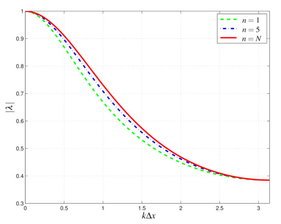
Figure 1. Implicit method: amplification factor module $\left|\lambda \right|$ for different values of n with $N=320$, $\mu =20$ and $x_{\infty }=1$.

In Figure 2, we show the amplification factor module for different values of $\mu$ at final time $\tau =T$. We observe that the unconditionally stable implicit finite difference scheme produces results that are stable for any value of the grid ratio $\mu$.

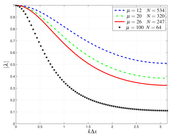
Figure 2. Implicit method: Amplification factor module $\left|\lambda \right|$ for different values of $\mu$ at time $\tau =T$. The implicit method results in stability for any value of $\mu$.

We can compare the result reported in Figure 2 with the results reported in Figure 3, where we show the amplification factor module $\lambda$, for different values of $\mu$, of the explicit method [20]

$$\begin{array}{ccc}\lambda \hfill & =& 1-r\Delta \tau -2\mu {\sigma }^2{sin}^2{\displaystyle \frac{k\Delta x}{2}}+i\mu \Delta x\left[\left(r-{\displaystyle \frac{{\sigma }^2}{2}}\right)+{\displaystyle \frac{1}{S_f^n}}{\displaystyle \frac{S_f^{n+1}-S_f^n}{\Delta \tau }}\right]sin(k\Delta x).\hfill \end{array}$$

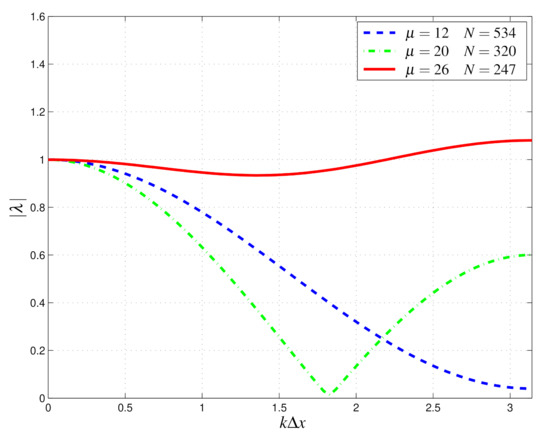
Figure 3. Explicit method: Amplification factor module $\left|\lambda \right|$ for different values of $\mu$ at time $\tau =T$. The explicit method becomes unstable for $\mu \ge 26$.

In order to evaluate $\lambda$, we use the same assumptions as for the implicit method. We observe that the explicit finite difference scheme produces results that are stable only for values of the grid ratio $\mu$ <26.

The main limitation of the explicit method is the restriction of the choice of $\Delta \tau$ and $\Delta x$, which have to be chosen in relation to the values of the parameters of the model $\sigma$ and r—the volatility of the underlying asset and the interest rate, respectively. On the other hand, the new implicit method is unconditionally stable, and thus no restriction on step sizes is required.

6. A Posteriori Error Estimator

In this section, we describe the a posteriori error estimator for the American put options problem based on Richardson’s extrapolation. In this way, we can find a more suitable computational grid requiring that the numerical solution obtained by the implicit method verifies a prefixed error tolerance.

For a scalar U of interest, either a value of the solution $p_j^n$ or a free boundary value $S_f^n$, the numerical error e can be defined by

$$e=u-U,$$

(24)

where u is the exact, usually unknown, value. When the numerical error is caused predominantly by the discretization error, in the case of smooth enough solutions, the global error can be split into a sum of powers of the inverse of N

$$u=U_N+C_0{\left(\frac{1}{N}\right)}^{q_0}+C_1{\left(\frac{1}{N}\right)}^{q_1}+C_2{\left(\frac{1}{N}\right)}^{q_2}+\cdots ,$$

(25)

where $C_0$, $C_1$, $C_2$, ⋯ are coefficients that depend on u and its derivatives but are independent of N, and $q_0$, $q_1$, $q_2$, ⋯ are the true orders of the discretization error; see Schneider and Marchi [27] and the references quoted therein. Each $q_k$ is usually a positive integer with $q_0<q_1<q_2<\cdots$ which together constitute an arithmetic progression of ratio $q_1-q_0$. The value of $q_0$ is called the asymptotic order or the order of accuracy of the method or of the numerical value $U_N$. By replacing $N=N_g$ and $N=N_{g+1}$ in Equation (25) and subtracting into the second obtained equation the first times ${(1/s)}^{q_0}$, where $s=N_{g+1}/N_g$, we get the first extrapolation formula

$$u\approx U_{g+1}+\frac{U_{g+1}-U_g}{s^{q_0}-1},$$

(26)

which has a leading order of accuracy equal to $q_1$. This type of extrapolation is due to Richardson [28,29]. Taking into account Equation (26), we can conclude that the error estimator using the first Richardson’s extrapolation is given by

$$e_r=\frac{U_{g+1}-U_g}{s^{q_0}-1},$$

(27)

where $q_0$ is the order of the numerical method used to compute the numerical solutions. Thus, (27) gives the real value of the numerical solution error without knowledge of the exact solution. In comparison with (27), a safer error estimator can be defined by

$$e_s=U_{g+1}-U_g.$$

(28)

Of course, $q_0$ can be estimated with the formula

$$q_0\approx \frac{log\left(\right|U_g-u\left|\right)-log\left(\right|U_{g+1}-u\left|\right)}{log\left(s\right)},$$

(29)

where u is again the exact solution (or, if the exact solution is unknown, a reference solution computed with a suitable large value of N) and both u and $U_{g+1}$ are evaluated at the same grid-points of $U_g$.

Within the above framework, in order to improve the numerical accuracy by using only a small number of grid-nodes, we can generalize (26) by introducing the following repeated extrapolation formula:

$$U_{g+1,k+1}=U_{g+1,k}+\frac{U_{g+1,k}-U_{g,k}}{s^{q_k}-1},$$

(30)

where $g\in \{0,1,2,\cdots ,G-1\}$, $k\in \{0,1,2,\cdots ,G-1\}$, $s=N_{g+1}/N_g$ is the grid refinement ratio, and $q_k$ is the true order of the discretization error. Formula (30) is asymptotically exact in the limit as $N_0$ goes to infinity if we use uniform grids. We notice that, to obtain each value of $U_{g+1,k+1}$, we need two computed solutions U in two adjacent grids, namely $g+1$ and g at the extrapolation level k. For any g, the level $k=0$ represents the numerical solution of U without any extrapolation. We recall that the theoretical orders of accuracy of the numerical values $U_{g,k}$, with $N=N_g$ and k extrapolations, verify the relation

$$q_k=q_0+k(q_1-q_0)$$

(31)

valid for $k\in \{0,1,2,\cdots ,G-1\}$.

7. Numerical Results

In this section, we show the numerical results obtained by using the implicit finite difference scheme. Comparisons with some numerical results available in the literature for the American put options problem are also presented. The numerical experiments were performed in MatLab on a computer equipped with a CPU Intel i7 under the operating system Windows 10.

The parameters considered for solving the American put option problem (3)–(6) are as follows:

$$r=0.1,\sigma =0.2,T=1.$$

(32)

In order to choose the truncated boundary value $x_{\infty }$, we compute the numerical solution $S_f^N$ for three different values of $x_{\infty }$. As we can see in Table 1, the change of these values does not greatly affect the numerical solution; for this reason, we decided to set $x_{\infty }=1$.

Table 1. Free boundary value $S_f^N$ at $\tau =T$ for different truncated boundary locations $x_{\infty }$.

${\mathit{x}}_{\mathit{\infty }}$	$\mathit{N}=10$	$\mathit{N}=20$	$\mathit{N}=40$
$0.7$	$0.8710513251234$	$0.8661003470130$	$0.86351373607045$
1	$0.8710513685210$	$0.8661003514438$	$0.86351373597835$
2	$0.8710513685385$	$0.8661003514444$	$0.86351373597828$
4	$0.8710513685388$	$0.8661003514438$	$0.86351373597789$

In Figure 4, we show the plots of $p_j^N$ versus $x_j$ and of $S_f^n$ versus ${\tau }^n$; these results were obtained by the implicit finite difference scheme, considering the parameters (32) with $N=320$ and $\mu =20$. We found the value $S_f^n=0.862718733223996$ in $15.536384$ seconds. In order to solve the non-linear system, we used the MATLAB routine “fsolve”. In general, the Newton iterations method represents a good tool in order to guarantee good computational stability properties. Initially, we used the classical Newton iteration method, but the obtained numerical results were less accurate when compared with those obtained by the MATLAB routine fsolve. By our numerical experiments, we conclude that the MATLAB routine, principally regarding the choice of the initial iterate, is more robust than the Newton iteration method and thus more suited for our application.

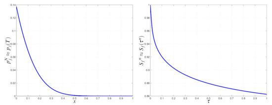
Figure 4. Numerical results obtained by the implicit scheme (8): on the left $p_j^N$ versus $x_j$, on the right, $S_f^n$ versus ${\tau }^n$, obtained with $J=80$, $N=320$ and $\mu =20$.

In Figure 5, the 3D plot of the numerical solution $p_j^n$ is shown.

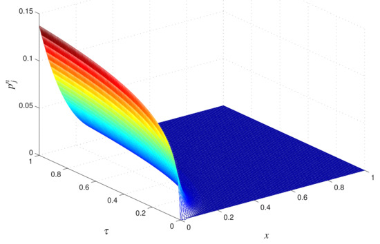
Figure 5. Numerical results obtained by implicit scheme (8), $p_j^n$ with $J=80$, $N=320$ and $\mu =20$.

Now, we consider the stability of the numerical method with respect to small perturbations of the starting parameters. In particular, we consider the perturbations $\delta r$ and $\delta \sigma$ related to the parameters involved in the model, namely r and $\sigma$. In Table 2, we show the numerical results obtained by different values of the perturbations. We can conclude that “small perturbations at input give rise to small perturbations at output”.

Table 2. Numerical results obtained by different perturbations.

$\mathit{\delta }\mathit{r}$	$\frac{|\mathit{\delta }{\mathit{S}}_{\mathit{f}}|}{\mathit{\delta }\mathit{r}}$	$\frac{|{\mathit{S}}_{\mathit{f}}^{\mathit{n}+1}+\mathit{\delta }{\mathit{S}}_{\mathit{f}}|}{\mathit{r}+\mathit{\delta }\mathit{r}}$	$\frac{|{\mathit{S}}_{\mathit{f}}^{\mathit{n}+1}+\mathit{\delta }{\mathit{S}}_{\mathit{f}}|}{|{\mathit{S}}_{\mathit{f}}^{\mathit{n}+1}|}$	$\frac{{\left|\right|\mathit{\delta }\mathit{p}\left|\right|}_{\mathit{\infty }}}{\mathit{\delta }\mathit{r}}$	$\frac{{\left|\right|\mathit{\delta }\mathit{p}\left|\right|}_{\mathit{\infty }}}{\mathit{r}+\mathit{\delta }\mathit{r}}$	$\frac{\left|\right|{\mathit{p}}^{\mathit{n}+1}+\mathit{\delta }\mathit{p}{\left|\right|}_{\mathit{\infty }}}{\left|\right|{\mathit{p}}^{\mathit{n}+1}{\left|\right|}_{\mathit{\infty }}}$
$\delta r=0.1$	0.740531	7.909584	1.008584	0.745939	1.181324	0.946084
$\delta r=0.05$	0.759815	8.251885	1.004403	0.765465	1.271923	0.972340
$\delta r=0.01$	0.776018	8.548762	1.000899	0.781872	1.352228	0.994350
$\mathbf{\delta }\mathbf{\sigma }$	$\frac{|\mathbf{\delta }{\mathbf{S}}_{\mathbf{f}}|}{\mathbf{\delta }\mathbf{\sigma }}$	$\frac{|{\mathbf{S}}_{\mathbf{f}}^{\mathbf{n}+\mathbf{1}}+\mathbf{\delta }{\mathbf{S}}_{\mathbf{f}}|}{\mathbf{\sigma }+\mathbf{\delta }\mathbf{\sigma }}$	$\frac{|{\mathbf{S}}_{\mathbf{f}}^{\mathbf{n}+\mathbf{1}}+\mathbf{\delta }{\mathbf{S}}_{\mathbf{f}}|}{|{\mathbf{S}}_{\mathbf{f}}^{\mathbf{n}+\mathbf{1}}|}$	$\frac{{\left|\right|\mathbf{\delta }\mathbf{p}\left|\right|}_{\infty }}{\mathbf{\delta }\mathbf{\sigma }}$	$\frac{\left|\right|{\mathbf{p}}^{\mathbf{n}+\mathbf{1}}+\mathbf{\delta }\mathbf{p}{\left|\right|}_{\infty }}{\mathbf{\sigma }+\mathbf{\delta }\mathbf{\sigma }}$	$\frac{\left|\right|{\mathbf{p}}^{\mathbf{n}+\mathbf{1}}+\mathbf{\delta }\mathbf{p}{\left|\right|}_{\infty }}{\left|\right|{\mathbf{p}}^{\mathbf{n}+\mathbf{1}}{\left|\right|}_{\infty }}$
$\delta \sigma =0.1$	1.013264	3.829016	0.9765080	1.025923	0.716437	1.147543
$\delta \sigma =0.05$	1.010532	4.059731	0.9882857	1.022231	0.702173	1.073572
$\delta \sigma =0.01$	1.007935	4.260559	0.9976631	1.018774	0.689935	1.014676

Looking at the results listed in Table 1, we realize also that, when fixing a value of the truncated boundary $x_{\infty }$, the computed values of $S_f^N$ for different values of the grid-steps are in agreement only up to the first decimal place. For this reason, we decide to improve the numerical accuracy by performing a mesh refinement and applying repeated Richardson’s extrapolation. The implicit difference scheme is accurate on the first order in time and second order in space; then, we can perform a mesh refinement keeping the grid ratio $\mu$ constant so that we end up with second-order truncation error $T_j^n=O(\Delta {\tau }^2)$ in time. Therefore, the global error is of the first order, which is the value of $q_0=1$. In our case, the sequence of $s^{q_k}$, for $k=0,1,\cdots$, with $s=4$ and $q_k=k+1$ is given by 4, 16, 64, 256, 1024, ⋯.

The numerical results obtained by repeated Richardson’s extrapolations for the values $S_f^N$ computed with the implicit method are reported in Table 3. The last extrapolated result is $U_{5,5}=0.862748$, so we can consider this value as our benchmark $S_f^N\approx 0.862748$. Our result can be compared with the value $S_f^N\approx 0.862762$ found by Fazio [21], with $S_f^N\approx 0.86222$ computed by Nielsen et al. [19] and with $S_f^N\approx 0.8628$ found by the explicit method of Company et al. [20].

Table 3. Implicit method: Richardson’s repeated extrapolations for the free boundary value $S_f^N$ at $\tau =T$.

N	${\mathit{U}}_{\mathit{g},0}$	${\mathit{U}}_{\mathit{g},1}$	${\mathit{U}}_{\mathit{g},2}$	${\mathit{U}}_{\mathit{g},3}$	${\mathit{U}}_{\mathit{g},4}$	${\mathit{U}}_{\mathit{g},5}$
5	$0.884069$
20	$0.866100$	$0.860111$
80	$0.863100$	$0.862100$	$0.862232$
320	$0.862719$	$0.862592$	$0.862625$	$0.862631$
1280	$0.862717$	$0.862716$	$0.862724$	$0.862726$	$0.862726$
5120	$0.862738$	$0.862746$	$0.862748$	$0.862748$	$0.862748$	$0.862748$

In Table 4, we compare the option price $P(S,T)$ obtained by different methods with the following parameters:

$$\begin{array}{c}T=3\sigma =0.2r=0.08E=100.\hfill \end{array}$$

(33)

Table 4. Comparison of American put option price $P(S,T)$ with parameters (33). PM: penalty method; EM: explicit method; EMR: explicit method with Richardson’s extrapolation; IM: implicit method; IMR: implicit method with Richardson’s extrapolation.

Asset	True	PM	EM	EMR	IM	IMR
Price S	Value	Nielsen [19]	Company [20]	Fazio [21]
90	$11.6974$	$11.7207$	$11.7054$	$11.7706$	$11.6926$	$11.7707$
100	$6.9320$	$6.9573$	$6.9309$	$6.9313$	$6.9243$	$6.9315$
110	$4.1550$	$4.1760$	$4.1564$	$4.1288$	$4.1467$	$4.1291$
120	$2.5102$	$2.5259$	$2.5151$	$2.5061$	$2.5028$	$2.5064$

We report the “true value” as in [30], the penalty method (PM) of Nielsen et al. given in [30], the explicit method (EM) of Company et al. [20] with $\Delta x=0.02$, the explicit method with Richardson’s extrapolation (EMR) of Fazio [21] with $\mu =5$ and our implicit method (IM) without extrapolation, setting $\Delta x=0.02$ and $\mu =5$, and with Richardson’s extrapolation (IMR) with $\mu =5$. In order to find the value of the option price $P(S,T)$ in correspondence to each different asset price S we use a piecewise cubic spline interpolation.

Our goal was to solve the American put option problem with a given tolerance $ϵ$, where 0 < $ϵ\ll$ 1; thus, we used the error estimator defined by Equation (27), or alternatively by Equation (28). To this end, we needed to solve the given problem twice, for two grids defined with given values of $J_g=J$ and $J_{g+1}=2J$ of space intervals but for the same value of the grid-ratio $\mu$. The corresponding time intervals $N_g$ and $N_{g+1}$ verify the relation $s=N_{g+1}/N_g$. Thus, we were able to apply (component-wise) to $p^n$ and to $S_f^n$ the error estimator in Formula (27) or (28). Then, we could verify whether, for $n=1,2,\cdots ,N$,

$$\parallel e_r\left(p^n\right){\parallel }_{\infty }\le ϵ\left|e_r\left(S_f^n\right)\right|\le ϵ.$$

(34)

If the two inequalities (34) hold true, for $n=1,2,\cdots ,N$, then we can accept the numerical solution computed on the grid defined by $J_{g+1}$ and $N_{g+1}$; otherwise, we have to increase these two integers and repeat the computation.

Figure 6 shows the error estimator results computed by setting $ϵ=0.005$. We set $\mu =20$ and start with $J_0=5$ and $J_1=10$ repeating the computation by doubling the number of spatial grid-intervals if the requi accuracy is not achieved. Our algorithm stops when $J_5=160$ that for $\mu =20$ means $N_5=1280$.

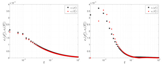
Figure 6. Numerical estimated errors $e_r\left(p^n\right)$ and $e_r\left(S_f^n\right)$ versus ${\tau }^n$ for the explicit (left) and implicit method (right), setting $ϵ=0.005$, $\mu =20$, $J_5=160$ and $N_5=1280$.

From the numerical results shown in Figure 6 we can easily see that the greatest errors are found within a few time steps for both numerical methods. The error of the implicit method is almost twice that of the error of the explicit scheme only in the first time steps, but it becomes smaller in the next time steps, so we can conclude that the numerical results obtained by the implicit method are more accurate than those of the explicit method. We suggest that in order to obtain better accuracy in the first time steps, an adaptive version of both finite difference schemes should be developed.

8. Concluding Remarks

In this paper, we consider an American put option model—a free boundary problem defined on an infinite domain. We overcome the numerical difficulty of solving a free boundary problem using a front-fixing approach combined with an implicit finite difference scheme. We prove that the implicit finite difference scheme is consistent and unconditionally stable. In order to improve the obtained accuracy, we use a mesh refinement and Richardson’s extrapolation technique. Comparisons with data available in the literature are carried out to validate the obtained numerical results. Finally, by using an a posteriori error estimator, we find a suitable computational grid that requires that the computed solution verifies a prefixed error tolerance.

References

- Black, F.; Scholes, M. The pricing of options and corporate liabilities. J. Polit. Econ. 1973, 81, 637–654. [Google Scholar] [CrossRef]
- Merton, R.C. The theory of rational option pricing. Bell J. Econ. Manag. Sci. 1973, 4, 141–183. [Google Scholar] [CrossRef]
- Schwartz, E.S. The valuation of warrants: Implementing a new approach. J. Financ. Econ. 1977, 4, 79–93. [Google Scholar] [CrossRef]
- Brennan, M.; Schwartz, E. The valuation of American put options. J. Financ. 1977, 32, 449–462. [Google Scholar] [CrossRef]
- Brennan, M.; Schwartz, E. Finite difference methods and jump processes arising in the pricing of contingent claims: A synthesis. J. Financ. Quant. Anal. 1978, 13, 461–474. [Google Scholar] [CrossRef]
- Jaillet, P.; Lamberton, D.; Lapeyre, B. Variational inequalities and the pricing of American options. Acta Appl. Math. 1990, 21, 263–289. [Google Scholar] [CrossRef]
- Hull, J.; White, A. Valuing derivative securities using the explicit finite difference method. J. Finac. Quant. Anal. 1990, 1, 87–100. [Google Scholar] [CrossRef]
- Duffy, D.J. Finite Difference Methods in Financial Engineering: A Partial Differential Equation Approach; John Wiley & Sons: Hoboken, NJ, USA, 2006. [Google Scholar]
- Wilmott, P.; Howison, S.; Dewynne, J. The Mathematics of Financial Derivatives; Cambridge University Press: Cambridge, UK, 1995. [Google Scholar]
- Han, H.; Wu, X. A fast numerical method for the Black–Scholes equation of American options. SIAM J. Numer. Anal. 2003, 41, 2081–2095. [Google Scholar] [CrossRef]
- Pantazopoulos, K.N.; Houstis, E.N.; Kortesis, S. Front-tracking finite difference methods for the valuation of American options. Comput. Econ. 1998, 12, 255–273. [Google Scholar] [CrossRef]
- Tangman, D.Y.; Gopaul, A.; Bhuruth, M. A fast high-order finite difference algorithm for pricing American options. J. Comput. Appl. Math. 2008, 222, 17–29. [Google Scholar] [CrossRef]
- Holmes, A.D.; Yang, H. A front-fixing finite element method for the valuation of American options. SIAM J. Sci. Comput. 2008, 30, 2158–2180. [Google Scholar] [CrossRef]
- Wu, L.; Kwok, Y.-K. A front-fixing method for the valuation of American option. J. Financ. Eng. 1997, 6, 83–97. [Google Scholar]
- Zhu, Y.L.; Chen, B.M.; Ren, H.; Xu, H. Application of the singularity separating method to American exotic option pricing. Adv. Comput. Math. 2003, 19, 147–158. [Google Scholar] [CrossRef]
- Ševčovič, D. An iterative algorithm for evaluating approximations to the optimal exercise boundary for a nonlinear Black–Scholes equation. Can. Appl. Math. Q. 2007, 15, 77–97. [Google Scholar]
- Lauko, M.; Ševčovič, D. Comparison of numerical and analytical approximations of the early exercise boundary of American put options. ANZIAM J. 2010, 51, 430–448. [Google Scholar] [CrossRef][Green Version]
- Zhang, J.; Zhu, S.P. A hybrid finite difference method for valuing American puts. In Proceedings of the World Congress on Engineering 2009, London, UK, 1–3 July 2009; Ao, S.I., Gelman, L., Hukins, D.W.L., Hunter, A., Korsunsky, A.M., Eds.; IAENG: Kwun Tong, Hong Kong, 2009; Volume II, pp. 1131–1136. [Google Scholar]
- Nielsen, B.F.; Skavhaug, O.; Tveito, A. Penalty and front-fixing methods for the numerical solution of American option problems. J. Comput. Financ. 2002, 5, 69–97. [Google Scholar] [CrossRef]
- Company, R.; Egorova, V.N.; Jódar, L. Solving American option pricing models by the front fixing method: Numerical analysis and computing. Abstr. Appl. Anal. 2014, 2014, 146745. [Google Scholar] [CrossRef]
- Fazio, R. A posteriori error estimator for a front-fixing finite difference scheme for American options. In Proceedings of the World Congress on Engineering 2015, London, UK, 1–3 July 2015; Ao, S.I., Gelman, L., Hukins, D.W.L., Hunter, A., Korsunsky, A.M., Eds.; IAENG: Kwun Tong, Hong Kong, 2015; Volume II, pp. 691–696. [Google Scholar]
- Fazio, R. American put option: Richardson’s extrapolation and a posteriori error estimator for a front-fixing finite difference scheme. Appl. Math. E Notes 2020, 20, 445–457. [Google Scholar]
- Fazio, R.; Insana, A.; Jannelli, A. Front fixing finite difference schemes for American put options model. In Proceedings of the International Conference of Numerical Analysis and Applied Mathematics (ICNAAM2015), Rhodes, Greece, 22–28 September 2016. [Google Scholar]
- Kangro, R.; Nicolaides, R. Far field boundary conditions for Black–Scholes equations. SIAM J. Numer. Anal. 2000, 38, 1357–1368. [Google Scholar] [CrossRef]
- Kwok, Y.-K. Mathematical Models of Financial Derivatives, 2nd ed.; Springer: Berlin/Heidelberg, Germany, 2008. [Google Scholar]
- Aslak, T.; Ragnar, W. Introduction to Partial Differential Equations: A Computational Approach; Sringer: New York, NY, USA, 1998. [Google Scholar]
- Schneider, F.A.; Marchi, C.H. On the grid refinement ratio for one-dimensional advection problems with nonuniform grids. In Proceedings of the 18th International Congress of Mechamical Engineering (COBEM 2005), Ouro Preto, MG, USA, 6–11 November 2005; p. 8. [Google Scholar]
- Richardson, L.F. The approximate arithmetical solution by finite differences of physical problems involving differential equations, with an application to the stresses in a masonry dam. Proc. R. Soc. Lond. Ser. A 1910, 210, 307–357. [Google Scholar]
- Richardson, L.F.; Gaunt, J.A. The defer approach to the limit. Proc. R. Soc. Lond. Ser. A 1927, 226, 299–349. [Google Scholar]
- Saib, F.A.A.E.; Tangman, Y.D.; Thakoor, N.; Bhuruth, M. On some finite difference algorithms for pricing American options and their implementation in mathematica. In Proceedings of the 11th International Conference on Computational and Mathematical Methods in Science and Engineering (CMMSE ’11), Alicante, Spain, 26–30 June 2011. [Google Scholar]
Publisher’s Note: MDPI stays neutral with regard to jurisdictional claims in published maps and institutional affiliations. |
© 2021 by the authors. Licensee MDPI, Basel, Switzerland. This article is an open access article distributed under the terms and conditions of the Creative Commons Attribution (CC BY) license (https://creativecommons.org/licenses/by/4.0/).