Abstract
The COVID-19 disease constitutes a global health contingency. This disease has left millions people infected, and its spread has dramatically increased. This study proposes a new method based on a Convolutional Neural Network (CNN) and temporal Component Transformation (CT) called CNN–CT. This method is applied to confirmed cases of COVID-19 in the United States, Mexico, Brazil, and Colombia. The CT changes daily predictions and observations to weekly components and vice versa. In addition, CNN–CT adjusts the predictions made by CNN using AutoRegressive Integrated Moving Average (ARIMA) and Exponential Smoothing (ES) methods. This combination of strategies provides better predictions than most of the individual methods by themselves. In this paper, we present the mathematical formulation for this strategy. Our experiments encompass the fine-tuning of the parameters of the algorithms. We compared the best hybrid methods obtained with CNN–CT versus the individual CNN, Long Short-Term Memory (LSTM), ARIMA, and ES methods. Our results show that our hybrid method surpasses the performance of LSTM, and that it consistently achieves competitive results in terms of the MAPE metric, as opposed to the individual CNN and ARIMA methods, whose performance varies largely for different scenarios.
1. Introduction
Coronaviruses are a large family of viruses characterized by having crown-shaped spikes on their surface. Nowadays, there are seven identified types of coronaviruses that can be transmitted among humans. The most dangerous coronaviruses known until recent years are MERS-CoV and SARS-CoV, and they have caused severe diseases, such as MERS and SARS, in 2003 and 2012, respectively, [1]. However, at the end of 2019, in Wuhan, China, the new epidemiological outbreak of COVID-19 emerged; it was caused by the new coronavirus called SARS-CoV2.
The importance of mathematical models and algorithms to analyze this disease has grown because they allow one to find patterns, make predictions, and understand fluctuations. Epidemiological models can be classified into two groups [2]:
- Dynamic Models. These are old models that usually divide the population into several subsets known as compartments, for instance, the Susceptible, Infectious, Recovered or SIR model. The SIR model was proposed in 1902 by Sir Roland Ross and then expanded by Kermack and McKendrick in 1927 [3].
- Forecasting models using time series. Here, we find classical methods such as ARIMA and Exponential Smoothing (ES) [4]. Furthermore, Machine Learning methods like Support Vector Machines [5] and Deep Learning [6] are also in this group.
This work presents a new method of the second group, based on Convolutional Neural Network (CNN) [7] and a proposed Component Transformation (CT), which we named CNN–CT, whose mathematical formulation is presented. The CNN–CT method is applied to forecast the number of COVID-19 confirmed cases for the United States (US), Mexico, Brazil, and Colombia [8]. The CT changes daily observations into weekly data and back. The forecast made by our hybrid CNN–CT method is further adjusted either with ARIMA or ES methods. We compared the proposed hybrid method versus the individual methods. Our results show that the combined method consistently achieves competitive results in terms of the MAPE metric, as opposed to any of its elements—CNN, ARIMA, or ES—whose performance as individual methods varies largely for different countries. Moreover, the proposed CNN–CT method also outperforms the Long Short-Term Memory (LSTM) [9], which is among the most used methods for dealing with time-series.
Both CNN and LSTM are Deep Learning methods, the first of which is equipped with convolutional filters while the second with recurrent operations, but in both cases with parameters that are learned though gradient-descent-like methods in a scenarios where data are used for training as they become available. In contrast, ARIMA and ES are traditional regression methods that consider a full set of training data at once, thus having the potential of better approximating such a training set, but losing the ability to adjust to newly available data as CNN and LSTM can. The proposed CNN–CT method exploits both the potential of incorporating newly available data as well as the strength of looking at a complete set at once, which results in an enriched forecast method.
We chose to use CNNs, given that the signal processing literature states that convolutional filters are more stable than recurrent operations like LSTM [10]. Moreover, the superior performance of CNNs over traditional methods, like ARIMA, has been confirmed by previous work focused on text classification [11] and sequence modeling [12], where convolutions obtained higher performance with respect to other methods.
The rest of this paper is organized as follows. In Section 2, we discuss works related to the forecast of confirmed cases of COVID-19. In Section 3, we show the proposed forecasting method for daily confirmed cases of COVID-19, highlighting the application of Deep Learning, ARIMA, and ES methods. In Section 4, we present details about the data and tools used to validate our method. Finally, Section 5 and Section 6 present results and conclusions of this work.
2. Related Works
COVID-19 is a disease with a high rate of spread, which has led to an interest in estimation and forecasting the number of cases of infected people. Recently, several works have been presented with traditional epidemiological models or Dynamic Models. The Susceptible, Exposed, Infectious, Recovered (SEIR) model [13] was used to forecast confirmed cases in the United Kingdom, and the SIR and SEIR models were applied to forecast cumulative infected and recovered cases in Santiago de Cuba [14]. The Susceptible, Exposed, Infectious, Recovered, Dead (SEIRD) model [15] was used to forecast confirmed and death cases in Mexico. At Chen [16], comparative work was conducted to predict 11 days of confirmed cases in some regions of Canada and the United States. They use SIR, Neural Network, and ARIMA models.
The ARIMA and ES were used as adjusting methods to improve the results obtained for other models such as those obtained for SIR models, Neural Networks, and Support Vector Regression algorithms [2,17]. However, in most cases, the number of days forecast is too short. For instance, the authors of [18] used ARMA to forecast confirmed cases for three days in Chinese provinces, Asian countries, and a few occidental countries (Germany, US, Italy, and Spain). Parvez et al. compared an Adaptive Neuro-fuzzy Inference System versus ARIMA to predict ten days of COVID-19 confirmed cases in Bangladesh [19]. Furthermore, Petropoulus et al. [20], used the ES method known as Holt-Winter to forecast ten days of globally accumulated COVID-19 confirmed cases. Hussain et al. [21], used an ES to estimate twelve days of confirmed cases, and the parameter known as the basic reproduction number.
ARIMA and Deep Learning methods have been used alone to forecast COVID-19 cases. Chimmula [22] used LSTM to predict daily cases, obtaining with this method an error of eight percent using MAPE. In Chandraa [23], LSTM, BiLSTM, and EDLSTM were used to forecast the spread of COVID-19 infections among selected states in India. The work presented by Zeroul et al. [24] used deep learning to predict 10 days of number of infected people, obtaining a MAPE error between and . Saba et al. [25] compared polynomial regression, Holt-Winter, ARIMA, and SARIMA models, to predict the confirmed and deaths cases. Parbat et al. [26] proposed using an SVR-Radial model to forecast total deaths and recovered, daily confirmed cumulative, and confirmed daily deaths in India; this method obtained around thirteen percent MAPE error for the entire country.
Moreover, classical forecast methods have been combined with Machine Learning techniques [2,17,27]. Katris [27] used ARIMA, ES, Neural Network, and MARS models, where the combined methods performed better than the individual methods.
In general, ARIMA and ES methods are used to forecast cases with short-term periods, while Machine Learning and Deep Learning models are able to predict cases over more extended periods. However, the latter do not always obtain good results when used as individual methods.
3. CNN–CT Method
We show the proposed CNN–CT method in Figure 1, where a Convolutional Neural Network is used as primary forecasting method for daily confirmed cases of COVID-19, and it is complemented by ARIMA or ES, which are used as adjusting methods against daily errors.
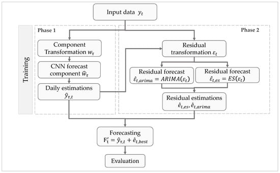
Figure 1.
Proposed Convolutional Neural Network (CNN) and temporal Component Transformation (CT) (CNN–CT ) method. Training with two phases: the first phase corresponds to forecast method using component values, and the second phase used residual values with a residual forecast method.
Firstly, our method’s training stage is composed of two phases, each of which is formed by three internal sub-processes plus one global integration sub-process, as is shown in Figure 1.
In the first sub-process of phase 1, we start by transforming daily values into weekly components , where t is a day index and is a component index. These components represent average weekly forecast estimations. In the second sub-process, a CNN is used to forecast the component . Finally, in the third sub-process, we convert the component estimation back into daily estimations .
In phase 2, the adjusting methods are trained. First, we obtain the residual from the difference between the daily prediction and its corresponding ground truth value, i.e., . We scale these residual values to be in the range , as required by the Holt-Winter methods.
In the second sub-process of phase 2, we use the residuals to train an autoregressive model using either ARIMA or ES, which is used to forecast residual values (concretely, and for ES and ARIMA, respectively).
Later, in the third sub-process of phase 2, residual forecasts or are obtained from the previously computed residual forecast values. Finally, this residual forecast is added to the daily estimation obtained from the CNN, resulting in the final prediction value .
3.1. Data Transformation
Prediction models reflect an increased error as the number of forecasting periods increases. We chose to forecast more cases by transforming daily records into weekly components with the CT module, which maps the daily cases into components that represent a weighted average of the daily cases obtained within a week. The values are calculated with Equation (1).
where is the weekly average of week and is a set of transformed observation into components. For instance, .
3.2. CNN Forecast Component
We used a CNN as a component forecasting method. The training and validation stages are composed of values. The CNN architecture contains an input layer with 50 convolutional neurons, a maxpooling layer of size equals 2. A complete MLP layer of 50 neurons, and one output layer with a single neuron. The convolutional layers use the ReLU activation function. The training configuration parameters is as follows: Adam optimizer [28], mean absolute error as loss function, 100 epochs, and batch size equal to 10. The above configuration is used to forecast weekly components .
3.3. Daily Estimations
The reverse transformation or daily estimations involves converting the weekly components back into daily values. For this, it is necessary to calculate the subcomponents of a component, which we define as shown in Table 1.

Table 1.
Component segmentation into subcomponents.
The segmentation of the week into two subcomponents provides insights about the social behavior of countries separately into beginning and end of a week. The distribution of the daily cases with respect to their subcomponents can be obtained by Equations (2) and (3).
where are subcomponents ADS-1 (Monday to Thursday) and ADS-2 (Friday to Sunday) for the component . We determine that the daily ratio represents the proportion of the original daily values for subcomponent 1 and 2 for the component (Equation (4)). The daily ratio lets us to determine weekday normalized cases (Equation (5)) of the training phase. In other words, are average confirmed cases of each day of the week throughout the time series.
The weighting of the daily cases obtained with the ratio allows obtaining a statistical estimation on the relevance of persons infected in the first and second subcomponent of each component throughout the training period. The inverse transformation determines the daily cases predicted from the components using Equations (6) and (7).
where represents the forecasting case values of the component at time t, and is the forecast of the average number of infected sub-component i in the component. The data for the learning of the adjustment methods are obtained from the daily prediction values of the validation phase of components .
3.4. Residual Transformation
A residual value is given by the difference in the ground truth and the predicted value, as shown in Equation (8).
where is the ground truth in time t, is the forecast value in time t. Using Equation (8), the residuals are obtained by subtraction of and , as shown in Equation (9).
where is the forecasting value in time t of component . ARIMA and ES methods used positive numbers; because of this, the residuals were normalized as shown in Equation (10).
where represents normalization of in the range of values .
3.5. Residual Forecast
We used ARIMA and ES forecasting methods as forecasting adjustments methods. The training and validation sets are composed by values.
The configuration of the ARIMA method is as follows: start_p = 0, d = 0, start_q = 0, max_p = 5, max_q = 5, max_d = 5, start_Q = 0, max_P = 5, max_D = 5, max_Q = 5, m = 4, seasonal = True, error_action = ‘warn’, trace = True, suppress_warnings = True, stepwise = True, random_state = 20, n_fits = 50, information_criterion = ‘aic’, and alpha = 0.05.
Furthermore, ES obtained a configuration that used the Holt–Winter (HW) method. The variants of HW used are: additive, multiplicative, additive damped, multiplicative damped. These variants were trained with a norm residuals .
3.6. Residual Estimations
We use residual transformations to train ARIMA and ES, from which we obtained four hybrid methods, CNN-ARIMA, CNN-ES, LSTM-ARIMA, and LSTM-ES. The forecasts and from these hybrid methods are transformed into residuals , which are in the non-normalized domain.
3.7. Forecasting
Finally, we evaluated the forecast values of the validation phase , which is composed of the daily forecasts of CNN and adjustment forecasts , as is shown in Equation (11).
4. Experimental Setup
The source of the data, the pre-processing applied, the data separation criterion in training, validation, and testing are described below. Finally, the evaluation metrics are described.
4.1. Data
The COVID-19 database used in this work is the Novel Coronavirus 2019 dataset [8], whose records report the number of infected, recovered, and deceased people in each country of the world. From this database, we used a time series starting from 22 January 2020, and that is called Time_Series_Covid_19_confirmed. We selected the records corresponding to the US, Mexico, Brazil, and Colombia.
We used data records from 2 March 2020 until 28 June 2020 for training (17 weeks); from 29 June 2020 to 19 July 2020 for validation (3 weeks); and from 20 July 2020 to 9 August 2020 for test (3 weeks). Figure 2 shows a scheme for this split of data.
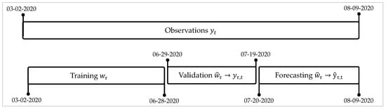
Figure 2.
Split of the observations in training and validation set by CNN method.
With this split, the training of the CNN–CT method for the US was carried out with 17 weekly components , as explained in Section 3.1. In the case of Mexico, Brazil, and Colombia, we used only 15 weekly components since the data corresponding to the first week were discarded due to the lack of significant information; that is, the values of the first week were considerably low with respect to the rest of the series. We noticed that processing this first week results in underestimation of the forecast values.
Although training is conducted using weekly components , the forecast for the validation and test stages happens in daily values , as explained in Section 3.3.
Residual forecasts allow adjusting daily forecast with ARIMA and ES. In addition, it trained with the residuals of forecast daily validation means, and forecasts obtained in the validation phase were transformed into daily estimations to be used in the training and validation phase of the adjustment methods. Figure 3 shows a scheme for this split of data for the adjusting methods.
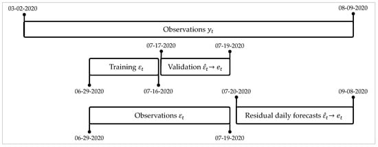
Figure 3.
Split of the observations in training and validation set by adjusting methods.
Given that the problem we address corresponds to a scenario of auto-regression, the actual structure of the data is such that each output variable depends on a vector of past values . For this work, we used lags of up to three past values, , , and .
4.2. Metrics
The proposed hybridized CNN–CT method and its individual composing methods are evaluated by the MAPE [29], as it has been widely used in the works discussed in Section 2. The MAPE computes the percentage of accuracy in the predicted value with respect to the ground truth. The closer to zero, the more accurate it is. Another common metric is RMSPE [4] which is also used in part of this paper.
where, is the ground truth, is the predicted value, and n indicates the total number of samples.
4.3. Tools
This work was developed with a computer with an iOS operating system, 8 GB, and a 2.3 GHz Dual-Core Intel Core i5 processor. We used Python 3.7.1, and the CNN model was built using Tensorflow and Keras libraries [30].
5. Results
This section shows the results of the CNN–CT method proposed for daily forecasting cases of COVID-19 in the US, Mexico, Brazil, and Colombia. First, we compare the performance of using CNN and LSTM as the main forecasting methods with ARIMA and ES (Holt-Winter, HW) as adjusting methods. Then, we present the comparison of the CNN–CT model versus the individual CNN, LSTM, ARIMA, and Holt-Winters models for each country.
We can see in Figure 4 the comparison of best-performing forecast models for the countries of The United States, Mexico, Brazil, and Colombia. In the US, Figure 4a, the forecasts of LSTM-ARIMA manage to maintain the trend and seasonality patterns with respect to the ground truth. However, the CNN-HW prognosis is well below the actual data. We can see in Table 2 that LSTM-ARIMA achieves the lowest MAPE for the US.
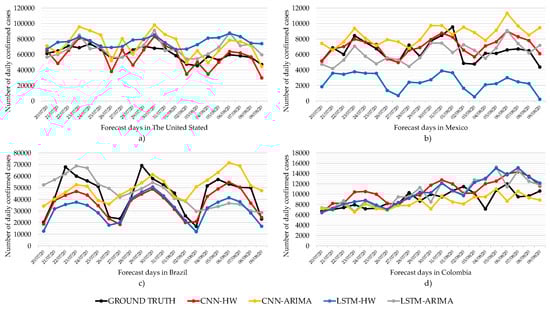
Figure 4.
Daily forecast with CNN–CT method using CNN and Long Short-Term Memory (LSTM) as main forecast methods.
Table 2.
CNN–CT methods performance. Best MAPE results are marked in bold.
Likewise, Figure 4b shows the behavior of the forecasts for daily cases of COVID-19 in Mexico. We can see that all four models are able to maintain trend and seasonality patterns with respect to ground truth. However, LSTM–ARIMA shows a high error rate because of the difference with respect to the actual data. On the other hand, the forecast of CNN-HW is very close to the real data, which allows us to obtain a better performance with respect to the other methods. The average MAPE and its standard deviation are shown in Table 2, where we can see that CNN-HW achieves the best average performance among the four models.
Similarly, Figure 4c shows the comparative Brazil forecast for all the models. We can see that LSTM-ARIMA manages to maintain seasonality patterns concerning the ground truth. In the case of CNN-HW, it follows the trend and seasonality patterns with respect to the ground truth. The average MAPE and its standard deviation are shown in Table 2. However, as we noticed before with the average MAPE and its standard deviation, CNN–HW has the best performance.
We can see in Figure 4d that LSTM–ARIMA manages to maintain seasonality patterns concerning the ground truth for Colombia. In the case of CNN–HW, it follows the trend and seasonality patterns concerning the ground truth. According to Table 2 CNN-ARIMA shows the best MAPE performance, as its curve is the closest to the ground truth.
In general, our experiments show that smoothing with ARIMA or ES helps obtain lower MAPE in the case of CNN. This is not the case with LSTM. Table 2 shows a summary of the MAPE and RMSPE daily forecasting values of the CNN–CT and LSTM–CT for US, Mexico, Brazil, and Colombia. In the case of US, the method with the best performance is LSTM-ARIMA, having a . In the case of Mexico and Brazil, CNN–HW is better with MAPE and . It is possible to see that LSTM–ARIMA and CNN–HW obtain better results in different countries. In Colombia, CNN-ARIMA obtains the best MAPE and RMSPE.
We averaged the MAPE of all the countries for each method in Table 2. We observed that CNN–CT methods have better performance than that of LSTM–CT. Furthermore, for each country, we determined the standard deviation of the error metrics. We noticed that CNN–CT has the lower deviation, which indicates that its best performance is consistent across countries.
Finally, in Figure 5, we show a comparison of the MAPE for the CNN-HW model versus the individual CNN, LSTM, ARIMA, and Holt–Winters models for each country.
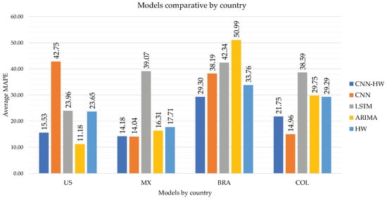
Figure 5.
Daily forecast with CNN–CT (using Holt–Winters (HW)) versus the individual methods CNN, LSTM, ARIMA, and HW.
Although ARIMA obtained good performance for the US (11.18) and Mexico (16.31), first and third place, respectively, it provides high MAPE for Brazil (50.99) and Colombia (29.75), with the last and second-last places, respectively. Similarly, pure CNN is a good method for Mexico (14.04) and Colombia (14.96) but not so good for US (42.75) and Brazil (38.19).
In contrast, CNN–CT (CNN-HW) is consistently competitive for all cases, obtaining second place for US (15.53), Mexico (14.18, as good as the best-performing CNN alone), and Colombia (21.75), and first for Brazil (29.30).
We show the comparison of CNN–HW versus the four individual methods in Table 3. We can see that CNN–HW surpasses all of these individual methods for Brazil and Colombia. For the case of Mexico, CNN–HW is below the best performing method (CNN) only by 0.14 MAPE points. Furthermore, CNN–HW achieves competitive results for the US.
Table 3.
The performance of the CNN–CT vs. individual methods. Best MAPE results are marked in bold.
6. Conclusions
This paper investigates the problem of forecasting confirmed daily cases of COVID-19 in Mexico, Brazil, Colombia, and the US. Given the limited number of data available at the time of conducting our experiments, several limitations of the prediction methods became evident. These limitations were even more obvious due to the presence of noise in the daily data, which might very well be a consequence of the restrictions on the flow of data imposed by the sanitary crisis related to COVID-19 worldwide.
In particular, most prediction methods decrease their accuracy as the periods for forecast become larger. To mitigate this issue, we proposed a component transformation that converts daily values into weekly components for correct prediction in those cases.
We present a hybrid forecasting method termed Convolutional Neural Network–Component Transformation (CNN–CT), which uses CNN and LSTM as the main prediction method and ES and ARIMA as adjusting methods for daily error correction. As a result, there are two variants of the proposed method: CNN–CT with Holt–Winters, and LSTM–CT with ARIMA.
We compared the prediction performance of the individual methods that compose the proposed CNN–CT using the MAPE metric. We noticed that CNN and LSTM are very good with learning trend and seasonality of the time series; however, LSTM forecasts tends to generate increasing and decreasing trend, which causes the error to increase. Our experiments show that smoothing with ARIMA or ES helps obtain lower MAPE in the case of CNN. This is not the case with LSTM.
As future works, we propose applying this methodology to other popular forecasting methods such as SVR, Recurrent Neural Network, and so on; measuring the performance quality in more countries; and applying powerful data cleaning as a preprocessing stage. Furthermore, it could be interesting to use different adjusting methods. Finally, we propose testing if the proposed methodology is completely general or determines which strategy applies in different forecast scenarios.
Author Contributions
Conceptualization L.J.H.-G., J.F.-S., and J.J.G.-B.; methodology L.J.H.-G., J.F.-S., E.R.-R., and J.J.G.-B.; investigation L.J.H.-G., J.F.-S., and J.J.G.-B.; Software L.J.H.-G., J.F.-S., and J.J.G.-B.; validation, J.F.-S., J.P.S.-H., and E.R.-R.; formal analysis J.F.-S., J.P.S.-H., and E.R.-R.; writing—original draft L.J.H.-G. and J.F.-S.; writing—review and editing, J.F.-S., J.J.G.-B., E.R.-R., and J.P.S.-H. All authors have read and agreed to the published version of the manuscript.
Funding
This research received no external funding.
Acknowledgments
The authors would like to acknowledge with appreciation and gratitude CONACYT, TecNM/Instituto Tecnológico de Ciudad Madero, and Asociación Maxicana de Cultura A.C. In addition, the authors acknowledge the support from Laboratorio Nacional de Tecnologías de la Información (LaNTI) for the access to the cluster.
Conflicts of Interest
The authors declare no conflict of interest.
References
- Sahu, K.K.; Mishra, A.K.; Lal, A. Coronavirus disease-2019: An update on third coronavirus outbreak of 21st century. QJM Int. J. Med. 2020, 113, 384–386. [Google Scholar] [CrossRef]
- Frausto Solis, J.; Olvera Vazquez, J.E.; González-Barbosa, J.J. The Hybrid Forecasting Method SVR-ESAR for COVID-19 Background. Int. J. Comb. Optim. Probl. Inform. 2021, 12, 42–48. [Google Scholar]
- Kermack, W.O.; McKendrick, A.G. A contribution to the mathematical theory of epidemics. Proc. R. Soc. Lond. Ser. A Contain. Pap. A Math. Phys. Character 1927, 115, 700–721. [Google Scholar] [CrossRef]
- Hyndman, R.J.; Athanasopoulos, G. Forecasting: Principles and Practice; Monash University: Melbourne, Australia, 2018. [Google Scholar]
- Cortes, C.; Vapnik, V. Support-vector networks. Mach. Learn. 1995, 20, 273–297. [Google Scholar] [CrossRef]
- Goodfellow, I.; Bengio, Y.; Courville, A. Deep Learning; MIT Press: Cambridge, MA, USA, 2016; Volume 1, p. 692. [Google Scholar]
- LeCun, Y.; Bengio, Y. Convolutional networks for images, speech, and time series. Handb. Brain Theory Neural Netw. 1995, 3361, 255–258. [Google Scholar]
- SRK. Novel CoronaVirus 2019 Dataset; Kaggle: San Francisco, CA, USA, 2020. [Google Scholar]
- Hochreiter, S.; Schmidhuber, J. Long short-term memory. Neural Comput. 1997, 8, 1735–1780. [Google Scholar] [CrossRef]
- Roberts, M.J. Signals and Systems: Analysis Using Transform Methods and MATLAB, 3rd ed.; McGraw-Hill: New York, NY, USA, 2018. [Google Scholar]
- Zhang, X.; Zhao, J.; LeCun, Y. Character-level Convolutional Networks for Text Classification. In Proceedings of the Advances in Neural Information Processing Systems: Annual Conference on Neural Information Processing Systems 2015, Montreal, QC, Canada, 7–12 December 2015. [Google Scholar]
- Bai, S.; Kolter, J.Z.; Koltun, V. An Empirical Evaluation of Generic Convolutional and Recurrent Networks for Sequence Modeling. arXiv 2018, arXiv:1803.01271. [Google Scholar]
- Keeling, M.J.; Hill, E.M.; Gorsich, E.E.; Penman, B.; Guyver-Fletcher, G.; Holmes, A.; Leng, T.; McKimm, H.; Tamborrino, M.; Dyson, L.; et al. Predictions of COVID-19 dynamics in the UK: Short-term forecasting and analysis of potential exit strategies. PLoS Comput. Biol. 2021, 17, e1008619. [Google Scholar] [CrossRef] [PubMed]
- Ramirez-Torres, E.E.; Selva Castañeda, A.R.; Rodríguez-Aldana, Y.; Sánchez Domínguez, S.; Valdés García, L.E.; Palú-Orozco, A.; Oliveros-Domínguez, E.; Zamora-Matamoros, L.; Labrada-Claro, R.; Cobas-Batista, M.; et al. Mathematical modeling and forecasting of COVID-19: Experience in Santiago de Cuba province. Rev. Mex. Física 2021, 67, 123. [Google Scholar] [CrossRef]
- Capistran, M.A.; Capella, A.; Christen, J.A. Forecasting hospital demand in metropolitan areas during the current COVID-19 pandemic and estimates of lockdown-induced 2nd waves. PLoS ONE 2021, 16, e0245669. [Google Scholar] [CrossRef]
- Chen, L.P.; Zhang, Q.; Yi, G.Y.; He, W. Model-based forecasting for Canadian COVID-19 data. PLoS ONE 2021, 16, e0244536. [Google Scholar] [CrossRef]
- Ala’raj, M.; Majdalawieh, M.; Nizamuddin, N. Modeling and forecasting of COVID-19 using a hybrid dynamic model based on SEIRD with ARIMA corrections. Infect. Dis. Model. 2021, 6, 98–111. [Google Scholar] [CrossRef]
- Deb, S.; Majumdar, M. A time series method to analyze incidence pattern and estimate reproduction number of COVID-19. arXiv 2020, arXiv:abs/2003.10655. [Google Scholar]
- Parvez, S.M.; Rakin, S.S.A.; Asadut Zaman, M.; Ahmed, I.; Alif, R.A.; Rahman, R.M. A Comparison Between Adaptive Neuro-fuzzy Inference System and Autoregressive Integrated Moving Average in Predicting COVID-19 Confirmed Cases in Bangladesh. ICT Anal. Appl. 2021, 154, 741–754. [Google Scholar] [CrossRef]
- Petropoulos, F.; Makridakis, S. Forecasting the novel coronavirus COVID-19. PLoS ONE 2020, 15, e0231236. [Google Scholar] [CrossRef]
- Hussain, Z.; Dutta Borah, M. Forecasting Probable Spread Estimation of COVID-19 Using Exponential Smoothing Technique and Basic Reproduction Number in Indian Context; Springer: Berlin/Heidelberg, Germany, 2021; pp. 183–196. [Google Scholar] [CrossRef]
- Chimmula, V.K.R.; Zhang, L. Time series forecasting of COVID-19 transmission in Canada using LSTM networks. Chaos Solitons Fractals 2020, 135, 109864. [Google Scholar] [CrossRef]
- Chandraa, R.; Jainb, A.; Chauhanc, D.S. Deep learning via LSTM models for COVID-19 infection forecasting in India. arXiv 2021, arXiv:2101.11881. [Google Scholar]
- Zeroual, A.; Harrou, F.; Dairi, A.; Sun, Y. Deep learning methods for forecasting COVID-19 time-series data: A comparative study. Chaos Solitons Fractals 2020, 140. [Google Scholar] [CrossRef] [PubMed]
- Saba, T.; Abunadi, I.; Shahzad, M.N.; Khan, A.R. Machine learning techniques to detect and forecast the daily total COVID-19 infected and deaths cases under different lockdown types. Microsc. Res. Tech. 2021, jemt.23702. [Google Scholar] [CrossRef] [PubMed]
- Parbat, D.; Chakraborty, M. A python based support vector regression model for prediction of COVID19 cases in India. Chaos Solitons Fractals 2020, 138, 3–7. [Google Scholar] [CrossRef]
- Katris, C. A time series-based statistical approach for outbreak spread forecasting: Application of COVID-19 in Greece. Expert Syst. Appl. 2021, 166, 114077. [Google Scholar] [CrossRef]
- Kingma, D.P.; Ba, J. Adam: A Method for Stochastic Optimization. In Proceedings of the 3rd International Conference on Learning Representations, ICLR, San Diego, CA, USA, 7–9 May 2015. [Google Scholar]
- Makridakis, S.; Armstrong, J.S.; Carbone, R.; Fildes, R. An editorial statement. J. Forecast. 1982, 1, 1–2. [Google Scholar] [CrossRef]
- Raschka, S.; Mirjalili, V. Python Machine Learning: Machine Learning and Deep Learning with Python, Scikit-Learn, and TensorFlow, 2nd ed.; Packt Publishing: Birmingham, UK, 2017. [Google Scholar]
Publisher’s Note: MDPI stays neutral with regard to jurisdictional claims in published maps and institutional affiliations. |
© 2021 by the authors. Licensee MDPI, Basel, Switzerland. This article is an open access article distributed under the terms and conditions of the Creative Commons Attribution (CC BY) license (https://creativecommons.org/licenses/by/4.0/).