Derivative-Free Multiobjective Trust Region Descent Method Using Radial Basis Function Surrogate Models

Abstract

We present a local trust region descent algorithm for unconstrained and convexly constrained multiobjective optimization problems. It is targeted at heterogeneous and expensive problems, i.e., problems that have at least one objective function that is computationally expensive. Convergence to a Pareto critical point is proven. The method is derivative-free in the sense that derivative information need not be available for the expensive objectives. Instead, a multiobjective trust region approach is used that works similarly to its well-known scalar counterparts and complements multiobjective line-search algorithms. Local surrogate models constructed from evaluation data of the true objective functions are employed to compute possible descent directions. In contrast to existing multiobjective trust region algorithms, these surrogates are not polynomial but carefully constructed radial basis function networks. This has the important advantage that the number of data points needed per iteration scales linearly with the decision space dimension. The local models qualify as fully linear and the corresponding general scalar framework is adapted for problems with multiple objectives.

1. Introduction

Optimization problems arise in a multitude of applications in mathematics, computer science, engineering and the natural sciences. In many real-life scenarios, there are multiple, equally important objectives that need to be optimized. Such problems are then called Multiobjective Optimization Problems (MOP). In contrast to the single objective case, an MOP often does not have a single solution but an entire set of optimal trade-offs between the different objectives, which we call Pareto optimal. They constitute the Pareto Set and their image is the Pareto Frontier. The goal in the numerical treatment of an MOP is to either approximate these sets or to find single points within these sets. In applications, the problem can become more difficult when some of the objectives require computationally expensive or time consuming evaluations. For instance, the objectives could depend on a computer simulation or some other black-box. It is then of primary interest to reduce the overall number of function evaluations. Consequently, it can become infeasible to approximate derivative information of the true objectives using, e.g., finite differences. This holds true especially if higher order derivatives are required. In this work, optimization methods that do not use the true objective gradients (which nonetheless are assumed to exist) are referred to as derivative-free.

There is a variety of methods to deal with MOPs, some of which are also derivative-free or try to constrain the number of expensive function evaluations. A broad overview of different problems and techniques concerning multiobjective optimization can be found, e.g., in [1,2,3,4]. One popular approach for calculating Pareto optimal solutions is scalarization, i.e., the transformation of an MOP into a single objective problem, cf. [5] for an overview. Alternatively, classical (single objective) descent algorithms can be adapted for the multiobjective case [6,7,8,9,10,11]. What is more, the structure of the Pareto Set can be exploited to find multiple solutions [12,13]. There are also methods for non-smooth problems [14,15] and multiobjective direct-search variants [16,17]. Both scalarization and descent techniques may be included in Evolutionary Algorithms (EA) [18,19,20,21,22]. To address computationally expensive objectives or missing derivative information, there are algorithms that use surrogate models (see the surveys [23,24,25]) or borrow from ideas from scalar trust region methods, e.g., [26].

In single objective optimization, trust region methods are well suited for derivative-free optimization [27,28]. Our work is based on the recent development of multiobjective trust region methods:

• In [29], a trust region method using Newton steps for functions with positive definite Hessians on an open domain is proposed.
• In [30], quadratic Taylor polynomials are used to compute the steepest descent direction which is used in a backtracking manner to find solutions for unconstrained problems.
• In [31], polynomial regression models are used to solve an augmented MOP based on the scalarization in [17]. The algorithm is designed unconstrained bi-objective problems, but the general idea has been formulated for more objectives in [32].
• In [33], quadratic Lagrange polynomials are used and the Pascoletti–Serafini scalarization is employed for the descent step calculation.

Our contribution is the extension of the above-mentioned methods to general fully linear models (and in particular Radial Basis Function (RBF) surrogates as in [34]), which is related to the scalar framework in [35]. Most importantly, this reduces surrogate construction complexity, in terms of objective evaluations per iteration, to linear with respect to the number of decision variables, in contrast to the quadratically increasing number of function evaluations for methods using second degree polynomials. We further prove convergence to critical points when the problem is constrained to a convex and compact set by using an analogous argumentation as in [36]. To this end, we extend the theory in [6] to provide new results concerning the continuity of the solutions of the projected steepest descent direction problem, which is based on the alternative formulation by Fliege and Svaiter [7]. We also show how to keep the convergence properties for constrained problems when the Pascoletti–Serafini scalarization is employed (like in [33]).

The remainder of the paper is structured as follows: Section 2 provides a brief introduction to multiobjective optimality and criticality concepts. In Section 3 the fundamentals of the algorithm are explained. In Section 4 we introduce fully linear surrogate models and describe the construction of suitable polynomial models and RBF models for unconstrained and box-constrained problems. We also formalize the main algorithm in this section. Section 5 deals with the descent step calculation so that a sufficient decrease is achieved in each iteration. Convergence is proven in Section 6 and a few numerical examples for unconstrained and finitely box-constrained problems are shown in Section 7. In Section 7 we also compare the RBF models against linear polynomial models that have the same linear construction complexity. We conclude with a brief discussion in Section 8.

2. Optimality and Criticality in Multiobjective Optimization

We consider the following (real-valued) multiobjective optimization problem:

$$\underset{\mathbf{x}\in \mathcal{X}}{min}\mathbf{f}\left(\mathbf{x}\right):=\underset{\mathbf{x}\in \mathcal{X}}{min}\left[\begin{array}{c}{f}_1\left(\mathbf{x}\right)\\ ⋮\\ f_k\left(\mathbf{x}\right)\end{array}\right]\in {\mathbb{R}}^k,$$

(MOP)

with a feasible set $\mathcal{X}\subseteq {\mathbb{R}}^n$ and k objective functions $f_{\ell }:{\mathbb{R}}^n\to \mathbb{R},\ell =1,\dots ,k$. We further assume (MOP) to be heterogeneous. That is, there is a non-empty subset $I_{\mathrm{ex}}\subseteq \{1,\dots ,k\}$ of indices so that the gradients of $f_{\ell },\ell \in I_{\mathrm{ex}},$ are unknown and cannot be approximated, e.g., via finite differences. The (possibly empty) index set $I_{\mathrm{cheap}}=\{1,\dots ,k\}\backslash I_{\mathrm{ex}}$ indicates functions whose gradients are available.

Solutions for (MOP) consist of optimal trade-offs ${\mathbf{x}}^{*}\in \mathcal{X}$ between the different objectives and are called non-dominated or Pareto optimal. That is, there is no $\mathbf{x}\in \mathcal{X}$ with $\mathbf{f}\left(\mathbf{x}\right)\prec \mathbf{f}\left({\mathbf{x}}^{*}\right)$ (i.e., $\mathbf{f}\left(\mathbf{x}\right)\le \mathbf{f}\left({\mathbf{x}}^{*}\right)$ and $f_{\ell }\left(\mathbf{x}\right)<f_{\ell }\left({\mathbf{x}}^{*}\right)$ for some index $\ell \in \{1,\dots ,k\}$). The subset ${\mathcal{P}}_{\mathbf{S}}\subseteq \mathcal{X}$ of non-dominated points is then called the Pareto Set and its image ${\mathcal{P}}_{\mathbf{F}}:=\mathbf{f}\left({\mathcal{P}}_{\mathbf{S}}\right)\subseteq {\mathbb{R}}^k$ is called the Pareto Frontier. All concepts can be defined in a local fashion in an analogous way.

Similar to scalar optimization, there is a necessary condition for local optima using the gradients of the objective function. We therefore implicitly assume all objective functions $f_{\ell },\ell =1,\dots ,k,$ to be continuously differentiable on $\mathcal{X}$. Moreover, the following assumption allows for an easier treatment of tangent cones in the constrained case:

Assumption 1.

Either the problem is unconstrained, i.e., $\mathcal{X}={\mathbb{R}}^n$ or the feasible set $\mathcal{X}\subseteq {\mathbb{R}}^n$ is compact and convex. All functions are defined on $\mathcal{X}$.

The second case is a standard assumption in the MO literature for constrained problems [6,7]. Now let $\mathbf{\nabla }{f}_{\ell }\left(\mathbf{x}\right)$ denote the gradient of $f_{\ell }$ and $\mathbf{D}\mathbf{f}\left(\mathbf{x}\right)\in {\mathbb{R}}^{k\times n}$ the Jacobian of $\mathbf{f}$ at $\mathbf{x}\in \mathcal{X}$.

Definition 1.

We call a vector $\mathbf{d}\in \mathcal{X}-\mathbf{x}$ a multi-descent direction for $\mathbf{f}$ in $\mathbf{x}$ if $\langle \mathbf{\nabla }{f}_{\ell }\left(\mathbf{x}\right),\mathbf{d}\rangle <0$ for all $\ell \in \{1,\dots ,k\},$ or equivalently if

$$\underset{\ell =1,\dots ,k}{max}\langle \mathbf{\nabla }{f}_{\ell }\left({\mathbf{x}}^{*}\right),\mathbf{d}\rangle <0$$

(1)

where $\langle •,•\rangle$ is the standard inner product on ${\mathbb{R}}^n$ and we consider $\mathcal{X}-\mathbf{x}=\mathcal{X}$ in the unconstrained case $\mathcal{X}={\mathbb{R}}^n$.

A point ${\mathbf{x}}^{*}\in \mathcal{X}$ is called critical for (MOP) iff there is no descent direction $\mathbf{d}\in \mathcal{X}-{\mathbf{x}}^{*}$ with (1). As all Pareto optimal points are also critical (cf. [6,37] or [2] [Ch. 17]), it is viable to search for optimal points by calculating points from the superset ${\mathcal{P}}_{\mathrm{crit}}\supseteq {\mathcal{P}}_{\mathbf{S}}$ of critical points for (MOP). Similar to single objective optimization, using such a first order condition makes sense especially in combination with some global method or when exploring the structure of the critical set. We discuss promising approaches in Section 8. Note, that due the above restrictions, our method is not a general replacement for other methods, e.g., scalarization approaches, but rather an additional tool for situations where those are not applicable.

One intuitive way to approach the critical set is by iteratively performing descent steps. Fliege and Svaiter [7] propose several ways to compute suitable descent directions. The minimizer ${\mathbf{d}}^{*}$ of the following problem is known as the multiobjective steepest-descent direction.

$$\begin{array}{c}\hfill \underset{\mathbf{d}\in \mathcal{X}-\mathbf{x}}{min}\underset{\ell =1,\dots ,k}{max}\langle \mathbf{\nabla }{f}_{\ell }\left(\mathbf{x}\right),\mathbf{d}\rangle \mathbf{s}.\mathbf{t}.∥\mathbf{d}∥\le 1.\end{array}$$

(P1)

Problem (P1) has an equivalent reformulation as

$$\begin{array}{c}\hfill \underset{\mathbf{d}\in \mathcal{X}-\mathbf{x}}{min}\beta \mathbf{s}.\mathbf{t}.∥\mathbf{d}∥\le 1\mathrm{and}\langle \mathbf{\nabla }{f}_{\ell }\left(\mathbf{x}\right),\mathbf{d}\rangle \le \beta \forall \ell =1,\dots ,k,\end{array}$$

(P2)

which is a linear program, if $\mathcal{X}$ is defined by linear constraints and the maximum-norm $∥•∥={∥•∥}_{\infty }$ is used [7]. We thus stick with this choice because it facilitates implementation, but note that other choices are possible (see for example [33]).

Motivated by the next theorem we can use the optimal value of either problem as a measure of criticality, i.e., as a multiobjective pendant for the gradient norm. As is standard in most multiobjective trust region works (cf. [29,30,33]), we flip the sign so that the values are non-negative.

Theorem 1.

For $\mathbf{x}\in \mathcal{X}$ let ${\mathbf{d}}^{*}\left(\mathbf{x}\right)$ be the minimizer of (P1) and $\omega \left(\mathbf{x}\right)$ be the negative optimal value, that is

$$\omega \left(\mathbf{x}\right):=-\underset{\ell =1,\dots ,k}{max}\langle \mathbf{\nabla }{f}_{\ell }\left(\mathbf{x}\right),{\mathbf{d}}^{*}\left(\mathbf{x}\right)\rangle .$$

Then the following statements hold:

• $\omega \left(\mathbf{x}\right)\ge 0$ for all $\mathbf{x}\in \mathcal{X}$.
• The function $\omega :{\mathbb{R}}^n\to \mathbb{R}$ is continuous.
• The following statements are equivalent:

  (a)

  The point $\mathbf{x}\in \mathcal{X}$ isnotcritical.

  (b)

  $\omega \left(\mathbf{x}\right)>0$.

  (c)

  ${\mathbf{d}}^{*}\left(\mathbf{x}\right)\ne 0$.

Consequently, the point $\mathbf{x}$ is critical iff $\omega \left(\mathbf{x}\right)=0$.

Proof. 

For the unconstrained case all statements are proven in [7] (Lemma 3).

The first and the third statement hold true for $\mathcal{X}$ convex and compact by definition. The continuity of $\omega$ can be shown similarly as in [6], see Appendix A.1.    □

With further conditions on $\mathbf{f}$ and $\mathcal{X}$ the criticality measure $\omega \left(\mathbf{x}\right)$ is even Lipschitz continuous and subsequently uniformly and Cauchy continuous:

Theorem 2.

If $\mathbf{\nabla }{f}_{\ell },\ell =1,\dots ,k,$ are Lipschitz continuous and Assumption 1 holds, then the map $\omega \left(•\right)$ as defined in Theorem 1 is uniformly continuous.

Proof. 

The proof for $\mathcal{X}={\mathbb{R}}^n$ is given by Thomann [38]. A proof for the constrained case can be found in Appendix A.1 as to not clutter this introductory section.    □

Together with Theorem 1 this hints at $\omega \left(•\right)$ being a criticality measure as defined for scalar trust region methods in [36] ([Ch. 8]):

Definition 2.

We call $\pi :{\mathbb{N}}_0\times {\mathbb{R}}^n\to \mathbb{R},$ a criticality measure for (MOP) if π is Cauchy continuous with respect to its second argument and if

$$\underset{t\to \infty }{lim}\pi (t,{\mathbf{x}}^{\left(t\right)})=0$$

implies that the sequence $\left\{{\mathbf{x}}^{\left(t\right)}\right\}$ asymptotically approaches a Pareto critical point.

3. Trust Region Ideas

Multiobjective trust region algorithms closely follow the design of scalar approaches (see [36] for an extensive treatment) and provide an alternative to (approximate) line-search algorithms (e.g., [7]). Consequently, the requirements and convergence proofs in [29,30,33] for the unconstrained multiobjective case are fairly similar to those in [36]. We will reexamine the core concepts to provide a clear understanding and point out the similarities to the single objective case.

The main idea is to iteratively compute multi-descent steps ${\mathbf{s}}^{\left(t\right)}$ in every iteration $t\in {\mathbb{N}}_0$. We could, for example, use the steepest descent direction given by (P1). This would require knowledge of the true objective gradients, which need not be available for objective functions with indices in $I_{\mathrm{ex}}$. Hence, benevolent surrogate model functions

$${\mathrm{m}}^{\left(t\right)}:{\mathbb{R}}^n\to {\mathbb{R}}^k,\mathbf{x}\mapsto {\mathrm{m}}^{\left(t\right)}\left(\mathbf{x}\right)={\left[\begin{array}{c}{m}_1^{\left(t\right)}\left(\mathbf{x}\right),\dots ,m_k^{\left(t\right)}\left(\mathbf{x}\right)\end{array}\right]}^T,$$

are employed (at least for the expensive objectives).

The surrogate models are constructed to be sufficiently accurate within a trust region

$$B^{\left(t\right)}:=B\left({\mathbf{x}}^{\left(t\right)};{\Delta }^{\left(t\right)}\right)=\left\{\mathbf{x}\in \mathcal{X}:∥\mathbf{x}-{\mathbf{x}}^{\left(t\right)}∥\le {\Delta }^{\left(t\right)}\right\},\mathrm{with}∥•∥={∥•∥}_{\infty },$$

(2)

around the current iterate ${\mathbf{x}}^{\left(t\right)}$. To be precise, the models are made fully linear as described in Section 4.1. This ensures that the model error and the model gradient error are uniformly bounded within the trust region.

The model steepest descent direction ${\mathbf{d}}_{\mathrm{m}}^{\left(t\right)}$ can then computed as the optimizer of the surrogate problem

$$\begin{array}{cc}\hfill {\omega }_{\mathrm{m}}^{\left(t\right)}\left({\mathbf{x}}^{\left(t\right)}\right):=& -\underset{\mathbf{d}\in \mathcal{X}-\mathbf{x}}{min}\beta \hfill \\ \hfill \mathbf{s}.\mathbf{t}.& ∥\mathbf{d}∥\le 1,\mathrm{and}\langle \mathbf{\nabla }{m}_{\ell }^{\left(t\right)}\left(\mathbf{x}\right),\mathbf{d}\rangle \le \beta \forall \ell =1,\dots ,k.\hfill \end{array}$$

(Pm)

Now let ${\sigma }^{\left(t\right)}>0$ be a step size. The direction ${\mathbf{d}}_{\mathrm{m}}^{\left(t\right)}$ need not be a descent direction for the true objectives $\mathbf{f}$ and the trial point ${\mathbf{x}}_{+}^{\left(t\right)}={\mathbf{x}}^{\left(t\right)}+{\sigma }^{\left(t\right)}{\mathbf{d}}_{\mathrm{m}}^{\left(t\right)}$ is only accepted if a measure ${\rho }^{\left(t\right)}$ of improvement and model quality surpasses a positive threshold ${\nu }_{+}$. As in [30,33], we scalarize the multiobjective problems by defining

$$\begin{array}{c}\hfill \Phi \left(\mathbf{x}\right):=\underset{\ell =1,\dots ,k}{max}{f}_{\ell }\left(\mathbf{x}\right),{\Phi }_{\mathrm{m}}^{\left(t\right)}\left(\mathbf{x}\right):=\underset{\ell =1,\dots ,k}{max}{m}_{\ell }^{\left(t\right)}\left(\mathbf{x}\right).\end{array}$$

Whenever $\Phi \left({\mathbf{x}}^{\left(t\right)}\right)-\Phi \left({\mathbf{x}}_{+}^{\left(t\right)}\right)>0$, there is a reduction in at least one objective function of $\mathbf{f}$ because of

$$0<\Phi \left({\mathbf{x}}^{\left(t\right)}\right)-\Phi \left({\mathbf{x}}_{+}^{\left(t\right)}\right)=f_{\ell }\left({\mathbf{x}}^{\left(t\right)}\right)-f_q\left({\mathbf{x}}_{+}^{\left(t\right)}\right)\stackrel{\mathrm{df}.}{\le }{f}_{\ell }\left({\mathbf{x}}^{\left(t\right)}\right)-f_{\ell }\left({\mathbf{x}}_{+}^{\left(t\right)}\right),$$

where we denoted by ℓ the (not necessarily unique) maximizing index in $\Phi \left({\mathbf{x}}^{\left(t\right)}\right)$ and by q the (neither necessarily unique) maximizing index in $\Phi \left({\mathbf{x}}_{+}^{\left(t\right)}\right)$. (The abbreviation “df.” above the inequality symbol stands for “(by) definition” and is used throughout this document when appropriate.) Of course, the same property holds for ${\Phi }_{\mathrm{m}}^{\left(t\right)}(•)$ and ${\mathbf{m}}^{\left(t\right)}$.

Thus, the step size ${\sigma }^{\left(t\right)}>0$ is chosen so that the step ${\mathbf{s}}^{\left(t\right)}={\sigma }^{\left(t\right)}{\mathbf{d}}_{\mathrm{m}}^{\left(t\right)}$ satisfies both ${\mathbf{x}}^{\left(t\right)}+{\mathbf{s}}^{\left(t\right)}\in B^{\left(t\right)}$ and a “sufficient decrease condition” of the form

$${\Phi }_{\mathrm{m}}^{\left(t\right)}\left({\mathbf{x}}^{\left(t\right)}\right)-{\Phi }_{\mathrm{m}}^{\left(t\right)}({\mathbf{x}}^{\left(t\right)}+{\mathbf{s}}^{\left(t\right)})\ge {\kappa }^{\mathrm{sd}}\omega \left({\mathbf{x}}^{\left(t\right)}\right)min\left\{\mathbf{C}·\omega \left({\mathbf{x}}^{\left(t\right)}\right),1,{\Delta }^{\left(t\right)}\right\}\ge 0,$$

with constants ${\kappa }^{\mathrm{sd}}\in (0,1)$ and $\mathbf{C}>0$, see Section 5. Such a condition is also required in the scalar case [35,36] and essential for the convergence proof in Section 6, where we show ${lim}_{t\to \infty }\omega \left({\mathbf{x}}^{\left(t\right)}\right)=0$.

Due to the decrease condition, the denominator in the ratio of actual versus predicted reduction

$${\rho }^{\left(t\right)}=\{\begin{array}{cc}\frac{\Phi \left({\mathbf{x}}^{\left(t\right)}\right)-\Phi \left({\mathbf{x}}_{+}^{\left(t\right)}\right)}{{\Phi }_{\mathrm{m}}^{\left(t\right)}\left({\mathbf{x}}^{\left(t\right)}\right)-{\Phi }_{\mathrm{m}}^{\left(t\right)}\left({\mathbf{x}}_{+}^{\left(t\right)}\right)}\hfill & \mathrm{if}{\mathbf{x}}^{\left(t\right)}\ne {\mathbf{x}}_{+}^{\left(t\right)},\hfill \\ 0\hfill & \mathrm{if}{\mathbf{x}}^{\left(t\right)}={\mathbf{x}}_{+}^{\left(t\right)}\iff {\mathbf{s}}^{\left(t\right)}=0,\hfill \end{array}$$

(3)

is non-negative. A positive ${\rho }^{\left(t\right)}$ implies a decrease in at least one objective $f_{\ell }$, so we accept ${\mathbf{x}}_{+}^{\left(t\right)}$ as the next iterate if ${\rho }^{\left(t\right)}>{\nu }_{+}>0$. If ${\rho }^{\left(t\right)}$ is sufficiently large, say ${\rho }^{\left(t\right)}\ge {\nu }_{++}>{\nu }_{+}>0$, the next trust region might have a larger radius ${\Delta }^{(t+1)}\ge {\Delta }^{\left(t\right)}$. If in contrast $\rho <{\nu }_{++}$, the next trust region radius should be smaller and the surrogates improved.

This encompasses the case ${\mathbf{s}}^{\left(t\right)}=0$, when the iterate ${\mathbf{x}}^{\left(t\right)}$ is critical for

$$\underset{\mathbf{x}\in B^{\left(t\right)}}{min}{\mathrm{m}}^{\left(t\right)}\left(\mathbf{x}\right)\in {\mathbb{R}}^k.$$

(MOPm)

Roughly speaking, we suppose that ${\mathbf{x}}^{\left(t\right)}$ is near a critical point for the original problem (MOP) if ${\mathbf{m}}^{\left(t\right)}$ is sufficiently accurate. If we truly are near a critical point, then the trust region radius will approach 0. For further details concerning the acceptance ratio ${\rho }^{\left(t\right)}$, see [33] (Section 2.2).

Remark 1.

We can modify ${\rho }^{\left(t\right)}$ in (3) to obtain a descent in all objectives, i.e., if ${\mathbf{x}}^{\left(t\right)}\ne {\mathbf{x}}_{+}^{\left(t\right)}$ we test ${\rho }^{\left(t\right)}={\displaystyle \frac{f_{\ell }\left({\mathbf{x}}^{\left(t\right)}\right)-f_{\ell }\left({\mathbf{x}}_{+}^{\left(t\right)}\right)}{m_{\ell }^{\left(t\right)}\left({\mathbf{x}}^{\left(t\right)}\right)-m_{\ell }^{\left(t\right)}\left({\mathbf{x}}_{+}^{\left(t\right)}\right)}}>{\nu }_{+}$ for all $\ell =1,\dots ,k$. This is the strict acceptance test.

4. Surrogate Models and the Final Algorithm

Until now, we have not discussed the actual choice of surrogate models used for ${\mathbf{m}}^{\left(t\right)}$. As is shown in Section 5, the models should be twice continuously differentiable with uniformly bounded hessians. To prove convergence of our algorithm, we have to impose further requirements on the (uniform) approximation qualities of the surrogates ${\mathbf{m}}^{\left(t\right)}$. We can meet these requirements using so-called fully linear models. Moreover, fully linear models intrinsically allow for modifications of the basic trust region method that are aimed at reducing the total number of expensive objective evaluations. Finally, we briefly recapitulate how radial basis functions and multivariate Lagrange polynomials can be made fully linear.

Remark 2.

Although the trust region framework is suitable for general convexly constrained compact sets, we will discuss the construction of fully linear polynomial and RBF models for unconstrained and box-constrained problems only.

In the constrained case, we treat the constraints as unrelaxable, that is, we do not allow for evaluations of the true objectives outside $\mathcal{X}$, see the definition of $B^{\left(t\right)}\subseteq \mathcal{X}$ in (2). We also ensure to only select training data in $\mathcal{X}$ during the construction of surrogate models.

To the best of our knowledge there are no construction procedures for the above model types for general (unrelaxable) constraints. A discussion of how some model based algorithms deal with constraints can be found in [28] (Section 7). The issue is also addressed in [27] (Ch. 13). If the constraints are treated as relaxable, then techniques from [39] (Ch. 15) might be applicable such as merit functions or filter methods, but this is left for future research.

4.1. Fully Linear Models

We start by reciting the abstract definition of full linearity as given in [27,35]:

Definition 3.

Let ${\Delta }^{\mathrm{ub}}>0$ be given and let $f:\mathbb{R}\to \mathbb{R}$ be a function that is continuously differentiable in an open domain containing $\mathcal{X}$ and has a Lipschitz continuous gradient on $\mathcal{X}$. A set of model functions $\mathcal{M}=\left\{m:{\mathbb{R}}^n\to \mathbb{R}\right\}\subseteq C^1({\mathbb{R}}^n,\mathbb{R})$ is called a fully linear class of models w.r.t. f if the following hold:

• There are positive constants $ϵ,\dot{ϵ}$ and $L_m$ such that for any given $\Delta \in (0,{\Delta }^{\mathrm{ub}})$ and for any $\mathbf{x}\in \mathcal{X}$ there is a model function $m\in \mathcal{M}$ with Lipschitz continuous gradient and corresponding Lipschitz constant bounded by $L_m$ and such that
  • the error between the gradient of the model and the gradient of the function satisfies

    $$∥\mathbf{\nabla }f(\xi )-\mathbf{\nabla }m(\xi )∥\le \dot{ϵ}\Delta ,\forall \xi \in B\left(\mathbf{x};\Delta \right),$$
  • the error between the model and the function satisfies

    $$\left|f(\xi )-m(\xi )\right|\le ϵ{\Delta }^2,\forall \xi \in B\left(\mathbf{x};\Delta \right).$$
• For this class $\mathcal{M}$ there exists “model-improvement” algorithm that, in a finite, uniformly bounded (w.r.t. $\mathbf{x}$ and Δ) number of steps, can:
  • either establish that a given model $m\in \mathcal{M}$ is fully linear on $B\left(\mathbf{x};\Delta \right)$, i.e., it satisfies the error bounds in 1,
  • or find a model $\tilde{m}$ that is fully linear on $B\left(\mathbf{x};\Delta \right)$.

Remark 3.

In the unconstrained case, the requirements in Definition 3 can be relaxed a bit, at least when using the strict acceptance test with $\mathbf{f}\left({\mathbf{x}}^{\left(T\right)}\right)\le \mathbf{f}\left({\mathbf{x}}^{\left(t\right)}\right)$ for all $T\ge t\ge 0$. We can then restrict ourselves to the set

$$\begin{array}{c}\hfill {\mathcal{X}}^{\prime }:=\bigcup _{\mathbf{x}\in L\left({\mathbf{x}}^{\left(0\right)}\right)}B\left(\mathbf{x};{\Delta }^{\mathrm{ub}}\right),\mathrm{where}L\left({\mathbf{x}}^{\left(0\right)}\right):=\left\{\mathbf{x}\in {\mathbb{R}}^n:\mathbf{f}\left(\mathbf{x}\right)\le \mathbf{f}\left({\mathbf{x}}^{\left(0\right)}\right)\right\}.\end{array}$$

For the convergence analysis in Section 6, we further cite [27] ([Lemma 10.25]). The lemma states that a fully linear model is also fully linear in enlarged regions if the error constants are chosen appropriately:

Lemma 1.

For $\mathbf{x}\in \mathcal{X}$ and $\Delta \le {\Delta }^{\mathrm{ub}}$ consider a function f and a fully-linear model m as in Definition 3 with constants $ϵ,\dot{ϵ},L_m>0$. Let $L_f>0$ be a Lipschitz constant of $\mathbf{\nabla }f$.

Assume w.l.o.g. that

$$L_m+L_f\le ϵ\mathrm{and}\frac{\dot{ϵ}}{2}\le ϵ.$$

Then m is fully linear on $B\left(\mathbf{x};\tilde{\Delta }\right)$ for any $\tilde{\Delta }\in [\Delta ,{\Delta }^{\mathrm{ub}}]$ with respect to the same constants $ϵ,\dot{ϵ},L_m$.

Finally, we generalize the definition to a vector of real valued functions.

Definition 4.

Let ${\Delta }^{\mathrm{ub}}>0$ be given and let $\mathbf{f}={[f_1,\dots ,f_k]}^T$ be a vector of functions satisfying the requirements of Definition 3. Then $\mathbf{m}={[m_1,\dots ,m_k]}^T$, with $m_{\ell }:{\mathbb{R}}^n\to \mathbb{R},\ell \in \{1,\dots ,k\}$, belongs to a collection of fully linear classes w.r.t. $\mathbf{f}$ if for each ℓ the function $m_{\ell }$ belongs to a fully linear class w.r.t. $f_{\ell }$, with error constants ${ϵ}_{\ell }$ and ${\dot{ϵ}}_{\ell }$.

The model-improvement algorithm of $\mathbf{m}$ consists in applying the individual improvement algorithms for all indices $\ell \in \{1,\dots ,k\}$ and $\mathbf{m}$ is deemed fully linear iff all $m_{\ell }$ are fully linear with constants ${ϵ}_{\ell }$ and ${\dot{ϵ}}_{\ell }$.

Definition 4 is stated in a way that allows for different model types for the different objectives. Most importantly, we can use $m_{\ell }=f_{\ell }$ and $\mathbf{\nabla }{m}_{\ell }=\mathbf{\nabla }{f}_{\ell }$ if the objective is cheap, i.e., $\ell \in I_{\mathrm{cheap}}$, and if $f_{\ell }$ not only has Lipschitz gradients but also has a Hessian that is uniformly bounded in terms of its norm. The latter requirement is formalized in Assumption 3 and needed for the convergence analysis.

Algorithm Modifications

With Definitions 3 and 4 we have formalized our assumption that the surrogates become more accurate when we decrease the trust region radius. This motivates the following modifications to the basic procedure:

• “Relaxing” the (finite) surrogate construction process to try for a possible descent even if the surrogates are not fully linear.
• A criticality test depending on ${\varpi }_{\mathrm{m}}^{\left(t\right)}\left({\mathbf{x}}^{\left(t\right)}\right)$. If this value is very small at the current iterate, then ${\mathbf{x}}^{\left(t\right)}$ could lie near a Pareto critical point. With the criticality test and Algorithm 1 we ensure that the next model is fully linear and the trust region is not too large. This allows for a more accurate criticality measure and descent step calculation.
• A trust region update that also takes into consideration ${\varpi }_{\mathrm{m}}^{\left(t\right)}\left({\mathbf{x}}^{\left(t\right)}\right)$. The radius should be enlarged if we have a large acceptance ratio ${\rho }^{\left(t\right)}$ and the ${\Delta }^{\left(t\right)}$ is small as measured against $\beta {\omega }_{\mathrm{m}}^{\left(t\right)}\left({\mathbf{x}}^{\left(t\right)}\right)$ for a constant $\beta >0$.

These changes are implemented in Algorithm 2. For more detailed explanations we refer to [27] (Ch. 10).

Algorithm 1: Criticality Routine.

From Algorithm 2 we see that we can classify the iterations based on ${\rho }^{\left(t\right)}$ as in Definition 5.

Definition 5.

For given constants $0\le {\nu }_{+}\le {\nu }_{++}<1,{\nu }_{++}\ne 0,$ we call the iteration with index $t\in {\mathbb{N}}_0$ of Algorithm 2.

• …successful if ${\rho }^{\left(t\right)}\ge {\nu }_{++}$. The set of successful indices is $\mathcal{S}=\{t\in {\mathbb{N}}_0:{\rho }^{\left(t\right)}\ge {\nu }_{++}\}\subseteq {\mathbb{N}}_0$. The trial point is accepted and the trust region radius can be increased.
• …model-improving if ${\rho }^{\left(t\right)}<{\nu }_{++}$ and the models ${\mathbf{m}}^{\left(t\right)}={[m_1^{\left(t\right)},\dots ,m_k^{\left(t\right)}]}^T$ are not fully linear. In these iterations the trial point is rejected and the trust region radius is not changed.
• …acceptable if ${\nu }_{++}>{\rho }^{\left(t\right)}\ge {\nu }_{+}$ and the models ${\mathbf{m}}^{\left(t\right)}$ are fully linear. If ${\nu }_{++}={\nu }_{+}\in (0,1)$, then there are no acceptable indices. The trial point is accepted but the trust region radius is decreased.
• …inacceptable otherwise, i.e., if ${\rho }^{\left(t\right)}<{\nu }_{++}$ and ${\mathbf{m}}^{\left(t\right)}$ are fully linear. The trial point is rejected and the radius decreased.

Algorithm 2: General Trust Region Method (TRM) for (MOP).

4.2. Fully Linear Lagrange Polynomials

Quadratic Taylor polynomial models are used very frequently. As explained in [27] we can alternatively use multivariate interpolating Lagrange polynomial models when derivative information is not available. We will consider first and second degree Lagrange models. Even though the latter require $\mathcal{O}\left(n^2\right)$ function evaluations they are still cheaper than second degree finite difference models. For this reason, these models are also used in [33,38].

To construct an interpolating polynomial model we have to provide p data sites, where p is the dimension of the space ${\Pi }_n^d$ of real-valued n-variate polynomials with degree d. For $d=1$ we have $p=n+1$ and for $d=2$ it is $p={\displaystyle \frac{(n+1)(n+2)}{2}}$. If $n\ge 2$, the Mairhuber–Curtis theorem [40] applies and the data sites must form a so-called poised set in $\mathcal{X}$. The set $\Xi =\{{}_1,\dots ,{}_p\}\subset {\mathbb{R}}^n$ is poised if for any basis ${\left\{{\psi }_i\right\}}_i$ of ${\Pi }_n^d$ the matrix ${\mathbf{M}}_{\psi }:={\left[{\psi }_i\left({}_j\right)\right]}_{1\le i,j\le p}$ is non-singular. Then for any function $f:{\mathbb{R}}^n\to \mathbb{R}$ there is a unique interpolating polynomial $m\left(\mathbf{x}\right)={\sum }_{i=1}^p{\lambda }_i{\psi }_i\left(\mathbf{x}\right)$ with $m\left({\xi }_j\right)=f\left({\xi }_j\right)$ for all $j=1,\dots ,p$. Given a poised set $\Xi$ the associated Lagrange basis ${\left\{l_i\right\}}_i$ of ${\Pi }_n^d$ is defined by $l_i\left({\xi }_{\mathbf{j}}\right)={\delta }_{i,j}$. The model coefficients then simply are the data values, i.e., ${\lambda }_i=f\left({\xi }_i\right)$.

Same as in [38], we implement Algorithm 6.2 from [27] to ensure poisedness. It selects training sites $\Xi$ from the current (slightly enlarged) trust region of radius ${\theta }_1{\Delta }^{\left(t\right)},{\theta }_1\ge 1,$ and calculates the associated lagrange basis. We can then separately evaluate the true objectives $f_{\ell }$ on $\Xi$ to easily build the surrogates $m_{\ell }^{\left(t\right)}$, $\ell \in \{1,\dots ,k\}$. Our implementation always includes ${\xi }_1={\mathbf{x}}^{\left(t\right)}$ and tries to select points from a database of prior evaluations first.

We employ an additional algorithm (Algorithm 6.3 in [27]) to ensure that the set $\Xi$ is even Λ-poised, see [27] ([Definition 3.6]). The procedure is still finite and ensures the models are actually fully linear. The quality of the surrogate models can be improved by choosing a small algorithm parameter $\Lambda >1$. Our implementation tries again to recycle points from a database. Different to before, interpolation at ${\mathbf{x}}^{\left(t\right)}$ can no longer be guaranteed. This second step can also be omitted first and then used as a model-improvement step in a subsequent iteration.

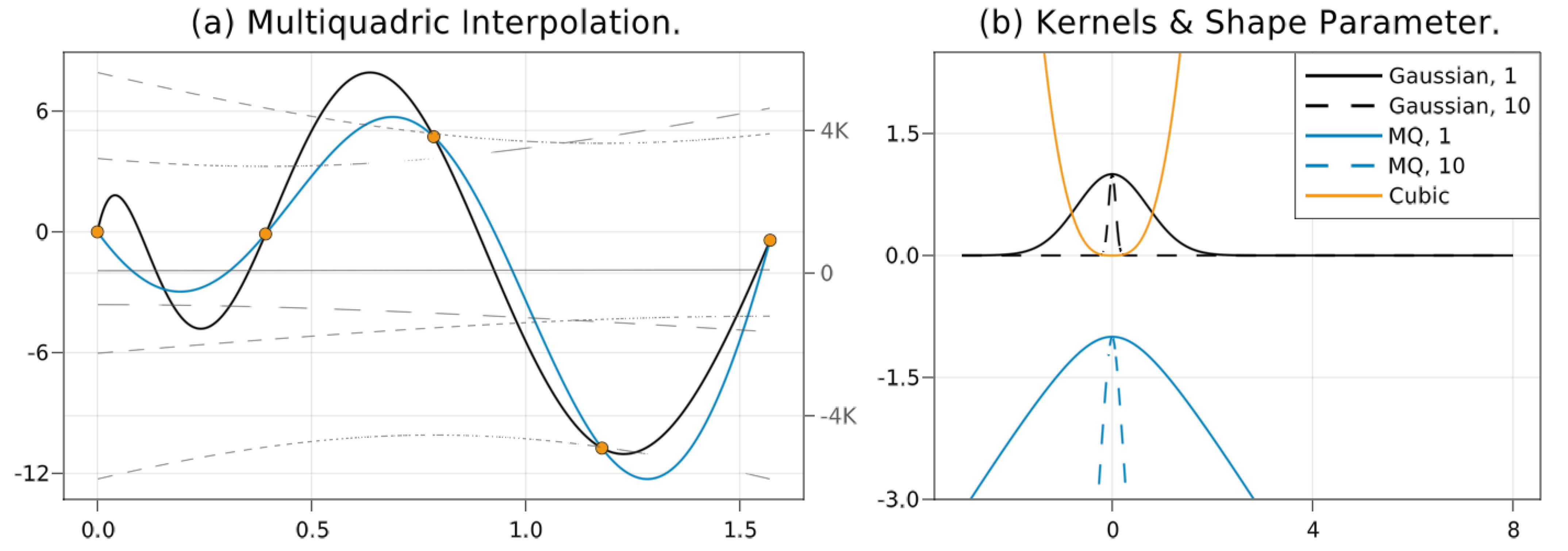
4.3. Fully Linear Radial Basis Function Models

The main drawback of quadratic Lagrange models is that we still need $\mathcal{O}\left(n^2\right)$ function evaluations in each iteration of Algorithm 2. A possible fix is to use under-determined regression polynomials instead [27,31,41]. Motivated by the findings in [34] we chose so-called Radial Basis Function (RBF) models as an alternative. RBF are well-known for their approximation capabilities on irregular data [40]. In our implementation they have the form

$$m\left(\mathbf{x}\right)=\sum _{i=1}^N{c}_i\phi \left({∥\mathbf{x}-{\xi }_i∥}_2\right)+\pi \left(\mathbf{x}\right),\mathrm{with}\pi =\sum _{j=1}^{n+1}{\lambda }_j{\psi }_j\in {\Pi }_n^1\mathrm{and}N\ge n+1,$$

(4)

which conforms to the construction by Wild et al. [34]. Here, $\phi$ is a function from a domain containing ${\mathbb{R}}_{\ge 0}$ to $\mathbb{R}$. For a fixed $\phi$ the mapping $\phi \left(∥•∥\right)$ from ${\mathbb{R}}^n\to \mathbb{R}$ is radially symmetric with respect to its argument and the mapping $(\mathbf{x},\xi )\mapsto \phi \left({∥\mathbf{x}-\xi ∥}_2\right)$ is called a kernel.

We will describe the procedure only briefly and refer to [34,42] and the dissertation [41] for more details. To conform to the algorithmic framework the models must have Hessians of uniformly bounded norm. Additionally, we want them to be twice differentiable due to the following, very general result:

Theorem 3

(Th 4.1 in [41]). Suppose that f and m are continuously differentiable in an open domain containing $B^{\left(t\right)}$ and that $\mathbf{\nabla }f$ and $\mathbf{\nabla }m$ are Lipschitz in $B^{\left(t\right)}$. Further suppose that m interpolates f on a Λ-poised set $\Xi =\{{\xi }_1,\dots ,{\xi }_{n+1}\}$ (for a fixed $\Lambda <\infty$). Then m is fully linear for f as in Definition 3.

The $\Lambda$-poised set is determined using pivotal algorithms from [34,41] in an enlarged trust region of radius ${\theta }_1{\Delta }^{\left(t\right)},{\theta }_1\ge 1$. If we restrict ourselves to functions $\phi$ that are conditionally positive definite (c.p.d.—see [34] for the definition) of order $D\le 2$, then for any $f:{\mathbb{R}}^n\to \mathbb{R}$ an interpolating model m of form (4) is uniquely determined by solving a linear equation system. If further $\phi$ is either twice continuously differentiable on an open domain containing $[0,\infty )$ with ${\phi }^{\prime }\left(0\right)=0,$ then m from (4) is twice continuously differentiable and has Lipschitz gradients exactly if its Hessian stays bounded. This is the case for all $\phi$ we consider (see

Table 1. Some radial functions $\phi :{\mathbb{R}}_{\ge 0}\to \mathbb{R}$ that are c.p.d. of order $D\le 2$, cf. [34].

Name	$\mathit{\phi }\left(\mathit{r}\right)$	c.p.d. order D
Cubic	$r^3$	2
Multiquadric	$-\sqrt{1+{\left(\alpha r\right)}^2},\alpha >0$	1
Gaussian	$exp(-{\left(\alpha r\right)}^2),\alpha >0$	0

). The hessian norm is determined by the magnitudes of the coefficients $c_i$ and by $|{\phi }^{\prime }\left(r\right)/r|$ and $|{\phi }^{″}\left(r\right)|$.

If there are exactly $N=n+1$ points from a poised set $\Xi$, then the coefficients $c_i$ vanish and the model (4) is a linear polynomial. The values $|{\phi }^{\prime }\left(r\right)/r|$ and $|{\phi }^{\prime \prime }\left(r\right)|$ are bounded because of $r\in [0,{\Delta }^{\mathrm{ub}}]$ and ${\phi }^{\prime }\left(0\right)=0$. To exploit the nonlinear modeling capabilities of RBF and perform exploration, there is a procedure in [34] to select additional (database) points from within a region of maximum radius ${\theta }_2{\Delta }^{\mathrm{ub}}$, ${\theta }_2\ge {\theta }_1\ge 1$, so that the values $|c_i|$ stay bounded. Modifications for box constraints can be found in [41] ([Sec. 6.3.1]) and [43].

Table 1 shows the RBF we are using and of which order they are. Both the Gaussian and the Multiquadric allow for fine-tuning with a shape parameter $\alpha >0$. This can potentially improve the conditioning of the interpolation system.

Figure 1b illustrates the effect of the shape parameter. As can be seen, the radial functions become narrower for larger shape parameters. Hence, we do not only use a constant shape parameter $\alpha =1$ like [34] do, but we also use an $\alpha$ that is (within lower and upper bounds) inversely proportional to ${\Delta }^{\left(t\right)}$.

Figure 1a shows interpolation of a nonlinear function by a surrogate based on the Multiquadric with a linear tail.

5. Descent Steps

In this section we introduce some possible steps ${\mathbf{s}}^{\left(t\right)}$ to use in Algorithm 2. We begin by defining the best step along the steepest descent direction as given by (Pm). Subsequently, backtracking variants are defined that use a multiobjective variant of Armijo’s rule.

5.1. Pareto–Cauchy Step

Both the Pareto–Cauchy point as well as a backtracking variant, the modified Pareto–Cauchy point, are points along the descent direction ${\mathbf{d}}_{\mathrm{m}}^{\left(t\right)}$ within $B^{\left(t\right)}$ so that a sufficient decrease measured by ${\Phi }_{\mathrm{m}}^{\left(t\right)}(•)$ and ${\omega }_{\mathrm{m}}^{\left(t\right)}\left(•\right)$ is achieved. Under mild assumptions we can then derive a decrease in terms of $\omega \left(•\right)$.

Definition 6.

For $t\in {\mathbb{N}}_0$ let ${\mathbf{d}}_{\mathrm{m}}^{\left(t\right)}$ be a minimizer for (Pm). The best attainable trial point ${\mathbf{x}}_{\mathrm{PC}}^{\left(t\right)}$ along ${\mathbf{d}}_{\mathrm{m}}^{\left(t\right)}$ is called the Pareto–Cauchy point and given by

$$\begin{array}{cc}\hfill {\mathbf{x}}_{\mathrm{PC}}^{\left(t\right)}& :={\mathbf{x}}^{\left(t\right)}+{\sigma }^{\left(t\right)}·{\mathbf{d}}_{\mathrm{m}}^{\left(t\right)},\hfill \\ \hfill & {\sigma }^{\left(t\right)}=\underset{0\le \sigma }{arg\; min}{\Phi }_{\mathrm{m}}^{\left(t\right)}\left({\mathbf{x}}^{\left(t\right)}+\sigma ·{\mathbf{d}}_{\mathrm{m}}^{\left(t\right)}\right)\hfill & \hfill \mathbf{s}.\mathbf{t}.{\mathbf{x}}_{\mathrm{PC}}^{\left(t\right)}\in B^{\left(t\right)}.\end{array}$$

(5)

Let ${\sigma }^{\left(t\right)}$ be the minimizer in (5). We call ${\mathbf{s}}_{\mathrm{PC}}^{\left(t\right)}:={\sigma }^{\left(t\right)}{\mathbf{d}}_{\mathrm{m}}^{\left(t\right)}$ the Pareto–Cauchy step.

If we make the following standard assumption, then the Pareto–Cauchy point allows for a lower bound on the improvement in terms of ${\Phi }_{\mathrm{m}}^{\left(t\right)}$.

Assumption 2.

For all $t\in {\mathbb{N}}_0$ the surrogates ${\mathrm{m}}^{\left(t\right)}\left(\mathbf{x}\right)={[m_1^{\left(t\right)}\left(\mathbf{x}\right),\dots ,m_k^{\left(t\right)}\left(\mathbf{x}\right)]}^T$ are twice continuously differentiable on an open set containing $\mathcal{X}$. Denote by $\mathit{H}{m}_{\ell }^{\left(t\right)}\left(\mathbf{x}\right)$ the Hessian of $m_{\ell }^{\left(t\right)}$ for $\ell =1,\dots ,k$.

Theorem 4.

If Assumptions 1 and 2 are satisfied, then for any iterate ${\mathbf{x}}^{\left(t\right)}$ the Pareto–Cauchy point ${\mathbf{x}}_{\mathrm{PC}}^{\left(t\right)}$ satisfies

$${\Phi }_{\mathrm{m}}^{\left(t\right)}\left({\mathbf{x}}^{\left(t\right)}\right)-{\Phi }_{\mathrm{m}}^{\left(t\right)}\left({\mathbf{x}}_{\mathrm{PC}}^{\left(t\right)}\right)\ge \frac{1}{2}{\omega }_{\mathrm{m}}^{\left(t\right)}\left({\mathbf{x}}^{\left(t\right)}\right)·min\left\{\frac{{\omega }_{\mathrm{m}}^{\left(t\right)}\left({\mathbf{x}}^{\left(t\right)}\right)}{\mathrm{c}{H}_{\mathrm{m}}^{\left(t\right)}},{\Delta }^{\left(t\right)},1\right\},$$

(6)

where

$$H_{\mathrm{m}}^{\left(t\right)}=\underset{\ell =1,\dots ,k}{max}\underset{\mathbf{x}\in B^{\left(t\right)}}{max}{∥\mathit{H}{m}_{\ell }^{\left(t\right)}\left(\mathbf{x}\right)∥}_F$$

(7)

and the constant $\mathrm{c}>0$ relates the trust region norm $∥•∥$ to the Euclidean norm ${∥•∥}_2$ via

$${∥\mathbf{x}∥}_2\le \sqrt{\mathrm{c}}∥\mathbf{x}∥\forall \mathbf{x}\in {\mathbb{R}}^n.$$

(8)

If $∥•∥={∥•∥}_{\infty }$ is used, then $\mathrm{c}$ can be chosen as $\mathrm{c}=k$. The proof for Theorem 4 is provided after the next auxiliary lemma.

Lemma 2.

Under Assumptions 1 and 2, let $\mathbf{d}$ be a non-increasing direction at ${\mathbf{x}}^{\left(t\right)}\in {\mathbb{R}}^n$ for ${\mathrm{m}}^{\left(t\right)}$, i.e.,

$$〈\mathbf{\nabla }{m}_{\ell }^{\left(t\right)}\left({\mathbf{x}}^{\left(t\right)}\right),\mathbf{d}〉\le 0\forall \ell =1,\dots ,k.$$

Let $q\in \{1,\dots ,k\}$ be any objective index and $\overline{\sigma }\ge min\left\{{\Delta }^{\left(t\right)},∥\mathbf{d}∥\right\}$. Then it holds that

$$m_q^{\left(t\right)}\left({\mathbf{x}}^{\left(t\right)}\right)-\underset{0<\sigma <\overline{\sigma }}{min}{m}_q^{\left(t\right)}\left({\mathbf{x}}^{\left(t\right)}+\sigma \frac{\mathbf{d}}{∥\mathbf{d}∥}\right)\ge \frac{w}{2}min\left\{\frac{w}{{∥\mathbf{d}∥}^2\mathrm{c}{H}_{\mathrm{m}}^{\left(t\right)}},\frac{{\Delta }^{\left(t\right)}}{∥\mathbf{d}∥},1\right\},$$

where we have used the shorthand notation

$$w=-\underset{\ell =1,\dots ,k}{max}〈\mathbf{\nabla }{m}_{\ell }^{\left(t\right)}\left({\mathbf{x}}^{\left(t\right)}\right),\mathbf{d}〉\ge 0.$$

Lemma 2 states that a minimizer along any non-increasing direction $\mathbf{d}$ achieves a minimum reduction w.r.t. ${\Phi }_{\mathrm{m}}^{\left(t\right)}$. Similar results can be found in in [30] or [33]. But since we do not use polynomial surrogates ${\mathrm{m}}^{\left(t\right)}$, we have to employ the multivariate version of Taylor’s theorem to make the proof work. We can do this because according to Assumption 2, the  functions $m_q^{\left(t\right)},q\in \{1,\dots ,k\}$ are twice continuously differentiable in an open domain containing $\mathcal{X}$. Moreover, Assumption 1 ensures that the function is defined on the line from χ to $\mathbf{x}$. As shown in [44] (Ch. 3) a first degree expansion at $\mathbf{x}\in B(\chi ,\Delta )$ around $\chi \in \mathcal{X}$ then leads to

$$\begin{array}{ccc}\hfill & m_q^{\left(t\right)}\left(\mathbf{x}\right)=m_q(\chi )+\mathbf{\nabla }{m}_q^{\left(t\right)}{(\chi )}^T\mathbf{h}+\frac{1}{2}{\mathbf{h}}^T\mathit{H}{m}_q^{\left(t\right)}\left({\xi }_q\right)\mathbf{h},\hfill & \hfill \mathrm{with}\mathbf{h}=\left(\mathbf{x}-\chi \right),\\ \hfill & \mathrm{for}\mathrm{some}{\xi }_q\in \left\{\mathbf{x}+\theta \left(\chi -\mathbf{x}\right):\theta \in [0,1]\right\},\mathrm{for}\mathrm{all}q=1,\dots ,k.\hfill \end{array}$$

(9)

Proof of Lemma 2. 

Let the requirements of Lemma 2 hold and let $\mathbf{d}$ be a non-increasing direction for ${\mathbf{m}}^{\left(t\right)}$. Then:

$$\begin{array}{cc}\hfill & m_q^{\left(t\right)}\left({\mathbf{x}}^{\left(t\right)}\right)-\underset{0<\sigma <\overline{\sigma }}{min}{m}_q^{\left(t\right)}\left({\mathbf{x}}^{\left(t\right)}+\sigma \frac{\mathbf{d}}{∥\mathbf{d}∥}\right)=\underset{0\le \sigma \le \overline{\sigma }}{max}\left\{m_q^{\left(t\right)}\left({\mathbf{x}}^{\left(t\right)}\right)-m_q^{\left(t\right)}\left({\mathbf{x}}^{\left(t\right)}+\sigma \frac{\mathbf{d}}{∥\mathbf{d}∥}\right)\right\}\hfill \\ \hfill & \stackrel{\left(9\right)}{=}\underset{0\le \sigma \le \overline{\sigma }}{max}\left\{m_q^{\left(t\right)}\left({\mathbf{x}}^{\left(t\right)}\right)-\left(m_q^{\left(t\right)}\left({\mathbf{x}}^{\left(t\right)}\right)+\frac{\sigma }{∥\mathbf{d}∥}\langle \mathbf{\nabla }{m}_q^{\left(t\right)}\left({\mathbf{x}}^{\left(t\right)}\right),\mathbf{d}\rangle +\frac{{\sigma }^2}{2{∥\mathbf{d}∥}^2}\langle \mathbf{d},\mathit{H}{m}_q^{\left(t\right)}\left({\xi }_q\right)\mathbf{d}\rangle \right)\right\}\hfill \\ \hfill & \ge \underset{0\le \sigma \le \overline{\sigma }}{max}\left\{-\frac{\sigma }{∥\mathbf{d}∥}\underset{j=1,\dots ,k}{max}\langle \mathbf{\nabla }{m}_j^{\left(t\right)}\left({\mathbf{x}}^{\left(t\right)}\right),\mathbf{d}\rangle -\frac{{\sigma }^2}{2{∥\mathbf{d}∥}^2}\langle \mathbf{d},\mathit{H}{m}_q^{\left(t\right)}\left({\xi }_q\right)\mathbf{d}\rangle \right\}.\hfill \end{array}$$

We used the shorthand $w=-\underset{j}{max}\langle \mathbf{\nabla }{m}_j^{\left(t\right)}\left({\mathbf{x}}^{\left(t\right)}\right),\mathbf{d}\rangle$ and the Cauchy-Schwartz inequality to get

$$\begin{array}{c}\hfill \cdots \ge \underset{0\le \sigma \le \overline{\sigma }}{max}\left\{\frac{\sigma }{∥\mathbf{d}∥}w-\frac{{\sigma }^2}{2{∥\mathbf{d}∥}^2}{∥\mathbf{d}∥}_2^2{∥\mathit{H}{m}_q^{\left(t\right)}(\xi )∥}_F\right\}\stackrel{\left(8\right),\left(7\right)}{\ge }\underset{0\le \sigma \le \overline{\sigma }}{max}\left\{\frac{\sigma }{∥\mathbf{d}∥}w-\frac{{\sigma }^2}{2}\mathrm{c}{H}_{\mathrm{m}}^{\left(t\right)}\right\}.\end{array}$$

The RHS is concave and we can thus easily determine the global maximizer ${\sigma }^{*}$.

Similar to [30] (Lemma 4.1) we find

$$\begin{array}{cc}\hfill m_q^{\left(t\right)}\left({\mathbf{x}}^{\left(t\right)}\right)-\underset{0<\sigma <\overline{\sigma }}{min}{m}_q^{\left(t\right)}\left({\mathbf{x}}^{\left(t\right)}+\sigma \frac{\mathbf{d}}{∥\mathbf{d}∥}\right)& \ge \frac{w}{2}min\left\{\frac{w}{{∥\mathbf{d}∥}^2\mathrm{c}{H}_{\mathrm{m}}^{\left(t\right)}},\frac{{\Delta }^{\left(t\right)}}{∥\mathbf{d}∥},1\right\},\hfill \end{array}$$

where we have additionally used $\overline{\sigma }\ge min\{{\Delta }^{\left(t\right)},1\}$.    □

Proof of Theorem 4. 

If ${\mathbf{x}}^{\left(t\right)}$ is Pareto critical for (MOPm), then ${\mathbf{d}}_{\mathrm{m}}^{\left(t\right)}=0$ and ${\omega }_{\mathrm{m}}^{\left(t\right)}\left({\mathbf{x}}^{\left(t\right)}\right)=0$ and the inequality holds trivially.

Else, let the indices $\ell ,q\in \{1,\dots ,k\}$ be such that

$${\Phi }_{\mathrm{m}}^{\left(t\right)}\left({\mathbf{x}}^{\left(t\right)}\right)-{\Phi }_{\mathrm{m}}^{\left(t\right)}\left({\mathbf{x}}_{\mathrm{PC}}^{\left(t\right)}\right)=m_{\ell }^{\left(t\right)}\left({\mathbf{x}}^{\left(t\right)}\right)-m_q^{\left(t\right)}\left({\mathbf{x}}_{\mathrm{PC}}^{\left(t\right)}\right)\ge m_q\left({\mathbf{x}}^{\left(t\right)}\right)-m_q\left({\mathbf{x}}_{\mathrm{PC}}^{\left(t\right)}\right)$$

and define

$$\overline{\sigma }:=\left\{\begin{array}{cc}min\left\{{\Delta }^{\left(t\right)},∥{\mathbf{d}}_{\mathrm{m}}^{\left(t\right)}∥\right\}\hfill & \mathrm{if}∥{\mathbf{d}}_{\mathrm{m}}^{\left(t\right)}∥<1\mathrm{or}{\Delta }^{\left(t\right)}\le 1,\hfill \\ {\Delta }^{\left(t\right)}\hfill & \mathrm{else}.\hfill \end{array}\right.$$

(10)

Then clearly $\overline{\sigma }\ge min\left\{{\Delta }^{\left(t\right)},∥{\mathbf{d}}_{\mathrm{m}}^{\left(t\right)}∥\right\}$ and for the Pareto–Cauchy point we have

$$m_q^{\left(t\right)}\left({\mathbf{x}}_{\mathrm{PC}}^{\left(t\right)}\right)=\underset{0\le \sigma \le \overline{\sigma }}{min}{m}_q\left({\mathbf{x}}^{\left(t\right)}+\frac{\sigma }{∥{\mathbf{d}}_{\mathrm{m}}^{\left(t\right)}∥}{\mathbf{d}}_{\mathrm{m}}^{\left(t\right)}\right).$$

From Lemma 2 and $∥{\mathbf{d}}_{\mathrm{m}}^{\left(t\right)}∥$ the bound $\left(6\right)$ immediately follows.    □

Remark 4.

Some authors define the Pareto–Cauchy point as the actual minimizer ${\mathbf{x}}_{min}^{\left(t\right)}$ of ${\Phi }_{\mathrm{m}}^{\left(t\right)}$ within the current trust region (instead of the minimizer along the steepest descent direction). For this true minimizer the same bound (6) holds. This is due to

$$\begin{array}{c}\hfill {\Phi }_{\mathrm{m}}^{\left(t\right)}\left({\mathbf{x}}^{\left(t\right)}\right)-{\Phi }_{\mathrm{m}}^{\left(t\right)}\left({\mathbf{x}}_{min}^{\left(t\right)}\right)=m_{\ell }\left({\mathbf{x}}^{\left(t\right)}\right)-\underset{\mathbf{x}\in B^{\left(t\right)}}{min}{m}_q\left(\mathbf{x}\right)\ge m_q\left({\mathbf{x}}^{\left(t\right)}\right)-m_q\left({\mathbf{x}}_{\mathrm{PC}}^{\left(t\right)}\right).\end{array}$$

5.2. Modified Pareto–Cauchy Point via Backtracking

A common approach in trust region methods is to find an approximate solution to (5) within the current trust region. Usually a backtracking procedure similar to Armijo’s inexact line-search is used for the Pareto–Cauchy subproblem, see [36] (Section 6.3) and [30]. Doing so, we can still guarantee a sufficient decrease.

Before we actually define the backtracking step along ${\mathbf{d}}_{\mathrm{m}}^{\left(t\right)}$, we derive a more general lemma. It illustrates that backtracking along any suitable direction is well-defined.

Lemma 3.

Suppose Assumptions 1 and 2 hold. For ${\mathbf{x}}^{\left(t\right)}\in {\mathbb{R}}^n$, let $\mathbf{d}$ be a descent direction for ${\mathrm{m}}^{\left(t\right)}$ and let $q\in \{1,\dots ,k\}$ be any objective index and $\overline{\sigma }>0$. Then, for any fixed constants $\mathrm{a},\mathrm{b}\in (0,1)$ there is an integer $j\in {\mathbb{N}}_0$ such that

$$\Psi \left({\mathbf{x}}^{\left(t\right)}+\frac{{\mathrm{b}}^j\overline{\sigma }}{∥\mathbf{d}∥}\mathbf{d}\right)\le \Psi \left({\mathbf{x}}^{\left(t\right)}\right)-\frac{\mathrm{a}{\mathrm{b}}^j\overline{\sigma }}{∥\mathbf{d}∥}w$$

(11)

where, again, we have used the shorthand notation $w=-{max}_{\ell =1,\dots ,k}〈\mathbf{\nabla }{m}_{\ell }^{\left(t\right)}\left({\mathbf{x}}^{\left(t\right)}\right),\mathbf{d}〉>0$ and Ψ is either some specific model, $\Psi =m_{\ell }$, or the maximum value, $\Psi ={\Phi }_{\mathrm{m}}^{\left(t\right)}$.

Moreover, if we define the step ${\mathbf{s}}^{\left(t\right)}=\frac{{\mathrm{b}}^j\overline{\sigma }}{∥\mathbf{d}∥}\mathbf{d}$ for thesmallest$j\in {\mathbb{N}}_0$ satisfying (11), then there is a constant ${\kappa }_{\mathrm{m}}^{\mathrm{sd}}\in (0,1)$ such that

$$\Psi \left({\mathbf{x}}^{\left(t\right)}\right)-\Psi \left({\mathbf{x}}^{\left(t\right)}+{\mathbf{s}}^{\left(t\right)}\right)\ge {\kappa }_{\mathrm{m}}^{\mathrm{sd}}wmin\left\{\frac{w}{{∥\mathbf{d}∥}^2\mathrm{c}{H}_{\mathrm{m}}^{\left(t\right)}},\frac{\overline{\sigma }}{∥\mathbf{d}∥}\right\}.$$

(12)

Proof. 

The first part can be derived from the fact that $\mathbf{d}$ is a descent direction, see e.g., [6]. However, we will use the approach from [30] to also derive the bound (12). With Taylor’s Theorem we obtain

$$\begin{array}{cc}\hfill & \Psi \left({\mathbf{x}}^{\left(t\right)}+\frac{{\mathrm{b}}^j\overline{\sigma }}{∥\mathbf{d}∥}\mathbf{d}\right)=m_{\ell }\left({\mathbf{x}}^{\left(t\right)}+\frac{{\mathrm{b}}^j\overline{\sigma }}{∥\mathbf{d}∥}\mathbf{d}\right)(\mathrm{for}\mathrm{some}\ell \in \{1,\dots ,k\})\hfill \\ & =m_{\ell }^{\left(t\right)}\left({\mathbf{x}}^{\left(t\right)}\right)+\frac{{\mathrm{b}}^j\overline{\sigma }}{∥\mathbf{d}∥}\langle \mathbf{\nabla }{m}_{\ell }^{\left(t\right)}\left({\mathbf{x}}^{\left(t\right)}\right),\mathbf{d}\rangle +\frac{{\left({\mathrm{b}}^j\overline{\sigma }\right)}^2}{2{∥\mathbf{d}∥}^2}\langle \mathbf{d},\mathit{H}{m}_{\ell }^{\left(t\right)}\left({\xi }_{\ell }\right)\mathbf{d}\rangle \hfill \\ & \le \Psi \left({\mathbf{x}}^{\left(t\right)}\right)+\underset{q=1,\dots ,k}{max}\frac{{\mathrm{b}}^j\overline{\sigma }}{∥\mathbf{d}∥}\langle \mathbf{\nabla }{m}_q^{\left(t\right)}\left({\mathbf{x}}^{\left(t\right)}\right),\mathbf{d}\rangle +\underset{q=1,\dots ,k}{max}\frac{{\left({\mathrm{b}}^j\overline{\sigma }\right)}^2}{2{∥\mathbf{d}∥}^2}\langle \mathbf{d},\mathit{H}{m}_q^{\left(t\right)}\left({\xi }_q\right)\mathbf{d}\rangle \hfill \end{array}$$

$$\begin{array}{c}\hfill \stackrel{\left(\mathrm{Pm}\right),\left(7\right)}{\le }\Psi \left({\mathbf{x}}^{\left(t\right)}\right)-\frac{{\mathrm{b}}^j\overline{\sigma }}{∥\mathbf{d}∥}w+\frac{{\left({\mathrm{b}}^j\overline{\sigma }\right)}^2}{2}\mathrm{c}{H}_{\mathrm{m}}^{\left(t\right)}.\end{array}$$

(13)

In the last line, we have additionally used the Cauchy–Schwartz inequality. For a constructive proof, suppose now that (11) is violated for some $j\in {\mathbb{N}}_0$, i.e.,

$$\Psi \left({\mathbf{x}}^{\left(t\right)}+\frac{{\mathrm{b}}^j\overline{\sigma }}{∥\mathbf{d}∥}\mathbf{d}\right)>\Psi \left({\mathbf{x}}^{\left(t\right)}\right)-\frac{\mathrm{a}{\mathrm{b}}^j\overline{\sigma }}{∥\mathbf{d}∥}w.$$

Plugging in (13) for the LHS and substracting $\Psi \left({\mathbf{x}}^{\left(t\right)}\right)$ then leads to

$${\mathrm{b}}^j>\frac{2(1-\mathrm{a})w}{∥\mathbf{d}∥\overline{\sigma }\mathrm{c}{H}_{\mathrm{m}}^{\left(t\right)}},$$

where the right hand side is positive and completely independent of j. Since $\mathrm{b}\in (0,1)$, there must be a $j^{*}\in {\mathbb{N}}_0,j^{*}>j,$ for which ${\mathrm{b}}^{j^{*}}\le {\displaystyle \frac{2(1-\mathrm{a})w}{∥\mathbf{d}∥\overline{\sigma }\mathrm{c}{H}_{\mathrm{m}}^{\left(t\right)}}}$ so that (11) must also be fulfilled for this ${\mathrm{b}}^{j^{*}}$.

Analogous to the proof of [30] ([Lemma 4.2]) we can now derive the constant ${\kappa }_{\mathrm{m}}^{\mathrm{sd}}$ from (12) as ${\kappa }_{\mathrm{m}}^{\mathrm{sd}}=min\{2\mathrm{b}(1-\mathrm{a}),\mathrm{a}\}.$

   □

Lemma 3 applies naturally to the step along ${\mathbf{d}}_{\mathrm{m}}^{\left(t\right)}$:

Definition 7.

For ${\mathbf{x}}^{\left(t\right)}\in B^{\left(t\right)}$ let ${\mathbf{d}}_{\mathrm{m}}^{\left(t\right)}$ be a solution to $\left(\mathrm{Pm}\right)$ and define the modified Pareto–Cauchy step as

$${\tilde{\mathbf{s}}}_{\mathrm{PC}}^{\left(t\right)}:={\mathrm{b}}^j\overline{\sigma }\frac{{\mathbf{d}}_{\mathrm{m}}^{\left(t\right)}}{∥{\mathbf{d}}_{\mathrm{m}}^{\left(t\right)}∥},$$

where again $\overline{\sigma }$ as in (10) and $j\in {\mathbb{N}}_0$ is the smallest integer that satisfies

$${\Phi }_{\mathrm{m}}^{\left(t\right)}({\mathbf{x}}^{\left(t\right)}+{\tilde{\mathbf{s}}}_{\mathrm{PC}}^{\left(t\right)})\le {\Phi }_{\mathrm{m}}^{\left(t\right)}\left({\mathbf{x}}^{\left(t\right)}\right)-\frac{\mathrm{a}{\mathrm{b}}^j\overline{\sigma }}{∥{\mathbf{d}}_{\mathrm{m}}^{\left(t\right)}∥}{\omega }_{\mathrm{m}}^{\left(t\right)}\left({\mathbf{x}}^{\left(t\right)}\right)$$

(14)

for predefined constants $\mathrm{a},\mathrm{b}\in (0,1)$.

The definition of $\overline{\sigma }$ ensures, that ${\mathbf{x}}^{\left(t\right)}+{\tilde{\mathbf{s}}}_{\mathrm{PC}}^{\left(t\right)}$ is contained in the current trust region $B^{\left(t\right)}$. Furthermore, these steps provide a sufficient decrease very similar to (6):

Corollary 1.

Suppose Assumptions 1 and 2 hold. For the step ${\tilde{\mathbf{s}}}_{\mathrm{PC}}^{\left(t\right)}$ the following statements are true:

• A $j\in {\mathbb{N}}_0$ as in (14) exists.
• There is a constant ${\kappa }_{\mathrm{m}}^{\mathrm{sd}}\in (0,1)$ such that the modified Pareto–Cauchy step ${\tilde{\mathbf{s}}}_{\mathrm{PC}}^{\left(t\right)}$ satisfies

  $${\Phi }_{\mathrm{m}}^{\left(t\right)}\left({\mathbf{x}}^{\left(t\right)}\right)-{\Phi }_{\mathrm{m}}^{\left(t\right)}({\mathbf{x}}^{\left(t\right)}+{\tilde{\mathbf{s}}}_{\mathrm{PC}}^{\left(t\right)})\ge {\kappa }_{\mathrm{m}}^{\mathrm{sd}}{\omega }_{\mathrm{m}}^{\left(t\right)}\left({\mathbf{x}}^{\left(t\right)}\right)min\left\{\frac{{\omega }_{\mathrm{m}}^{\left(t\right)}\left({\mathbf{x}}^{\left(t\right)}\right)}{\mathrm{c}{H}_{\mathrm{m}}^{\left(t\right)}},{\Delta }^{\left(t\right)},1\right\}.$$

Proof. 

If ${\mathbf{x}}^{\left(t\right)}$ is critical, then the bound is trivial. Otherwise, the existence of a j satisfying (14) follows from Lemma 3 for $\Psi ={\Phi }_{\mathrm{m}}^{\left(t\right)}$. The lower bound on the decrease follows immediately from $\overline{\sigma }\ge min\left\{∥{\mathbf{d}}_{\mathrm{m}}^{\left(t\right)}∥,{\Delta }^{\left(t\right)}\right\}$.    □

From Lemma 3 it follows that the backtracking condition (14) can be modified to explicitly require a decrease in every objective:

Definition 8.

Let $j\in {\mathbb{N}}_0$ the smallest integer satisfying

$$\underset{\ell =1,\dots ,k}{min}\left\{m_{\ell }^{\left(t\right)}\left({\mathbf{x}}^{\left(t\right)}\right)-m_{\ell }^{\left(t\right)}\left({\mathbf{x}}^{\left(t\right)}+{\mathrm{b}}^j\overline{\sigma }\frac{{\mathbf{d}}_{\mathrm{m}}^{\left(t\right)}}{∥{\mathbf{d}}_{\mathrm{m}}^{\left(t\right)}∥}\right)\right\}\ge \frac{\mathrm{a}{\mathrm{b}}^j\overline{\sigma }}{∥{\mathbf{d}}_{\mathrm{m}}^{\left(t\right)}∥}{\omega }_{\mathrm{m}}^{\left(t\right)}\left({\mathbf{x}}^{\left(t\right)}\right).$$

We define the strict modified Pareto–Cauchy point as ${\widehat{\mathbf{x}}}_{\mathrm{PC}}^{\left(t\right)}={\mathbf{x}}^{\left(t\right)}+{\widehat{\mathbf{s}}}_{\mathrm{PC}}^{\left(t\right)}$ and the corresponding step as ${\widehat{\mathbf{s}}}_{\mathrm{PC}}^{\left(t\right)}={\mathrm{b}}^j\overline{\sigma }{\displaystyle \frac{{\mathbf{d}}_{\mathrm{m}}^{\left(t\right)}}{∥{\mathbf{d}}_{\mathrm{m}}^{\left(t\right)}∥}}$.

Corollary 2.

Suppose Assumptions 1 and 2 hold.

1

The strict modified Pareto–Cauchy point exists, the backtracking is finite.

2

There is a constant ${\kappa }_{\mathrm{m}}^{\mathrm{sd}}\in (0,1)$ such that

$$\underset{\ell =1,\dots ,k}{min}\left\{m_{\ell }^{\left(t\right)}\left({\mathbf{x}}^{\left(t\right)}\right)-m_{\ell }^{\left(t\right)}\left({\widehat{\mathbf{x}}}_{\mathrm{PC}}^{\left(t\right)}\right)\right\}\ge {\kappa }_{\mathrm{m}}^{\mathrm{sd}}{\omega }_{\mathrm{m}}^{\left(t\right)}\left({\mathbf{x}}^{\left(t\right)}\right)min\left\{\frac{{\omega }_{\mathrm{m}}^{\left(t\right)}\left({\mathbf{x}}^{\left(t\right)}\right)}{\mathrm{c}{H}_{\mathrm{m}}^{\left(t\right)}},{\Delta }^{\left(t\right)},1\right\}.$$

(15)

Remark 5.

In the preceding subsections, we have shown descent steps along the model steepest descent direction. Similar to the single objective case we do not necessarily have to use the steepest descent direction and different step calculation methods are viable. For instance, Thomann and Eichfelder [33] use the well-known Pascoletti–Serafini scalarization to treat the subproblem (MOPm). We refer to their work and Appendix B to see how this method can be related to the steepest descent direction.

5.3. Sufficient Decrease for the Original Problem

In the previous subsections, we have shown how to compute steps ${\mathbf{s}}^{\left(t\right)}$ to achieve a sufficient decrease in terms of ${\Phi }_{\mathrm{m}}^{\left(t\right)}$ and ${\omega }_{\mathrm{m}}^{\left(t\right)}\left(•\right)$. For a descent step ${\mathbf{s}}^{\left(t\right)}$ the bound is of the form

$${\Phi }_{\mathrm{m}}^{\left(t\right)}\left({\mathbf{x}}^{\left(t\right)}\right)-{\Phi }_{\mathrm{m}}^{\left(t\right)}({\mathbf{x}}^{\left(t\right)}+{\mathbf{s}}^{\left(t\right)})\ge {\kappa }_{\mathrm{m}}^{\mathrm{sd}}{\omega }_{\mathrm{m}}^{\left(t\right)}\left({\mathbf{x}}^{\left(t\right)}\right)min\left\{\frac{{\omega }_{\mathrm{m}}^{\left(t\right)}\left({\mathbf{x}}^{\left(t\right)}\right)}{\mathrm{c}{H}_{\mathrm{m}}^{\left(t\right)}},{\Delta }^{\left(t\right)},1\right\},{\kappa }_{\mathrm{m}}^{\mathrm{sd}}\in (0,1),$$

(16)

and thereby very similar to the bounds for the scalar projected gradient trust region method [36]. By introducing a slightly modified version of ${\omega }_{\mathrm{m}}^{\left(t\right)}\left(•\right)$, we can transform (16) into the bound used in [30,33].

Lemma 4.

If $\pi (t,{\mathbf{x}}^{\left(t\right)})$ is a criticality measure for some multiobjective problem, then $\tilde{\pi }(t,{\mathbf{x}}^{\left(t\right)})=min\left\{1,\pi (t,{\mathbf{x}}^{\left(t\right)})\right\}$ is also a criticality measure for the same problem.

Proof. 

We have $0\le \tilde{\pi }(t,{\mathbf{x}}^{\left(t\right)})\le \pi (t,{\mathbf{x}}^{\left(t\right)})$. Thus, $\tilde{\pi }\to 0$ whenever $\pi \to 0$. The minimum of uniformly continuous functions is again uniformly continuous.    □

We next make another standard assumption on the class of surrogate models.

Assumption 3.

The norm of all model hessians is uniformly bounded above on $\mathcal{X}$, i.e., there is a positive constant ${\mathrm{H}}_{\mathrm{m}}$ such that

$${∥\mathit{H}{m}_{\ell }^{\left(t\right)}\left(\mathbf{x}\right)∥}_F\le {\mathrm{H}}_{\mathrm{m}}\forall \ell =1,\dots ,k,\forall \mathbf{x}\in B^{\left(t\right)},\forall t\in {\mathbb{N}}_0.$$

W.l.o.g., we assume

$${\mathrm{H}}_{\mathrm{m}}·\mathrm{c}>1,with\mathrm{c}asin\left(8\right).$$

(17)

Remark 6.

From this assumption it follows that the model gradients are then Lipschitz as well. Together with Theorem 2, we then know that ${\omega }_{\mathrm{m}}^{\left(t\right)}\left(•\right)$ is a criticality measure for (MOPm).

Motivated by the previous remark, we will from now on refer to the following functions

$$\begin{array}{cc}\hfill \varpi \left(\mathbf{x}\right):=min\left\{\omega \left(\mathbf{x}\right),1\right\}\mathrm{and}{\varpi }_{\mathrm{m}}^{\left(t\right)}\left(\mathbf{x}\right):=min\left\{{\omega }_{\mathrm{m}}^{\left(t\right)}\left(\mathbf{x}\right),1\right\}& \forall t=0,1,\dots \hfill \end{array}$$

(18)

We can thereby derive the sufficient decrease condition in “standard form”:

Corollary 3.

Under Assumption 3, suppose that for ${\mathbf{x}}^{\left(t\right)}$ and some descent step ${\mathbf{s}}^{\left(t\right)}$ the bound (16) holds. For the criticality measure ${\varpi }_{\mathrm{m}}^{\left(t\right)}\left(•\right)$ it follows that

$${\Phi }_{\mathrm{m}}^{\left(t\right)}\left({\mathbf{x}}^{\left(t\right)}\right)-{\Phi }_{\mathrm{m}}^{\left(t\right)}({\mathbf{x}}^{\left(t\right)}+{\mathbf{s}}^{\left(t\right)})\ge {\kappa }_{\mathrm{m}}^{\mathrm{sd}}{\varpi }_{\mathrm{m}}^{\left(t\right)}\left({\mathbf{x}}^{\left(t\right)}\right)min\left\{\frac{{\varpi }_{\mathrm{m}}^{\left(t\right)}\left({\mathbf{x}}^{\left(t\right)}\right)}{\mathrm{c}{\mathrm{H}}_{\mathrm{m}}},{\Delta }^{\left(t\right)}\right\}.$$

(19)

Proof. 

${\varpi }_{\mathrm{m}}^{\left(t\right)}\left(•\right)$ is a criticality measure due to Assumption 3 and Lemma 4. Further, from (18) and (17) it follows that

$$\frac{{\varpi }_{\mathrm{m}}^{\left(t\right)}\left({\mathbf{x}}^{\left(t\right)}\right)}{\mathrm{c}{\mathrm{H}}_{\mathrm{m}}}\le \frac{1}{\mathrm{c}{\mathrm{H}}_{\mathrm{m}}}\le 1$$

and if we plug this into (16) we obtain (19).    □

To relate the RHS of (19) to the criticality $\omega \left(•\right)$ of the original problem, we require another assumption.

Assumption 4.

There is a constant ${\kappa }_{\omega }>0$ such that

$$\left|{\omega }_{\mathrm{m}}^{\left(t\right)}\left({\mathbf{x}}^{\left(t\right)}\right)-\omega \left({\mathbf{x}}^{\left(t\right)}\right)\right|\le {\kappa }_{\omega }{\omega }_{\mathrm{m}}^{\left(t\right)}\left({\mathbf{x}}^{\left(t\right)}\right).$$

This assumption is also made by Thomann and Eichfelder [33] and can easily be justified by using fully linear surrogate models and a bounded trust region radius in combination with a criticality test, see Lemma 7.

Assumption 4 can be used to formulate the next two lemmata relating the model criticality and the true criticality. They are proven in Appendix A.2. From these lemmata and Corollary 3 the final result, Corollary 4, easily follows.

Lemma 5.

If Assumption 4 holds, then it holds for ${\varpi }_{\mathrm{m}}^{\left(t\right)}\left(•\right)$ and $\varpi \left(•\right)$ from (18) that

$$\left|{\varpi }_{\mathrm{m}}^{\left(t\right)}\left({\mathbf{x}}^{\left(t\right)}\right)-\varpi \left({\mathbf{x}}^{\left(t\right)}\right)\right|\le {\kappa }_{\omega }{\varpi }_{\mathrm{m}}^{\left(t\right)}\left({\mathbf{x}}^{\left(t\right)}\right).$$

Lemma 6.

From Assumption 4 it follows that

$${\varpi }_{\mathrm{m}}^{\left(t\right)}\left({\mathbf{x}}^{\left(t\right)}\right)\ge \frac{1}{{\kappa }_{\omega }+1}\varpi \left({\mathbf{x}}^{\left(t\right)}\right)\mathrm{with}{({\kappa }_{\omega }+1)}^{-1}\in (0,1).$$

Corollary 4.

Suppose that Assumptions 3 and 4 hold and that ${\mathbf{x}}^{\left(t\right)}$ and ${\mathbf{s}}^{\left(t\right)}$ satisfy (19). Then

$$\begin{array}{cc}\hfill {\Phi }_{\mathrm{m}}^{\left(t\right)}\left({\mathbf{x}}^{\left(t\right)}\right)-{\Phi }_{\mathrm{m}}^{\left(t\right)}({\mathbf{x}}^{\left(t\right)}+{\mathbf{s}}^{\left(t\right)})& \ge {\kappa }^{\mathrm{sd}}\varpi \left({\mathbf{x}}^{\left(t\right)}\right)min\left\{\frac{\varpi \left({\mathbf{x}}^{\left(t\right)}\right)}{\mathrm{c}{\mathrm{H}}_{\mathrm{m}}},{\Delta }^{\left(t\right)}\right\},\hfill \end{array}$$

(20)

where ${\kappa }^{\mathrm{sd}}=\frac{{\kappa }_{\mathrm{m}}^{\mathrm{sd}}}{1+{\kappa }_{\omega }}\in (0,1)$.

6. Convergence

6.1. Preliminary Assumptions and Definitions

To prove convergence of Algorithm 2 we first have to make sure that at least one of the objectives is bounded from below. This is a weaker requirement than the standard assumption that all objectives are bounded from below:

Assumption 5.

The maximum ${max}_{\ell =1,\dots ,k}{f}_{\ell }\left(\mathbf{x}\right)$ of all objective functions is bounded from below on $\mathcal{X}$.

To be able to use $\varpi \left(•\right)$ as a criticality measure and to refer to fully linear models, we further require:

Assumption 6.

The objective $\mathbf{f}:{\mathbb{R}}^n\to {\mathbb{R}}^k$ is continuously differentiable in an open domain containing $\mathcal{X}$ and has a Lipschitz continuous gradient on $\mathcal{X}$.

We summarize the assumptions on the surrogates as follows:

Assumption 7.

The vector of surrogate model functions $m_1^{\left(t\right)},\dots ,m_k^{\left(t\right)}$ belongs to a collection of fully linear classes as in Definition 4: For each objective objective index $\ell =1,\dots ,k$ there are error constants ${ϵ}_{\ell }$ so that ${\dot{ϵ}}_{\ell }$ and $m_{\ell }^{\left(t\right)}$ can be made to satisfy the bounds in Definition 3.

For the subsequent analysis we define component-wise maximum constants as

$$ϵ:=\underset{\ell =1,\dots ,k}{max}{ϵ}_{\ell },\dot{ϵ}:=\underset{\ell =1,\dots ,k}{max}{\dot{ϵ}}_{\ell }.$$

(21)

We also wish for the descent steps to fulfill a sufficient decrease condition for the surrogate criticality measure as discussed in Section 5.

Assumption 8.

For all $t\in {\mathbb{N}}_0$ the descent steps ${\mathbf{s}}^{\left(t\right)}$ are assumed to fulfill both ${\mathbf{x}}^{\left(t\right)}+{\mathbf{s}}^{\left(t\right)}\in B^{\left(t\right)}$ and (19).

Finally, to avoid a cluttered notation when dealing with subsequences we define the following shorthand notations:

$${\varpi }_{\mathrm{m}}^{\left(t\right)}:={\varpi }_{\mathrm{m}}^{\left(t\right)}\left({\mathbf{x}}^{\left(t\right)}\right),{\varpi }^{\left(t\right)}:=\varpi \left({\mathbf{x}}^{\left(t\right)}\right)\forall t\in {\mathbb{N}}_0.$$

6.2. Convergence Proof

In the following we prove convergence of Algorithm 2 to Pareto critical points. We account for the case that no criticality test is used, i.e., ${\epsilon }_{\mathrm{crit}}=0$. We then require all surrogates to be fully linear in each iteration and need Assumption 4. The proof is an adapted version of the scalar case in [35].

It is also similar to the proofs for the multiobjective algorithms in [30,33]. However, in both cases, no criticality test is employed, there is no distinction between successful and acceptable iterations (${\nu }_{+}={\nu }_{++}$) and interpolation at ${\mathbf{x}}^{\left(t\right)}$ by the surrogates is required. We indicate notable differences when appropriate.

We start with two results concerning the criticality test in Algorithm 2.

Lemma 7.

For each iteration $t\in {\mathbb{N}}_0$ Assumption 4 is fulfilled if the model ${\mathrm{m}}^{\left(t\right)}$ is fully-linear and the criticality test was performed and—if applicable—Algorithm 1 has finished.

Proof. 

Let $\ell ,q\in \{1,\dots ,k\}$ and ${\mathbf{d}}_{\ell },{\mathbf{d}}_q\in \mathcal{X}-{\mathbf{x}}^{\left(t\right)}$ be solutions of (P1) and (Pm), respectively, such that

$$\begin{array}{c}\hfill {\omega }_{\mathrm{m}}^{\left(t\right)}\left({\mathbf{x}}^{\left(t\right)}\right)=-\langle \mathbf{\nabla }{m}_{\ell }^{\left(t\right)}\left({\mathbf{x}}^{\left(t\right)}\right),{\mathbf{d}}_{\ell }\rangle ,\omega \left({\mathbf{x}}^{\left(t\right)}\right)=-\langle \mathbf{\nabla }{f}_q\left({\mathbf{x}}^{\left(t\right)}\right),{\mathbf{d}}_q\rangle .\end{array}$$

If ${\omega }_{\mathrm{m}}^{\left(t\right)}\left({\mathbf{x}}^{\left(t\right)}\right)\ge \omega \left({\mathbf{x}}^{\left(t\right)}\right)$, then, using Cauchy–Schwartz and $∥{\mathbf{d}}_{\ell }∥\le 1$,

$$\begin{array}{cc}\hfill \left|{\omega }_{\mathrm{m}}^{\left(t\right)}\left({\mathbf{x}}^{\left(t\right)}\right)-\omega \left({\mathbf{x}}^{\left(t\right)}\right)\right|& =\langle \mathbf{\nabla }{f}_q\left({\mathbf{x}}^{\left(t\right)}\right),{\mathbf{d}}_q\rangle -\langle \mathbf{\nabla }{m}_{\ell }^{\left(t\right)}\left({\mathbf{x}}^{\left(t\right)}\right),{\mathbf{d}}_{\ell }\rangle \hfill \\ \hfill & \stackrel{\mathrm{df}.}{\le }\langle \mathbf{\nabla }{f}_q\left({\mathbf{x}}^{\left(t\right)}\right),{\mathbf{d}}_{\ell }\rangle -\langle \mathbf{\nabla }{m}_q^{\left(t\right)}\left({\mathbf{x}}^{\left(t\right)}\right),{\mathbf{d}}_{\ell }\rangle \hfill \\ \hfill & \le {∥\mathbf{\nabla }{f}_q\left({\mathbf{x}}^{\left(t\right)}\right)-\mathbf{\nabla }{m}_q^{\left(t\right)}\left({\mathbf{x}}^{\left(t\right)}\right)∥}_2,\hfill \end{array}$$

and if ${\omega }_{\mathrm{m}}^{\left(t\right)}\left({\mathbf{x}}^{\left(t\right)}\right)<\omega \left({\mathbf{x}}^{\left(t\right)}\right)$, we obtain

$$\begin{array}{cc}\hfill \left|{\omega }_{\mathrm{m}}^{\left(t\right)}\left({\mathbf{x}}^{\left(t\right)}\right)-\omega \left({\mathbf{x}}^{\left(t\right)}\right)\right|& \le {∥\mathbf{\nabla }{m}_{\ell }^{\left(t\right)}\left({\mathbf{x}}^{\left(t\right)}\right)-\mathbf{\nabla }{f}_{\ell }\left({\mathbf{x}}^{\left(t\right)}\right)∥}_2.\hfill \end{array}$$

Because ${\mathbf{m}}^{\left(t\right)}$ is fully linear, it follows that

$$\begin{array}{cc}\hfill \left|{\omega }_{\mathrm{m}}^{\left(t\right)}\left({\mathbf{x}}^{\left(t\right)}\right)-\omega \left({\mathbf{x}}^{\left(t\right)}\right)\right|& \le \sqrt{\mathrm{c}}\dot{ϵ}{\Delta }^{\left(t\right)},\mathrm{with}\dot{ϵ}\mathrm{from}(21).\hfill \end{array}$$

If we just left Algorithm 1, then the model is fully linear for ${\Delta }^{\left(t\right)}$ due to Lemma 1 and we have ${\Delta }^{\left(t\right)}\le \mu {\varpi }_{\mathrm{m}}^{\left(t\right)}\left({\mathbf{x}}^{\left(t\right)}\right)\le \mu {\omega }_{\mathrm{m}}^{\left(t\right)}\left({\mathbf{x}}^{\left(t\right)}\right)$. If we otherwise did not enter Algorithm 1 in the first place, it must hold that ${\omega }_{\mathrm{m}}^{\left(t\right)}\left({\mathbf{x}}^{\left(t\right)}\right)\ge {\epsilon }_{\mathrm{crit}}$ and

$${\Delta }^{\left(t\right)}\le {\Delta }^{\mathrm{ub}}=\frac{{\Delta }^{\mathrm{ub}}}{{\epsilon }_{\mathrm{crit}}}{\epsilon }_{\mathrm{crit}}\le \frac{{\Delta }^{\mathrm{ub}}}{{\epsilon }_{\mathrm{crit}}}{\omega }_{\mathrm{m}}^{\left(t\right)}\left({\mathbf{x}}^{\left(t\right)}\right)$$

and thus

$$\left|{\omega }_{\mathrm{m}}^{\left(t\right)}\left({\mathbf{x}}^{\left(t\right)}\right)-\omega \left({\mathbf{x}}^{\left(t\right)}\right)\right|\le {\kappa }_{\omega }{\omega }_{\mathrm{m}}^{\left(t\right)}\left({\mathbf{x}}^{\left(t\right)}\right),{\kappa }_{\omega }=\sqrt{\mathrm{c}}\dot{ϵ}max\left\{\mu ,{\epsilon }_{\mathrm{crit}}^{-1}{\Delta }^{\mathrm{ub}}\right\}>0.$$

   □

In the subsequent analysis, we require mainly steps with fully linear models to achieve sufficient decrease for the true problem. Due to Lemma 7, we can dispose of Assumption 4 by using the criticality routine:

Assumption 9.

Either ${\epsilon }_{\mathrm{crit}}>0$ or Assumption 4 holds.

We have also implicitly shown the following property of the criticality measures.

Corollary 5.

If ${\mathrm{m}}^{\left(t\right)}$ is fully linear for $\mathbf{f}$ with $\dot{ϵ}>0$ as in (21) then

$$\begin{array}{c}\hfill \left|{\varpi }_{\mathrm{m}}^{\left(t\right)}\left({\mathbf{x}}^{\left(t\right)}\right)-\varpi \left({\mathbf{x}}^{\left(t\right)}\right)\right|\le \left|{\omega }_{\mathrm{m}}^{\left(t\right)}\left({\mathbf{x}}^{\left(t\right)}\right)-\omega \left({\mathbf{x}}^{\left(t\right)}\right)\right|\le \sqrt{c}\dot{ϵ}{\Delta }^{\left(t\right)}.\end{array}$$

Lemma 8.

If ${\mathbf{x}}^{\left(t\right)}$ is not critical for the true problem (MOP), i.e., $\varpi \left({\mathbf{x}}^{\left(t\right)}\right)\ne 0$, then Algorithm 1 will terminate after a finite number of iterations.

Proof. 

At the start of Algorithm 1, we know that ${\mathbf{m}}^{\left(t\right)}$ is not fully linear or ${\Delta }^{\left(t\right)}>\mu {\varpi }_{\mathrm{m}}^{\left(t\right)}\left({\mathbf{x}}^{\left(t\right)}\right)$. For clarity, we denote the first model by ${\mathrm{m}}_0^{\left(t\right)}$ and define ${\Delta }_0={\Delta }^{\left(t\right)}$. We then ensure that the model is made fully linear on ${\Delta }_1^{\left(t\right)}={\Delta }_0$ and denote this fully linear model by ${\mathrm{m}}_1^{\left(t\right)}$. If afterwards ${\Delta }_1^{\left(t\right)}\le \mu {\varpi }_{{\mathbf{m}}_1}^{\left(t\right)}\left({\mathbf{x}}^{\left(t\right)}\right)$, then Algorithm 1 terminates.

Otherwise, the process is repeated: the radius is multiplied by $\alpha \in (0,1)$ so that in the j-th iteration we have ${\Delta }_j^{\left(t\right)}={\alpha }^{j-1}{\Delta }_0$ and ${\mathrm{m}}_j^{\left(t\right)}$ is made fully linear on ${\Delta }_j^{\left(t\right)}$ until

$${\Delta }_j^{\left(t\right)}={\alpha }^{j-1}{\Delta }_0\le \mu {\varpi }_{{\mathbf{m}}_j}^{\left(t\right)}\left({\mathbf{x}}^{\left(t\right)}\right).$$

The only way for Algorithm 1 to loop infinitely is

$$\begin{array}{cc}\hfill {\varpi }_{{\mathbf{m}}_j}^{\left(t\right)}\left({\mathbf{x}}^{\left(t\right)}\right)& <\frac{{\alpha }^{j-1}{\Delta }_0}{\mu }\forall j\in \mathbb{N}.\hfill \end{array}$$

(22)

Because ${\mathrm{m}}_j^{\left(t\right)}$ is fully linear on ${\alpha }^{j-1}{\Delta }_0$, we know from Corollary 5 that

$$\left|{\varpi }_{{\mathbf{m}}_j}^{\left(t\right)}\left({\mathbf{x}}^{\left(t\right)}\right)-\varpi \left({\mathbf{x}}^{\left(t\right)}\right)\right|\le \sqrt{\mathrm{c}}\dot{ϵ}{\alpha }^{j-1}{\Delta }_0\forall j\in \mathbb{N}.$$

Using the triangle inequality together with (22) gives us

$$\left|\varpi \left({\mathbf{x}}^{\left(t\right)}\right)\right|\le \left|{\varpi }_{{\mathbf{m}}_j}^{\left(t\right)}\left({\mathbf{x}}^{\left(t\right)}\right)-\varpi \left({\mathbf{x}}^{\left(t\right)}\right)\right|+\left|{\varpi }_{{\mathbf{m}}_j}^{\left(t\right)}\left({\mathbf{x}}^{\left(t\right)}\right)\right|\le \left({\mu }^{-1}+\sqrt{\mathrm{c}}ϵ\right){\alpha }^{j-1}{\Delta }_0\forall j\in \mathbb{N}.$$

As $\alpha \in (0,1)$, this implies $\varpi \left({\mathbf{x}}^{\left(t\right)}\right)=0$ and ${\mathbf{x}}^{\left(t\right)}$ is hence critical.    □

We next state another auxiliary lemma that we need for the convergence proof.

Lemma 9.

Suppose Assumptions 6 and 7 hold. For the iterate ${\mathbf{x}}^{\left(t\right)}$ let ${\mathbf{s}}^{\left(t\right)}\in {\mathbb{R}}^n$ be a any step with ${\mathbf{x}}_{+}^{\left(t\right)}={\mathbf{x}}^{\left(t\right)}+{\mathbf{s}}^{\left(t\right)}\in B^{\left(t\right)}$. If ${\mathrm{m}}^{\left(t\right)}$ is fully linear on $B^{\left(t\right)}$ then it holds that

$$\left|\Phi \left({\mathbf{x}}_{+}^{\left(t\right)}\right)-{\Phi }_{\mathrm{m}}^{\left(t\right)}\left({\mathbf{x}}_{+}^{\left(t\right)}\right)\right|\le ϵ{\left({\Delta }^{\left(t\right)}\right)}^2.$$

Proof. 

The proof follows from the definition of $\Phi$ and ${\Phi }_{\mathrm{m}}^{\left(t\right)}$ and the full linearity of ${\mathbf{m}}^{\left(t\right)}$. It can be found in [33] (Lemma 4.16).    □

Convergence of Algorithm 2 is proven by showing that in certain situations, the iteration must be acceptable or successful as defined in Definition 5. This is done indirectly and relies on the next two lemmata. They use the preceding result to show that in a (hypothetical) situation where no Pareto critical point is approached, the trust region radius must be bounded from below.

Lemma 10.

Suppose Assumptions 1, 3 and 6 to 8 hold. If ${\mathbf{x}}^{\left(t\right)}$ is not Pareto critical for (MOPm) and ${\mathrm{m}}^{\left(t\right)}$ is fully linear on $B^{\left(t\right)}$ and

$${\Delta }^{\left(t\right)}\le \frac{{\kappa }_{\mathrm{m}}^{\mathrm{sd}}(1-{\nu }_{++}){\varpi }_{\mathrm{m}}^{\left(t\right)}\left({\mathbf{x}}^{\left(t\right)}\right)}{2\lambda },where\lambda =max\left\{ϵ,\mathrm{c}{\mathrm{H}}_{\mathrm{m}}\right\}and{\kappa }_{\mathrm{m}}^{\mathrm{sd}}ssin(19),$$

then the iteration is successful, that is, $t\in \mathcal{S}$ and ${\Delta }^{t+1}\ge {\Delta }^{\left(t\right)}$.

Proof. 

The proof is very similar to [35] (Lemma 5.3) and [33] (Lemma 4.17). In contrast to the latter, we use the surrogate problem and do not require interpolation at ${\mathbf{x}}^{\left(t\right)}$:

By definition we have ${\kappa }_{\mathrm{m}}^{\mathrm{sd}}(1-{\nu }_{++})<1$ and hence it follows from Assumptions 4 and 8 and Corollary 3 that

$$\begin{array}{cc}\hfill {\Delta }^{\left(t\right)}& \le \frac{{\kappa }_{\mathrm{m}}^{\mathrm{sd}}(1-{\nu }_{++}){\varpi }_{\mathrm{m}}^{\left(t\right)}\left({\mathbf{x}}^{\left(t\right)}\right)}{2\lambda }\hfill \\ \hfill & \le \frac{{\varpi }_{\mathrm{m}}^{\left(t\right)}}{2\lambda }\le \frac{{\varpi }_{\mathrm{m}}^{\left(t\right)}}{2\mathrm{c}{\mathrm{H}}_{\mathrm{m}}}\le \frac{{\varpi }_{\mathrm{m}}^{\left(t\right)}}{\mathrm{c}{\mathrm{H}}_{\mathrm{m}}}.\hfill \end{array}$$

(23)

With Assumption 8 we can plug this into (19) and obtain

$${\Phi }_{\mathrm{m}}^{\left(t\right)}\left({\mathbf{x}}^{\left(t\right)}\right)-{\Phi }_{\mathrm{m}}^{\left(t\right)}\left({\mathbf{x}}_{+}^{\left(t\right)}\right)\ge {\kappa }_{\mathrm{m}}^{\mathrm{sd}}{\varpi }_{\mathrm{m}}^{\left(t\right)}min\left\{\frac{{\varpi }_{\mathrm{m}}^{\left(t\right)}}{\mathrm{c}{\mathrm{H}}_{\mathrm{m}}},{\Delta }^{\left(t\right)}\right\}\ge {\kappa }_{\mathrm{m}}^{\mathrm{sd}}{\varpi }_{\mathrm{m}}^{\left(t\right)}{\Delta }^{\left(t\right)}.$$

(24)

Due to Assumption 7 we can take Definition (3) and estimate

$$\begin{array}{cc}\hfill \left|{\rho }^{\left(t\right)}-1\right|& =\left|\frac{\Phi \left({\mathbf{x}}^{\left(t\right)}\right)-\Phi \left({\mathbf{x}}_{+}^{\left(t\right)}\right)-({\Phi }_{\mathrm{m}}^{\left(t\right)}\left({\mathbf{x}}^{\left(t\right)}\right)-{\Phi }_{\mathrm{m}}^{\left(t\right)}\left({\mathbf{x}}_{+}^{\left(t\right)}\right)}{{\Phi }_{\mathrm{m}}^{\left(t\right)}\left({\mathbf{x}}^{\left(t\right)}\right)-{\Phi }_{\mathrm{m}}^{\left(t\right)}\left({\mathbf{x}}_{+}^{\left(t\right)}\right)}\right|\hfill \\ \hfill & \le \frac{\left|\Phi \left({\mathbf{x}}^{\left(t\right)}\right)-{\Phi }_{\mathrm{m}}^{\left(t\right)}\left({\mathbf{x}}^{\left(t\right)}\right)\right|+\left|{\Phi }_{\mathrm{m}}^{\left(t\right)}\left({\mathbf{x}}_{+}^{\left(t\right)}\right)-\Phi \left({\mathbf{x}}_{+}^{\left(t\right)}\right)\right|}{\left|{\Phi }_{\mathrm{m}}^{\left(t\right)}\left({\mathbf{x}}^{\left(t\right)}\right)-{\Phi }_{\mathrm{m}}^{\left(t\right)}\left({\mathbf{x}}_{+}^{\left(t\right)}\right)\right|}\hfill \\ & \stackrel{\mathrm{Lemma}9,\left(24\right)}{\le }\frac{2ϵ{\left({\Delta }^{\left(t\right)}\right)}^2}{{\kappa }_{\mathrm{m}}^{\mathrm{sd}}{\varpi }_{\mathrm{m}}^{\left(t\right)}{\Delta }^{\left(t\right)}}\le \frac{2\lambda {\Delta }^{\left(t\right)}}{{\kappa }_{\mathrm{m}}^{\mathrm{sd}}{\varpi }_{\mathrm{m}}^{\left(t\right)}}\stackrel{\left(23\right)}{\le }1-{\nu }_{++}.\hfill \end{array}$$

Therefore ${\rho }^{\left(t\right)}\ge {\nu }_{++}$ and the iteration t using step ${\mathbf{s}}^{\left(t\right)}$ is successful.    □

The same statement can be made for the true problem and $\varpi \left(•\right)$:

Corollary 6.

Suppose Assumptions 1, 3 and 6 to 9 hold. If ${\mathbf{x}}^{\left(t\right)}$ is not Pareto critical for (MOP) and ${\mathrm{m}}^{\left(t\right)}$ is fully linear on $B^{\left(t\right)}$ and

$${\Delta }^{\left(t\right)}\le \frac{{\kappa }^{\mathrm{sd}}(1-{\nu }_{++})\varpi \left({\mathbf{x}}^{\left(t\right)}\right)}{2\lambda },where\lambda =max\left\{ϵ,\mathrm{c}{\mathrm{H}}_{\mathrm{m}}\right\},{\kappa }_{\mathrm{m}}^{\mathrm{sd}}asin(20),$$

then the iteration is successful, that is $t\in \mathcal{S}$ and ${\Delta }^{t+1}\ge {\Delta }^{\left(t\right)}$.

Proof. 

The proof works exactly the same as for Lemma 10. But due to Assumption 9 we can use Lemma 7 and employ the sufficient decrease condition (20) for $\varpi \left(•\right)$ instead.    □

As in [35] (Lemma 5.4) and [33] (Lemma 4.18), it is now easy to show that when no Pareto critical point of (MOPm) is approached the trust region radius must be bounded:

Lemma 11.

Suppose Assumptions 1, 3, and 6 to 8 hold and that there exists a constant ${\varpi }_{\mathrm{m}}^{\mathrm{lb}}>0$ such that ${\varpi }_{\mathrm{m}}^{\left(t\right)}\left({\mathbf{x}}^{\left(t\right)}\right)\ge {\varpi }_{\mathrm{m}}^{\mathrm{lb}}$ for all t. Then there is a constant ${\Delta }^{\mathrm{lb}}>0$ with

$${\Delta }^{\left(t\right)}\ge {\Delta }^{\mathrm{lb}}forallt\in {\mathbb{N}}_0.$$

Proof. 

We first investigate the criticality step and assume ${\epsilon }_{\mathrm{crit}}>{\varpi }_{\mathrm{m}}^{\left(t\right)}\ge {\varpi }_{\mathrm{m}}^{\mathrm{lb}}$. After we finish the criticality loop, we get radius ${\Delta }^{\left(t\right)}$ so that ${\Delta }^{\left(t\right)}\ge min\{{\Delta }_{*}^{\left(t\right)},\beta {\varpi }_{\mathrm{m}}^{\left(t\right)}\}$ and therefore ${\Delta }^{\left(t\right)}\ge min\{\beta {\varpi }_{\mathrm{m}}^{\mathrm{lb}},{\Delta }_{*}^{\left(t\right)}\}$ for all t.

Outside the criticality step, we know from Lemma 10 that whenever ${\Delta }^{\left(t\right)}$ falls below

$$\tilde{\Delta }:=\frac{{\kappa }_{\mathrm{m}}^{\mathrm{sd}}(1-{\nu }_{++}){\varpi }_{\mathrm{m}}^{\mathrm{lb}}}{2\lambda },$$

iteration t must be either model-improving or successful and hence ${\Delta }^{(t+1)}\ge {\Delta }^{\left(t\right)}$ and the radius cannot decrease until ${\Delta }^{\left(k\right)}>\tilde{\Delta }$ for some $k>t$. Because ${\gamma }_{\downdownarrows }\in (0,1)$ is the severest possible shrinking factor in Algorithm 2, we therefore know that ${\Delta }^{\left(t\right)}$ can never be actively shrunken to a value below ${\gamma }_{\downdownarrows }\tilde{\Delta }$.

Combining both bounds on ${\Delta }^{\left(t\right)}$ results in

$${\Delta }^{\left(t\right)}\ge {\Delta }^{\mathrm{lb}}:=min\{\beta {\varpi }_{\mathrm{m}}^{\mathrm{lb}},{\gamma }_{\downdownarrows }\tilde{\Delta },{\Delta }_{*}^{\left(0\right)}\}\forall t\in {\mathbb{N}}_0,$$

where we have again used the fact that ${\Delta }_{*}^{\left(t\right)}$ cannot be reduced further if it is less than or equal to $\tilde{\Delta }$ due to the update mechanism in Algorithm 2.    □

We can now state the first convergence result:

Theorem 5.

Suppose that Assumptions 1, 3 and 6 to 8 hold. If Algorithm 2 has only a finite number $0\le \left|\mathcal{S}\right|<\infty$ of successful iterations $\mathcal{S}=\{t\in {\mathbb{N}}_0:{\rho }^{\left(t\right)}\ge {\nu }_{++}\}$ then

$$\underset{t\to \infty }{lim}\varpi \left({\mathbf{x}}^{\left(t\right)}\right)=0.$$

Proof. 

If the criticality loop runs infinitely, then the result follows from Lemma 8.

Otherwise, let $t_0$ any index larger than the last successful index (or $t_0\ge 0$ if $\mathcal{S}=\varnothing$). All $t\ge t_0$ then must be model-improving, acceptable or inacceptable. In all cases, the trust region radius ${\Delta }^{\left(t\right)}$ is never increased. Due to Assumption 7, the number of successive model-improvement steps is bounded above by $\mathrm{M}\in \mathbb{N}$. Hence, ${\Delta }^{\left(t\right)}$ is decreased by a factor of $\gamma \in [{\gamma }_{\downdownarrows },{\gamma }_{\downarrow }]\subseteq (0,1)$ at least once every $\mathrm{M}$ iterations. Thus,

$$\sum _{t>t_0}^{\infty }{\Delta }^{\left(t\right)}\le N\sum _{i=1}^{\infty }{\gamma }_{\downarrow }^i{\Delta }^{\left(t_0\right)}=\frac{N{\gamma }_{\downarrow }}{1-{\gamma }_{\downarrow }}{\Delta }^{\left(t_0\right)},$$

and ${\Delta }^{\left(t\right)}$must go to zero for $t\to \infty$.

Clearly, for any $\tau \ge t_0$, the iterates (and trust region centers) ${\mathbf{x}}^{\left(\tau \right)}$ and ${\mathbf{x}}^{\left(t_0\right)}$ cannot be further apart than the sum of all subsequent trust region radii, i.e.,

$$∥{\mathbf{x}}^{\left(\tau \right)}-{\mathbf{x}}^{\left(t_0\right)}∥\le \sum _{t\ge t_0}^{\infty }{\Delta }^{\left(t\right)}\le \frac{N{\gamma }_{\downarrow }}{1-{\gamma }_{\downarrow }}{\Delta }^{\left(t_0\right)}.$$

The RHS goes to zero as we let $t_0$ go to infinity and so must the norm on the LHS, i.e.,

$$\underset{t_0\to \infty }{lim}∥{\mathbf{x}}^{\left(\tau \right)}-{\mathbf{x}}^{\left(t_0\right)}∥=0.$$

(25)

Now let $\tau =\tau \left(t_0\right)\ge t_0$ be the first iteration index so that ${\mathbf{m}}^{\left(\tau \right)}$ is fully linear. Then

$$\left|{\varpi }_{\mathrm{m}}^{\left(t_0\right)}\right|\le \left|{\varpi }^{\left(t_0\right)}-{\varpi }^{\left(\tau \right)}\right|+\left|{\varpi }^{\left(\tau \right)}-{\varpi }_{\mathrm{m}}^{\left(\tau \right)}\right|+\left|{\varpi }_{\mathrm{m}}^{\left(\tau \right)}\right|$$

and for the terms on the right and for $t_0\to \infty$, we find:

• Because of Assumptions 1 and 6 and Theorem 2 $\varpi \left(•\right)$ is Cauchy-continuous and with (25) the first term goes to zero.
• Due to Corollary 5 the second term is in $\mathcal{O}\left({\Delta }^{\left(\tau \right)}\right)$ and goes to zero.
• Suppose the third term does not go to zero as well, i.e.,  $\left\{{\varpi }_{\mathrm{m}}^{\left(t\right)}\left({\mathbf{x}}^{\left(\tau \right)}\right)\right\}$ is bounded below by a positive constant. Due to Assumptions 1 and 7 the iterates $x^{\left(\tau \right)}$ are not Pareto critical for (MOPm) and because of ${\Delta }^{\left(\tau \right)}\to 0$ and Lemma 10 there would be a successful iteration, a contradiction. Thus the third term must go to zero as well.

We conclude that the left side, $\varpi \left({\mathbf{x}}^{\left(t_0\right)}\right)$, goes to zero as well for $t_0\to \infty$.    □

We now address the case of infinitely many successful iterations, first for the surrogate measure ${\varpi }_{\mathrm{m}}^{\left(t\right)}\left(•\right)$ and then for $\varpi \left(•\right)$. We show that the criticality measures are not bounded away from zero.

We start with the observation that in any case the trust region radius converges to zero:

Lemma 12.

If Assumptions 1, 3 and 6 to 8 hold, then the subsequence of trust region radii generated by Algorithm 2 goes to zero, i.e., ${lim}_{t\to \infty }{\Delta }^{\left(t\right)}=0.$

Proof. 

We have shown in the proof of Theorem 5 that this is the case for finitely many successful iterations.

Suppose there are infinitely many successful iterations. Take any successful index $t\in \mathcal{S}$. Then ${\rho }^{\left(t\right)}\ge {\nu }_{++}$ and from Assumption 8 it follows for ${\mathbf{x}}^{(t+1)}={\mathbf{x}}_{+}^{\left(t\right)}={\mathbf{x}}^{\left(t\right)}+{\mathbf{s}}^{\left(t\right)}$ that

$$\begin{array}{cc}\hfill \Phi \left({\mathbf{x}}^{\left(t\right)}\right)-\Phi \left({\mathbf{x}}_{+}^{\left(t\right)}\right)& \ge {\nu }_{++}\left({\Phi }_{\mathrm{m}}^{\left(t\right)}\left({\mathbf{x}}^{\left(t\right)}\right)-{\Phi }_{\mathrm{m}}^{\left(t\right)}\left({\mathbf{x}}_{+}^{\left(t\right)}\right)\right)\stackrel{\left(19\right)}{\ge }{\nu }_{++}{\kappa }_{\mathrm{m}}^{\mathrm{sd}}{\varpi }_{\mathrm{m}}^{\left(t\right)}min\left\{\frac{{\varpi }_{\mathrm{m}}^{\left(t\right)}}{\mathrm{c}{\mathrm{H}}_{\mathrm{m}}},{\Delta }^{\left(t\right)}\right\}.\hfill \end{array}$$

The criticality step ensures that ${\varpi }_{\mathrm{m}}^{\left(t\right)}\ge min\left\{{\epsilon }_{\mathrm{crit}},{\displaystyle \frac{{\Delta }^{\left(t\right)}}{\mu }}\right\}$ so that

$$\begin{array}{c}\hfill \Phi \left({\mathbf{x}}^{\left(t\right)}\right)-\Phi \left({\mathbf{x}}_{+}^{\left(t\right)}\right)\ge {\nu }_{++}{\kappa }_{\mathrm{m}}^{\mathrm{sd}}min\left\{{\epsilon }_{\mathrm{crit}},{\displaystyle \frac{{\Delta }^{\left(t\right)}}{\mu }}\right\}min\left\{\frac{{\Delta }^{\left(t\right)}}{\mu \mathrm{c}{\mathrm{H}}_{\mathrm{m}}},{\Delta }^{\left(t\right)}\right\}\ge 0.\end{array}$$

(26)

Now the right hand side has to go to zero: Suppose it was bounded below by a positive constant $\epsilon >0$. We could then compute a lower bound on the improvement from the first iteration with index 0 up to $t+1$ by summation

$$\Phi \left({\mathbf{x}}^{\left(0\right)}\right)-\Phi \left({\mathbf{x}}^{(t+1)}\right)\ge \sum _{\tau \in {\mathcal{S}}_t}\Phi \left({\mathbf{x}}^{\left(\tau \right)}\right)-\Phi \left({\mathbf{x}}^{(\tau +1)}\right)\ge \left|{\mathcal{S}}_t\right|\epsilon$$

where ${\mathcal{S}}_t=\mathcal{S}\cap \{0,\dots ,t\}$ are all successful indices with a maximum index of t. Because $\mathcal{S}$ is unbounded, the right side diverges for $t\to \infty$ and so must the left side in contradiction to $\Phi$ being bounded below by Assumption 5. From (26) we see that this implies ${\Delta }^{\left(t\right)}\to 0$ for $t\in \mathcal{S},t\to \infty$.

Now consider any sequence $\mathcal{T}\subseteq N$ of indices that are not necessarily successful, i.e., $\left|\mathcal{T}\backslash \mathcal{S}\right|\ge 0$. The radius is only ever increased in successful iterations and at most by a factor of ${\gamma }_{\uparrow }$. Since $\mathcal{S}$ is unbounded, there is for any $\tau \in \mathcal{T}$ a largest $t_{\tau }\in \mathcal{S}$ with $t_{\tau }\le \tau$. Then ${\Delta }^{\left(\tau \right)}\le {\gamma }_{\uparrow }{\Delta }^{\left(t_{\tau }\right)}$ and because of ${\Delta }^{\left(t_{\tau }\right)}\to 0$ it follows that

$$\underset{\begin{array}{c}\tau \in \mathcal{T},\\ \tau \to \infty \end{array}}{lim}{\Delta }^{\left(\tau \right)}=0,$$

which concludes the proof.    □

Lemma 13.

Suppose Assumptions 1, 3 and 5 to 8 hold. For the iterates produced by Algorithm 2 it holds that

$$\underset{t\to \infty }{lim\; inf}{\varpi }_{\mathrm{m}}^{\left(t\right)}\left({\mathbf{x}}^{\left(t\right)}\right)=0.$$

Proof. 

For a contradiction, suppose that ${lim\; inf}_{t\to \infty }{\varpi }_{\mathrm{m}}^{\left(t\right)}\left({\mathbf{x}}^{\left(t\right)}\right)\ne 0.$ Then there is a constant ${\varpi }_{\mathrm{m}}^{\mathrm{lb}}>0$ with ${\varpi }_{\mathrm{m}}^{\left(t\right)}\ge {\varpi }_{\mathrm{m}}^{\mathrm{lb}}$ for all $t\in {\mathbb{N}}_0$. According to Lemma 11, there exists a constant ${\Delta }^{\mathrm{lb}}>0$ with ${\Delta }^{\left(t\right)}\ge {\Delta }^{\mathrm{lb}}$ for all t. This contradicts Lemma 12.    □

The next result allows us to transfer the result to $\varpi \left(•\right)$.

Lemma 14.

Suppose Assumptions 1, 6, and 7 hold. For any subsequence ${\left\{t_i\right\}}_{i\in \mathbb{N}}\subseteq {\mathbb{N}}_0$ of iteration indices of Algorithm 2 with

$$\underset{i\to \infty }{lim}{\varpi }_{\mathrm{m}}^{\left(t_i\right)}\left({\mathbf{x}}^{\left(t_i\right)}\right)=0,$$

(27)

it also holds that

$$\underset{i\to \infty }{lim}\varpi \left({\mathbf{x}}^{\left(t_i\right)}\right)=0.$$

(28)

Proof. 

By (27), ${\varpi }_{\mathrm{m}}^{\left(t_i\right)}<{\epsilon }_{\mathrm{crit}}$ for sufficiently large i. If ${\mathbf{x}}^{\left(t_i\right)}$ is critical for (MOP), then the result follows from Lemma 8. Otherwise, ${\mathbf{m}}^{\left(t_i\right)}$ is fully linear on $B\left({\mathbf{x}}^{\left(t_i\right)};{\Delta }^{\left(t_i\right)}\right)$ for some ${\Delta }^{\left(t_i\right)}\le \mu {\varpi }_{\mathrm{m}}^{\left(t_i\right)}$. From Corollary 5 it follows that

$$\left|{\varpi }_{\mathrm{m}}^{\left(t_i\right)}-{\varpi }^{\left(t_i\right)}\right|\le \sqrt{c}\dot{ϵ}{\Delta }^{\left(t_i\right)}\le \sqrt{c}\dot{ϵ}\mu {\varpi }_{\mathrm{m}}^{\left(t_i\right)}.$$

The triangle inequality yields

$${\varpi }^{\left(t_i\right)}\le \left|{\varpi }^{\left(t_i\right)}-{\varpi }_{\mathrm{m}}^{\left(t_i\right)}\right|+{\varpi }_{\mathrm{m}}^{\left(t_i\right)}\le (\sqrt{c}\dot{ϵ}\mu +1){\varpi }_{\mathrm{m}}^{\left(t_i\right)}$$

for sufficiently large i and (27) then implies (28).    □

The next global convergence result immediately follows from Theorem 5 and Lemmas 13 and 14:

Theorem 6.

Suppose Assumptions 1, 3, and 5 to 8 hold. Then ${lim\; inf}_{t\to \infty }\varpi \left({\mathbf{x}}^{\left(t\right)}\right)=0.$

This shows that if the iterates are bounded, then there is a subsequence of iterates in ${\mathbb{R}}^n$ approximating a Pareto critical point. We next show that all limit points of a sequence generated by Algorithm 2 are Pareto critical.

Theorem 7.

Suppose Assumptions 1 and 3 to 8 hold. Then ${lim}_{t\to \infty }\varpi \left({\mathbf{x}}^{\left(t\right)}\right)=0.$

Proof. 

We have already proven the result for finitely many successful iterations, see Theorem 5. We thus suppose that $\mathcal{S}$ is unbounded.

For the purpose of establishing a contradiction, suppose that there exists a sequence ${\left\{t_j\right\}}_{j\in \mathbb{N}}$ of indices that are successful or acceptable with

$${\varpi }^{\left(t_j\right)}\ge 2\epsilon >0\mathrm{for}\mathrm{some}\epsilon >0\mathrm{and}\mathrm{all}j.$$

(29)

We can ignore model-improving and inacceptable iterations: During those the iterate does not change, and we find a larger acceptable or successful index with the same criticality value.

From Theorem 6 we obtain that for every such $t_j$, there exists a first index ${\tau }_j>t_j$ such that $\varpi \left({\mathbf{x}}^{\left({\tau }_j\right)}\right)<\epsilon$. We thus find another subsequence indexed by $\left\{{\tau }_j\right\}$ such that

$${\varpi }^{\left(t\right)}\ge \epsilon \mathrm{for}{t}_j\le t<{\tau }_j\mathrm{and}{\varpi }^{\left({\tau }_j\right)}<\epsilon .$$

(30)

Using (29) and (30), it also follows from a triangle inequality that

$$\left|{\varpi }^{\left(t_j\right)}-{\varpi }^{\left({\tau }_j\right)}\right|\ge {\varpi }^{\left(t_j\right)}-{\varpi }^{\left({\tau }_j\right)}>2\epsilon -\epsilon =\epsilon \forall j\in \mathbb{N}.$$

(31)

With $\left\{t_j\right\}$ and $\left\{{\tau }_j\right\}$ as in (30), define the following subset set of indices

$$\mathcal{T}=\left\{t\in {\mathbb{N}}_0:\exists j\in \mathbb{N}\mathrm{such}\mathrm{that}{t}_j\le t<{\tau }_j\right\}.$$

By (30) we have ${\varpi }^{\left(t\right)}\ge \epsilon$ for $t\in \mathcal{T}$, and  due to Lemma 14, we also know that then ${\varpi }_{\mathrm{m}}^{\left(t\right)}$ cannot go to zero neither, i.e., there is some ${\epsilon }_{\mathrm{m}}>0$ such that

$${\varpi }_{\mathrm{m}}^{\left(t\right)}\ge {\epsilon }_{\mathrm{m}}>0\forall t\in \mathcal{T}.$$

From Lemma 12 we know that ${\Delta }^{\left(t\right)}\stackrel{t\to \infty }{\to }0$ so that by Corollary 6, any sufficiently large $t\in \mathcal{T}$ must be either successful or model-improving (if ${\mathbf{m}}^{\left(t\right)}$ is not fully linear). For $t\in \mathcal{T}\cap \mathcal{S}$, it follows from Assumption 8 that

$$\Phi \left({\mathbf{x}}^{\left(t\right)}\right)-\Phi \left({\mathbf{x}}^{(t+1)}\right)\ge {\nu }_{++}\left({\Phi }_{\mathrm{m}}\left({\mathbf{x}}^{\left(t\right)}\right)-{\Phi }_{\mathrm{m}}\left({\mathbf{x}}^{(t+1)}\right)\right)\ge {\nu }_{++}{\kappa }_{\mathrm{m}}^{\mathrm{sd}}{\epsilon }_{\mathrm{m}}min\left\{\frac{{\epsilon }_{\mathrm{m}}}{\mathrm{c}{\mathrm{H}}_{\mathrm{m}}},{\Delta }^{\left(t\right)}\right\}\ge 0.$$

If $t\in \mathcal{T}\cap \mathcal{S}$ is sufficiently large, we have ${\Delta }^{\left(t\right)}\le {\displaystyle \frac{{\epsilon }_{\mathrm{m}}}{\mathrm{c}{\mathrm{H}}_{\mathrm{m}}}}$ and

$${\Delta }^{\left(t\right)}\le \frac{1}{{\nu }_{++}{\kappa }_{\mathrm{m}}^{\mathrm{sd}}{\epsilon }_{\mathrm{m}}}\left(\Phi \left({\mathbf{x}}^{\left(t\right)}\right)-\Phi \left({\mathbf{x}}^{(t+1)}\right)\right).$$

Since the iteration is either successful or model-improving for sufficiently large $t\in \mathcal{T}$, and since ${\mathbf{x}}^{\left(t\right)}={\mathbf{x}}^{(t+1)}$ for a model-improving iteration, we deduce from the previous inequality that

$$∥{\mathbf{x}}^{\left(t_j\right)}-{\mathbf{x}}^{\left({\tau }_j\right)}∥\le \sum _{\begin{array}{c}t=t_j,\\ t\in \mathcal{T}\cap \mathcal{S}\end{array}}^{{\tau }_j-1}∥{\mathbf{x}}^{\left(t\right)}-{\mathbf{x}}^{(t+1)}∥\le \sum _{\begin{array}{c}t=t_j,\\ t\in \mathcal{T}\cap \mathcal{S}\end{array}}^{{\tau }_j-1}{\Delta }^{\left(t\right)}\le \frac{1}{{\nu }_{++}{\kappa }_{\mathrm{m}}^{\mathrm{sd}}{\epsilon }_{\mathrm{m}}}\left(\Phi \left({\mathbf{x}}^{\left(t_j\right)}\right)-\Phi \left({\mathbf{x}}^{\left({\tau }_j\right)}\right)\right)$$

for $j\in \mathbb{N}$ sufficiently large. The sequence ${\left\{\Phi \left({\mathbf{x}}^{\left(t\right)}\right)\right\}}_{t\in {\mathbb{N}}_0}$ is bounded below (Assumption 5) and monotonically decreasing by construction. Hence, the RHS above must converge to zero for $j\to \infty$. This implies ${lim}_{j\to \infty }∥{\mathbf{x}}^{\left(t_j\right)}-{\mathbf{x}}^{\left({\tau }_j\right)}∥=0$.

Because of Assumptions 1 and 6, $\varpi \left(•\right)$ is uniformly continuous so that then

$$\underset{j\to \infty }{lim}\varpi \left({\mathbf{x}}^{\left(t_j\right)}\right)-\varpi \left({\mathbf{x}}^{\left({\tau }_j\right)}\right)=0,$$

which is a contradiction to (31). Thus, no subsequence of acceptable or successful indices as in (29) can exist.

   □

7. Numerical Examples

In this section we provide some more details on the actual implementation of Algorithm 2 and present the results of various experiments. We compare different surrogate model types with regard to their efficacy (in terms of expensive objective evaluations) and their ability to find Pareto critical points.

7.1. Implementation Details

We implemented the framework in the Julia language (the code is available under https://github.com/manuelbb-upb/Morbit.jl, accessed on 15 April 2021) and used the surrogate construction algorithms from Section 4.2 and Section 4.3. Concerning the RBF models, the algorithms are thus the same as in [41]. The OSQP solver [45] is used to solve (Pm). For non-linear problems we use the NLopt.jl [46] package. More specifically we use the MMA algorithm [47] in conjunction with DynamicPolynomials.jl [48] to construct the Lagrange polynomials. The Pascoletti–Serafini subproblems is solved using the population based ISRES method [49] with MMA for polishing. The derivatives of cheap objective functions are obtained by means of automatic differentiation [50] and Taylor models use FiniteDiff.jl.

In accordance with Algorithm 2, we perform the shrinking trust region update via

$${\Delta }^{(t+1)}\leftarrow \left\{\begin{array}{cc}{\gamma }_{\downdownarrows }{\Delta }^{\left(t\right)}\hfill & \mathrm{if}{\rho }^{\left(t\right)}<{\nu }_{+},\hfill \\ {\gamma }_{\downarrow }{\Delta }^{\left(t\right)}\hfill & \mathrm{if}{\rho }^{\left(t\right)}<{\nu }_{++}.\hfill \end{array}\right.$$

Note that for box-constrained problems we internally scale the feasible set to the unit hypercube ${[0,1]}^n$ and all radii are measured with regard to this scaled domain.

For stopping, we use a disjunction of different criteria:

• We have an upper bound ${\mathbf{N}}_{\mathrm{it}.}\in \mathbb{N}$ on the maximum number of iterations and an upper bound ${\mathbf{N}}_{\exp .}\in \mathbb{N}$ on the number of expensive objective evaluations.
• The surrogate criticality naturally allows for a stopping test and due to Lemma 11 the trust region radius can also be used (see also [33] [Sec. 5]). We combine this with a relative tolerance test and stop if

  $${\Delta }^{\left(t\right)}\le {\Delta }_{\min }\mathrm{OR}\left({\Delta }^{\left(t\right)}\le {\Delta }_{\mathrm{crit}}\mathrm{AND}\omega \left({\mathbf{x}}^{\left(t\right)}\right)\le {\omega }_{\min }\right).$$
• At a truly critical point the criticality loop Algorithm 1 runs infinitely. We stop after a maximum number ${\mathbf{N}}_{\mathrm{loops}}\in {\mathbb{N}}_0$ of iterations.
• We also employ the common relative stopping criteria

  $$\begin{array}{cc}\hfill {∥{\mathbf{x}}^{\left(t\right)}-{\mathbf{x}}^{(t+1)}∥}_{\infty }& \le {\delta }_x{∥{\mathbf{x}}^{\left(t\right)}∥}_{\infty }\mathrm{and}\hfill \\ \hfill {∥\mathbf{f}\left({\mathbf{x}}^{\left(t\right)}\right)-\mathbf{f}\left({\mathbf{x}}^{(t+1)}\right)∥}_{\infty }& \le {\delta }_f{∥\mathbf{f}\left({\mathbf{x}}^{\left(t\right)}\right)∥}_{\infty }\hfill \end{array}$$

  to provoke early stopping.

7.2. A First Example

We ran our method on a multitude of academic test problems with a varying number of decision variables n and objective functions k. We were able to approximate Pareto critical points in both cases, if we treat the problems as heterogeneous and if we declare them as expensive. We benchmarked RBF against polynomial models, because in [33] it was shown that a trust region method using second degree Lagrange polynomials outperforms commercial solvers on scalarized problems. Most often, RBF surrogates outperform other model types with regard to the number of expensive function evaluations.

This is illustrated in Figure 2. It shows two runs of Algorithm 2 on the non-convex problem (T6), taken from [38]:

$$\begin{array}{c}\hfill \underset{\mathbf{x}\in \mathcal{X}}{min}\left[\begin{array}{c}{x}_1+ln\left(x_1\right)+x_2^2,\\ x_1^2+x_2^4\end{array}\right],\mathcal{X}=[\epsilon ,30]\times [0,30]\subseteq {\mathbb{R}}^2,\epsilon ={10}^{-12}.\end{array}$$

(T6)

The first objective function is treated as expensive while the second is cheap. In contrast to most other MOPs, there is only one solution and this Pareto optimal point is ${[\epsilon ,0]}^T$. When we set a very restrictive limit of ${\mathbf{N}}_{\exp .}=20$ then we run out of budget with second degree Lagrange surrogates before we reach the optimum, see Figure 2b. As evident in Figure 2a, surrogates based on (cubic) RBF do require significantly less training data. For the RBF models the algorithm stopped after two critical loops and the model refinement during these loops is made clear by the samples on the problem boundary converging to zero. The complete set of relevant parameters for the test runs is given in

Table 2. Parameters for Figure 2, radii relative to ${[0,1]}^n$.

Param.	${\mathit{\epsilon }}_{\mathbf{crit}}$	${\mathbf{N}}_{\mathbf{exp}.}$	${\mathbf{N}}_{\mathbf{loops}}$	$\mathit{\mu }$	$\mathit{\beta }$	${\Delta }^{\mathbf{ub}}$	${\Delta }_{\mathbf{min}}$	${\Delta }^{\left(0\right)}$	${\mathit{\nu }}_{+}$	${\mathit{\nu }}_{++}$	${\mathit{\gamma }}_{\downdownarrows }$	${\mathit{\gamma }}_{\downarrow }$	${\mathit{\gamma }}_{\uparrow }$
Value	${10}^{-3}$	20	2	$2\times {10}^3$	${10}^3$	$0.5$	${10}^{-3}$	$0.1$	$0.1$	$0.4$	$0.51$	$0.75$	2

. We used a strict acceptance test and the strict Pareto–Cauchy step.

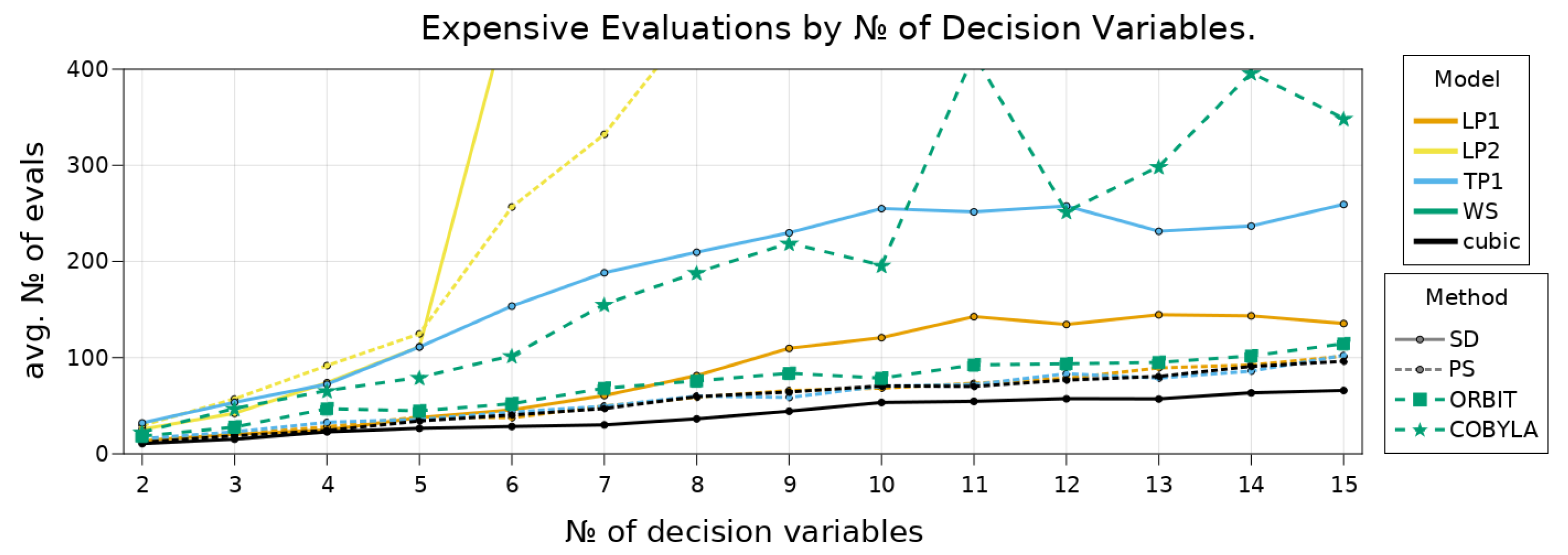
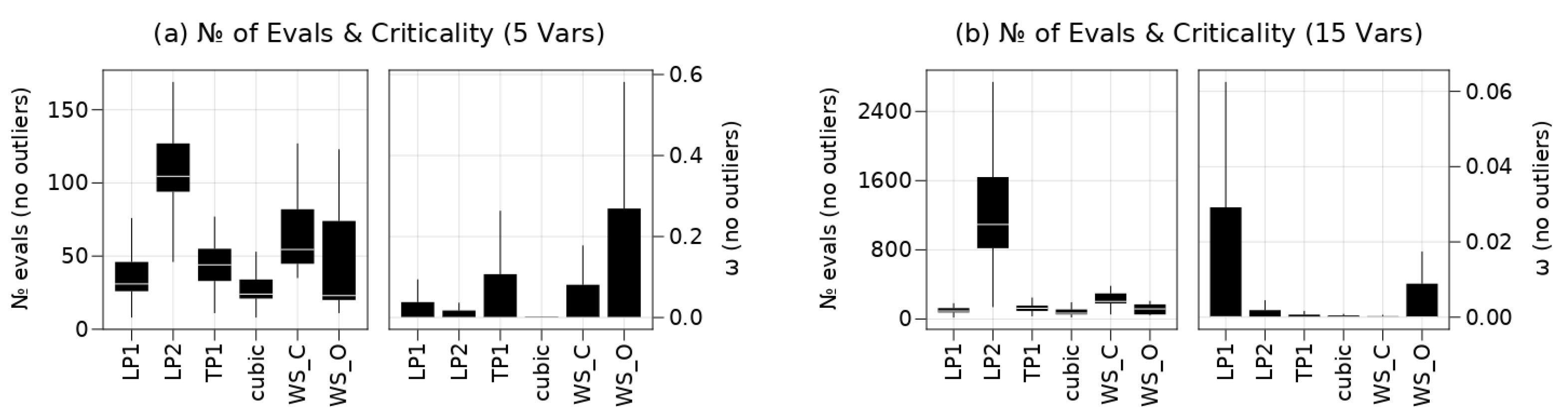
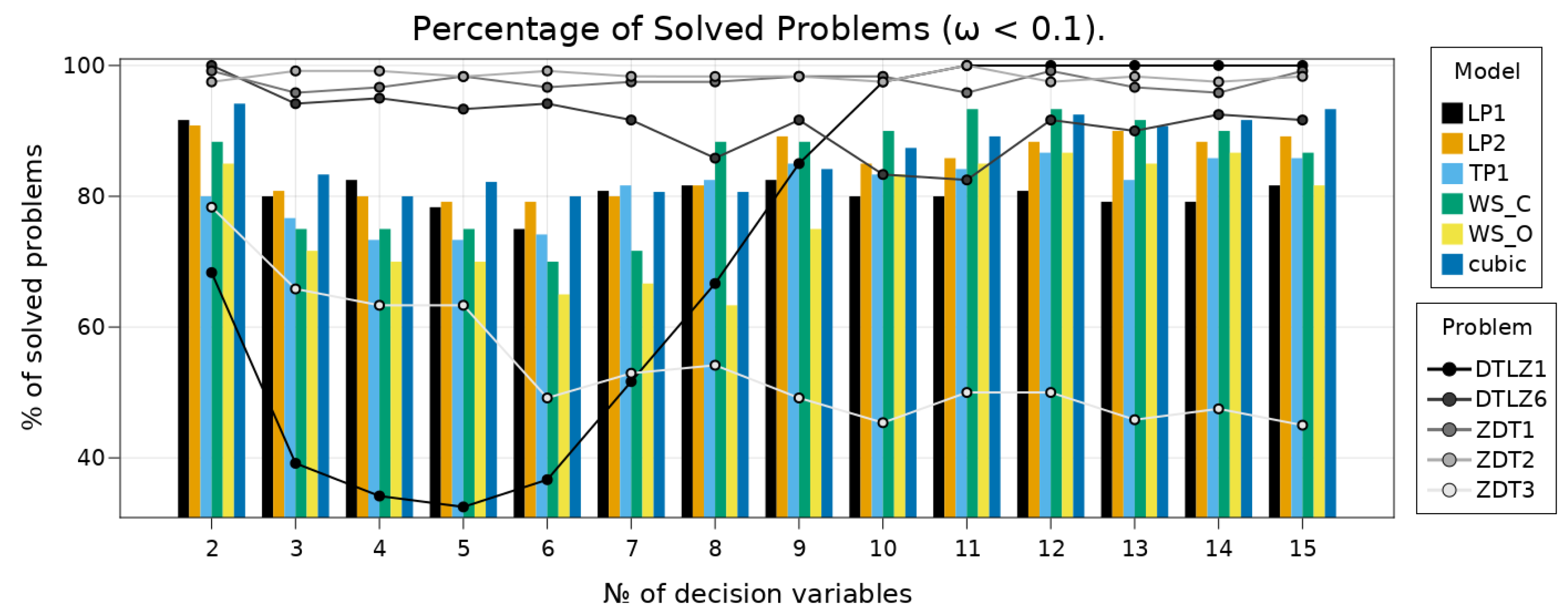
7.3. Benchmarks on Scalable Test-Problems

To assess the performance with a growing number of decision variables n, we performed tests on scalable problems of the ZDT and DTLZ family [51,52]. Figure 3 shows results for the bi-objective problems ZDT1-ZDT3 and for the k-objective problems DTLZ1 and DTLZ6 (we used $k=max\{2,n-4\}$ objectives). All problems are box constrained. Twelve feasible starting points (from the Halton sequence) were generated for each problem setting, i.e., for each combination of n, a test problem and a descent method. The acceptance test and the backtracking were strict.

In all cases the first objective was considered cheap and all other objectives expensive. First and second degree Lagrange models were compared against linear Taylor models and (cubic) RBF surrogates. The Lagrange models were built using a $\Lambda$-poised set, with $\Lambda =1.5$. In the case of quadratic models we used a precomputed set of points for $n\ge 6$. The Taylor models used finite differences and points outside of box constraints were simply projected back onto the boundary. The RBF models were allowed to include up to $(n+1)(n+2)/2$ training points from the database if $n\le 10$ and else the maximum number of points was $2n+1$. Points were first selected from a box of radius ${\theta }_1{\Delta }^{\left(t\right)}$ with ${\theta }_1=2$ and then from a box of radius ${\theta }_2{\Delta }^{\mathrm{ub}}$ with ${\theta }_2=2$. All other parameters differing from the parameters in Table 2 are listed in

Table 3. Parameters for Figure 3, radii relative to ${[0,1]}^n$.

Parameter	${\mathit{\epsilon }}_{\mathbf{crit}}$	${\mathbf{N}}_{\mathbf{it}.}$	${\mathbf{N}}_{\mathbf{exp}.}$	${\mathbf{N}}_{\mathbf{loops}}$	${\Delta }_{\mathbf{crit}}$	${\mathit{\omega }}_{\mathbf{min}}$	${\Delta }_{\mathbf{min}}$	${\mathit{\delta }}_{\mathit{x}}$	${\mathit{\delta }}_{\mathit{f}}$	${\mathit{\nu }}_{+}$	${\mathit{\nu }}_{++}$
Value	${10}^{-2}$	100	$n\times {10}^3$	3	${10}^{-2}$	${10}^{-3}$	${10}^{-6}$	${10}^{-3}$	${10}^{-3}$	0	$0.1$

. The stopping parameters were chosen so as to exit early and save evaluations.

As expected, the second degree Lagrange polynomials require the most objective evaluations and the quadratic dependence on n is clearly visible in Figure 3, and the quadratic growth of the dark-blue line continues for $n\ge 8$. On average, the linear Lagrange models perform better than the linear Taylor polynomials when using the steepest descent steps—also in accordance with our expectations, because only $n+1$ points are needed for each model (versus $2n$ points). Most models—even the linear ones—profit from using the Pascoletti–Serafini subproblems (see Appendix B) over the steepest descent steps. By far the least evaluations (on average) are needed for the RBF models: The black line consistently stays below all other data points. Note, that the RBF models likely appear to perform slightly better with the steepest descent steps because of the early stopping. In other experiments we noticed that RBF models with Pascoletti–Serafini steps can save evaluations when more precise solutions are required.

For comparison, we also used the weighted sum approach with the single objective ${\sum }_{\ell }{f}_{\ell }$ on each problem instance. We tested both the derivative-free COBYLA solver (described in [53] and implemented by NLopt.jl) and the trust region method using steepest descent and cubic RBF models, i.e., our own implementation of ORBIT [34]. Both solvers were restricted to the same number of maximum function evaluations. In fact, ORBIT was configured with the exact same parameters as in Table 3 and the relative stopping tolerances for COBYLA were ${\delta }_x={\delta }_f={10}^{-2}$. Although, COBYLA also uses linear models it requires significantly more evaluations than most other algorithms. The results of the ORBIT scalarization are more comparable to that of the multiobjective runs.

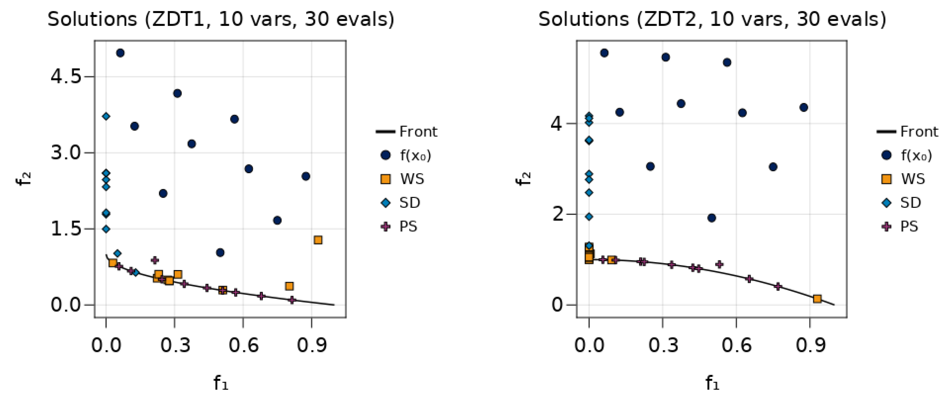
7.3.1. Solution Quality

Figure 4 illustrates that not only do RBF perform better on average, but also overall. With regard to the final solution criticality, there are a few outliers mostly due to DTLZ1 (see also Figure 5). However, in most cases the solution criticality is acceptable, except for the linear Lagrange models. Moreover, Figure 5 shows that a good percentage of problem instances is solved with RBF, especially when compared to the other linear models. Note, that in cases where the true objectives are not differentiable at the final iterate, $\omega$ was set to 0 because the selected problems are non-differentiable only in Pareto optimal points. In Figure 5 it also becomes apparent that the bi-objective DTLZ1 instances were the most challenging for all algorithms. DTLZ1 has many local minima and it is likely to exit early near such a local minimum due to repeated unsuccessful iterations. Likewise, ZDT3 is “flat” towards the true Pareto Front so that it becomes hard to make progress there.

Besides criticality, another metric of interest is the spread of solutions for different starting points. Figure 6 shows the final iterates when the algorithm is applied to the bi-objective problems ZDT1 and ZDT2 for 10 different starting points. Additionally, the problems are solved using the weighted sum approach with the derivative-free COBYLA solver. For each starting point the optimizers were allowed 30 objective evaluations and no data were re-used between runs.

As can bee seen, for these problems, the trust region method readily reaches the critical set using only 30 evaluations. Here, the steepest descent direction tends to generate solutions on the problem boundary when applied in such a global manner—with relatively large trust region radii (${\Delta }^{\left(0\right)}=0.1$ and ${\Delta }^{\mathrm{ub}}=0.5$). Nonetheless, the method remains applicable for local refinement of approximate solutions, e.g., after a coarse search for good starting points using global methods or as a corrector in continuation frameworks. The Pascoletti–Serafini step can be employed with different reference points/directions to provide a better covering than both the steepest descent steps and the weighted sum approach. For Figure 6, the points $\left\{\right[0,-10i],i=1,\dots ,10\}$ were used. The weighted sum approach (with fixed weights) tends to produce clustered solutions. Especially for the non-convex problem ZDT2 only the boundary points of the true Pareto Front are reached, as expected [1].

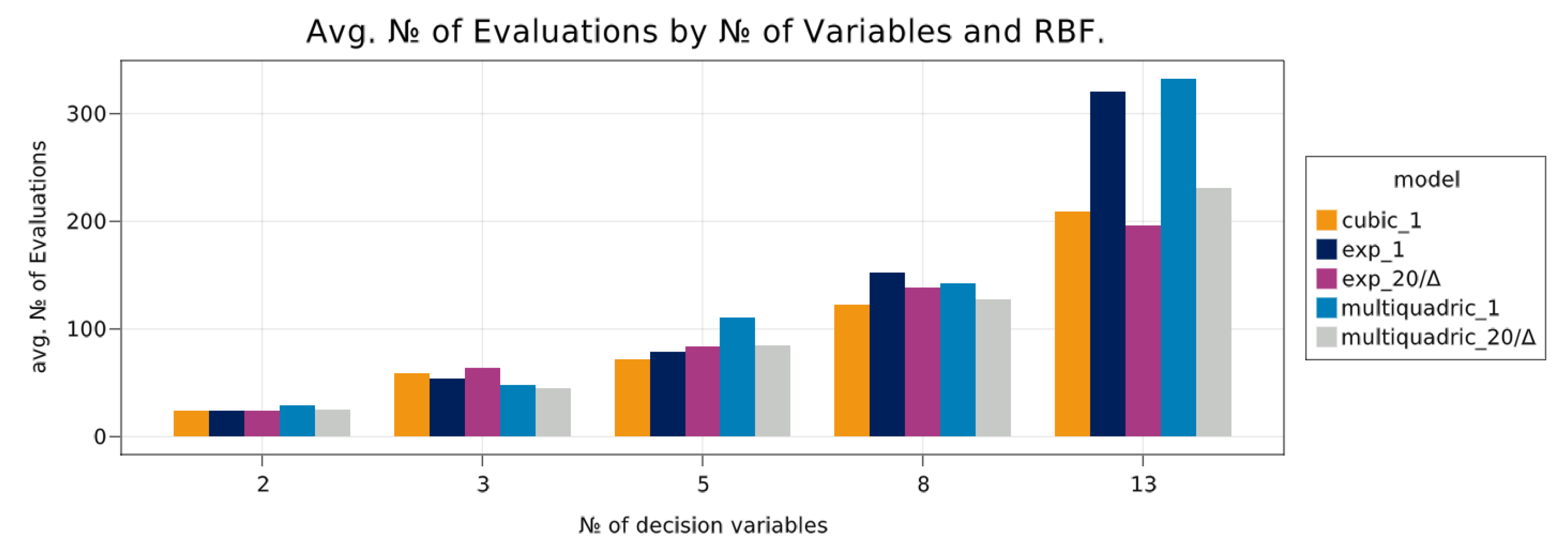
7.3.2. RBF Comparison

Furthermore, we compared the RBF kernels from Table 1. In [34], the cubic kernel performs best on single-objective problems while the Gaussian does worst. As can be seen in Figure 7 this holds for multiple objective functions, too: The Gaussian and the Multiquadric require more function evaluations than the Cubic, especially in higher dimensions. If, however, we use a very simple adaptive strategy to fine-tune the shape parameter, then both kernels can finish significantly faster. In both cases, the shape parameter was set to $\alpha =20/{\Delta }^{\left(t\right)}$ in each iteration. Nevertheless, the cubic function appears to be a good choice in general.

8. Conclusions

We have developed a trust region framework for heterogeneous and expensive multiobjective optimization problems. It is based on similar work [29,30,31,33] and our main contributions are the integration of constraints and of radial basis function surrogates. Subsequently, our method is is provably convergent to first order critical points for unconstrained problems and when the feasible set is convex and compact, while requiring significantly less expensive function evaluations due to a linear scaling of model construction complexity with respect to the number of decision variables.

For future work, several modifications and extensions can likely be transferred from the single-objective to the multiobjective case. For examples, the trust region update can be made step-size-dependent (rather than to depend ${\rho }^{\left(t\right)}$ alone) to allow for a more precise model refinement, see [36] ([Ch. 10]). We have also experimented with the nonlinear CG method [9] for a multiobjective Steihaug–Toint step [36] ([Ch. 7]) and early results look promising.

Going forward, we would like to apply our algorithm to a real world application, similar to what has been done in [54]. Moreover, it would be desirable to obtain not just one but multiple Pareto critical solutions. Because the Pascoletti–Serafini scalarization is still compatible with constraints, the iterations can be guided in image space by providing different global reference points. Furthermore, it is straightforward to use RBF with the heuristic methods from [55] for heterogeneous problems. We believe that it should also be possible to propagate multiple solutions and combine the TRM method with non-dominance testing as has been done [31] and in [56]. One can think of other globalization strategies as well: RBF models have been used in multiobjective Stochastic Search algorithms [57] and trust region ideas have been included into population based strategies [26]. It will thus be interesting to see whether the theoretical convergence properties can be maintained within these contexts by employing a careful trust-region management. Finally, re-using the data sampled near the final iterate within a continuation framework like in [58] is a promising next step.

References

1. Ehrgott, M. Multicriteria Optimization, 2nd ed.; Springer: Berlin, Germany, 2005. [Google Scholar]
2. Jahn, J. Vector Optimization: Theory, Applications, and Extensions, 2nd ed.; Springer: Berlin, Germany, 2011; OCLC: 725378304. [Google Scholar]
3. Miettinen, K. Nonlinear Multiobjective Optimization; Springer: Berlin, Germany, 2013; OCLC: 1089790877. [Google Scholar]
4. Eichfelder, G. Twenty Years of Continuous Multiobjective Optimization. Available online: http://www.optimization-online.org/DB_FILE/2020/12/8161.pdf (accessed on 8 April 2021).
5. Eichfelder, G. Adaptive Scalarization Methods in Multiobjective Optimization; Springer: Berlin, Germany, 2008. [Google Scholar] [CrossRef]
6. Fukuda, E.H.; Drummond, L.M.G. A Survay on Multiobjective Descent Methods. Pesqui. Oper. 2014, 34, 585–620. [Google Scholar] [CrossRef] [Green Version]
7. Fliege, J.; Svaiter, B.F. Steepest descent methods for multicriteria optimization. Math. Method. Operat. Res. (ZOR) 2000, 51, 479–494. [Google Scholar] [CrossRef]
8. Graña Drummond, L.; Svaiter, B. A steepest descent method for vector optimization. J. Comput. Appl. Math. 2005, 175, 395–414. [Google Scholar] [CrossRef] [Green Version]
9. Lucambio Pérez, L.R.; Prudente, L.F. Nonlinear Conjugate Gradient Methods for Vector Optimization. SIAM J. Optim. 2018, 28, 2690–2720. [Google Scholar] [CrossRef]
10. Lucambio Pérez, L.R.; Prudente, L.F. A Wolfe Line Search Algorithm for Vector Optimization. ACM Transact. Math. Softw. 2019, 45, 1–23. [Google Scholar] [CrossRef] [Green Version]
11. Gebken, B.; Peitz, S.; Dellnitz, M. A Descent Method for Equality and Inequality Constrained Multiobjective Optimization Problems. In Numerical and Evolutionary Optimization—NEO 2017; Trujillo, L., Schütze, O., Maldonado, Y., Valle, P., Eds.; Springer: Cham, Switzerland, 2019; pp. 29–61. [Google Scholar]
12. Hillermeier, C. Nonlinear Multiobjective Optimization: A Generalized Homotopy Approach; Springer Basel AG: Basel, Switzerland, 2001; OCLC: 828735498. [Google Scholar]
13. Gebken, B.; Peitz, S.; Dellnitz, M. On the hierarchical structure of Pareto critical sets. J. Glob. Optim. 2019, 73, 891–913. [Google Scholar] [CrossRef] [Green Version]
14. Wilppu, O.; Karmitsa, N.; Mäkelä, M. New Multiple Subgradient Descent Bundle Method for Nonsmooth Multiobjective Optimization; Report no. 1126; Turku Centre for Computer Science: Turku, Sweden, 2014. [Google Scholar]
15. Gebken, B.; Peitz, S. An Efficient Descent Method for Locally Lipschitz Multiobjective Optimization Problems. J. Optim. Theor. Appl. 2021. [Google Scholar] [CrossRef]
16. Custódio, A.L.; Madeira, J.F.A.; Vaz, A.I.F.; Vicente, L.N. Direct Multisearch for Multiobjective Optimization. SIAM J. Optim. 2011, 21, 1109–1140. [Google Scholar] [CrossRef] [Green Version]
17. Audet, C.; Savard, G.; Zghal, W. Multiobjective Optimization Through a Series of Single-Objective Formulations. SIAM J. Optim. 2008, 19, 188–210. [Google Scholar] [CrossRef]
18. Deb, K.; Pratap, A.; Agarwal, S.; Meyarivan, T. A fast and elitist multiobjective genetic algorithm: NSGA-II. IEEE Trans. Evol. Comput. 2002, 6, 182–197. [Google Scholar] [CrossRef] [Green Version]
19. Deb, K. Multi-Objective Optimization Using Evolutionary Algorithms; Wiley: Hoboken, NJ, USA, 2001. [Google Scholar]
20. Coello, C.A.C.; Lamont, G.B.; Veldhuizen, D.A.V. Evolutionary Algorithms for Solving Multi-Objective Problems, 2nd ed.; Springer: New York, NY, USA, 2007. [Google Scholar]
21. Abraham, A.; Jain, L.C.; Goldberg, R. (Eds.) Evolutionary multiobjective optimization: Theoretical advances and applications. In Advanced Information and Knowledge Processing; Springer: New York, NY, USA, 2005. [Google Scholar]
22. Zitzler, E. Evolutionary Algorithms for Multiobjective Optimization: Methods and Applications. Ph.D. Thesis, ETH, Zurich, Switzerland, 1999. [Google Scholar]
23. Peitz, S.; Dellnitz, M. A Survey of Recent Trends in Multiobjective Optimal Control—Surrogate Models, Feedback Control and Objective Reduction. Math. Comput. Appl. 2018, 23, 30. [Google Scholar] [CrossRef] [Green Version]
24. Chugh, T.; Sindhya, K.; Hakanen, J.; Miettinen, K. A survey on handling computationally expensive multiobjective optimization problems with evolutionary algorithms. Soft Comput. 2019, 23, 3137–3166. [Google Scholar] [CrossRef] [Green Version]
25. Deb, K.; Roy, P.C.; Hussein, R. Surrogate Modeling Approaches for Multiobjective Optimization: Methods, Taxonomy, and Results. Math. Comput. Appl. 2020, 26, 5. [Google Scholar] [CrossRef]
26. Roy, P.C.; Hussein, R.; Blank, J.; Deb, K. Trust-Region Based Multi-objective Optimization for Low Budget Scenarios. In Evolutionary Multi-Criterion Optimization; Series Title: Lecture Notes in Computer Science; Deb, K., Goodman, E., Coello Coello, C.A., Klamroth, K., Miettinen, K., Mostaghim, S., Reed, P., Eds.; Springer International Publishing: Cham, Switzerland, 2019; Volume 11411, pp. 373–385. [Google Scholar] [CrossRef]
27. Conn, A.R.; Scheinberg, K.; Vicente, L.N. Introduction to Derivative-Free Optimization; Number 8 in MPS-SIAM Series on Optimization; Society for Industrial and Applied Mathematics/Mathematical Programming Society: Philadelphia, PA, USA, 2009; OCLC: Ocn244660709. [Google Scholar]
28. Larson, J.; Menickelly, M.; Wild, S.M. Derivative-free optimization methods. arXiv 2019, arXiv:1904.11585. [Google Scholar] [CrossRef] [Green Version]
29. Qu, S.; Goh, M.; Liang, B. Trust region methods for solving multiobjective optimisation. Optim. Method. Softw. 2013, 28, 796–811. [Google Scholar] [CrossRef]
30. Villacorta, K.D.V.; Oliveira, P.R.; Soubeyran, A. A Trust-Region Method for Unconstrained Multiobjective Problems with Applications in Satisficing Processes. J. Optim. Theor. Appl. 2014, 160, 865–889. [Google Scholar] [CrossRef]
31. Ryu, J.H.; Kim, S. A Derivative-Free Trust-Region Method for Biobjective Optimization. SIAM J. Optim. 2014, 24, 334–362. [Google Scholar] [CrossRef]
32. Audet, C.; Savard, G.; Zghal, W. A mesh adaptive direct search algorithm for multiobjective optimization. Eur. J. Oper. Res. 2010, 204, 545–556. [Google Scholar] [CrossRef]
33. Thomann, J.; Eichfelder, G. A Trust-Region Algorithm for Heterogeneous Multiobjective Optimization. SIAM J. Optim. 2019, 29, 1017–1047. [Google Scholar] [CrossRef] [Green Version]
34. Wild, S.M.; Regis, R.G.; Shoemaker, C.A. ORBIT: Optimization by Radial Basis Function Interpolation in Trust-Regions. SIAM J. Sci. Comput. 2008, 30, 3197–3219. [Google Scholar] [CrossRef]
35. Conn, A.R.; Scheinberg, K.; Vicente, L.N. Global Convergence of General Derivative-Free Trust-Region Algorithms to First- and Second-Order Critical Points. SIAM J. Optim. 2009, 20, 387–415. [Google Scholar] [CrossRef]
36. Conn, A.R.; Gould, N.I.M.; Toint, P.L. Trust-Region Methods; MPS-SIAM series on optimization; Society for Industrial and Applied Mathematics: Harrisburg, PA, USA, 2000. [Google Scholar]
37. Luc, D.T. Theory of Vector Optimization; Lecture Notes in Economics and Mathematical Systems; Springer: Berlin, Heidelberg, 1989; Volume 319. [Google Scholar] [CrossRef]
38. Thomann, J. A Trust Region Approach for Multi-Objective Heterogeneous Optimization. Ph.D. Thesis, TU Ilmenau, Illmenau, Germany, 2018. [Google Scholar]
39. Nocedal, J.; Wright, S.J. Numerical Optimization, 2nd ed.; Springer Series in Operations Research; Springer: Berlin, Germany, 2006; OCLC: Ocm68629100. [Google Scholar]
40. Wendland, H. Scattered Data Approximation, 1st ed.; Cambridge University Press: Cambridge, UK, 2004. [Google Scholar] [CrossRef]
41. Wild, S.M. Derivative-Free Optimization Algorithms for Computationally Expensive Functions; Cornell University: Ithaca, NY, USA, 2009. [Google Scholar]
42. Wild, S.M.; Shoemaker, C. Global Convergence of Radial Basis Function Trust Region Derivative-Free Algorithms. SIAM J. Optim. 2011, 21, 761–781. [Google Scholar] [CrossRef]
43. Regis, R.G.; Wild, S.M. CONORBIT: Constrained optimization by radial basis function interpolation in trust regions. Optim. Methods Softw. 2017, 32, 552–580. [Google Scholar] [CrossRef]
44. Fleming, W. Functions of Several Variables; Undergraduate Texts in Mathematics; Springer: New York, NY, USA, 1977. [Google Scholar] [CrossRef]
45. Stellato, B.; Banjac, G.; Goulart, P.; Bemporad, A.; Boyd, S. OSQP: An operator splitting solver for quadratic programs. Math. Program. Comput. 2020, 12, 637–672. [Google Scholar] [CrossRef] [Green Version]
46. Johnson, S.G. The NLopt Nonlinear-Optimization Package. Available online: https://nlopt.readthedocs.io/en/latest/ (accessed on 8 April 2021).
47. Svanberg, K. A class of globally convergent optimization methods based on conservative convex separable approximations. SIAM J. Optim. 2002, 12, 555–573. [Google Scholar] [CrossRef] [Green Version]
48. Legat, B.; Timme, S.; Weisser, T.; Kapelevich, L.; Rackauckas, C.; TagBot, J. JuliaAlgebra/DynamicPolynomials.jl: V0.3.15. 2020. Available online: https://zenodo.org/record/4153432#.YG5wjj8RVPY (accessed on 8 April 2021).
49. Runarsson, T.P.; Yao, X. Search biases in constrained evolutionary optimization. IEEE Trans. Syst. Man Cybern. C Appl. Rev. 2005, 35, 233–243. [Google Scholar] [CrossRef] [Green Version]
50. Revels, J.; Lubin, M.; Papamarkou, T. Forward-Mode Automatic Differentiation in Julia. arXiv 2016, arXiv:1607.07892. [Google Scholar]
51. Zitzler, E.; Deb, K.; Thiele, L. Comparison of Multiobjective Evolutionary Algorithms: Empirical Results. Evol. Comput. 2000, 8, 173–195. [Google Scholar] [CrossRef] [Green Version]
52. Deb, K.; Thiele, L.; Laumanns, M.; Zitzler, E. Scalable Test Problems for Evolutionary Multiobjective Optimization. In Evolutionary Multiobjective Optimization; Series Title: Advanced Information and Knowledge Processing; Abraham, A., Jain, L., Goldberg, R., Eds.; Springer: London, UK, 2005; pp. 105–145. [Google Scholar] [CrossRef] [Green Version]
53. Powell, M.J. A direct search optimization method that models the objective and constraint functions by linear interpolation. In Advances in Optimization and Numerical Analysis; Gomez, S., Hennart, J.P., Eds.; Springer: Dordrecht, The Netherlands, 1994; pp. 51–67. [Google Scholar]
54. Prinz, S.; Thomann, J.; Eichfelder, G.; Boeck, T.; Schumacher, J. Expensive multi-objective optimization of electromagnetic mixing in a liquid metal. Optim. Eng. 2020. [Google Scholar] [CrossRef]
55. Thomann, J.; Eichfelder, G. Representation of the Pareto front for heterogeneous multi-objective optimization. J. Appl. Numer. Optim. 2019, 1, 293–323. [Google Scholar]
56. Deshpande, S.; Watson, L.T.; Canfield, R.A. Multiobjective optimization using an adaptive weighting scheme. Optim. Methods Softw. 2016, 31, 110–133. [Google Scholar] [CrossRef] [Green Version]
57. Regis, R.G. Multi-objective constrained black-box optimization using radial basis function surrogates. J. Comput. Sci. 2016, 16, 140–155. [Google Scholar] [CrossRef]
58. Schütze, O.; Cuate, O.; Martín, A.; Peitz, S.; Dellnitz, M. Pareto Explorer: A global/local exploration tool for many-objective optimization problems. Eng. Optim. 2020, 52, 832–855. [Google Scholar] [CrossRef]
Figure 1. (a) Interpolation of a nonlinear function (black) by a Multiquadric surrogate (blue) based on 5 discrete training points (orange). Dashed lines show the kernels and the polynomial tail. (b) Different kernels in 1D with varying shape parameter (1 or 10), see also Table 1.
Mca 26 00031 g001
Figure 2. Two runs with maximum number of expensive evaluations set to 20 (soft limit). Test points are light-gray, the iterates are black, final iterate is red, white markers show other points where the objectives are evaluated. The successive trust regions are also shown. (a) Using Radial Basis Function (RBF) surrogate models we converge to the optimum using only 12 expensive evaluations. (b) Quadratic Lagrange models do not reach the optimum using 19 evaluations. (c) Iterations and test points in the objective space.
Mca 26 00031 g002
Figure 3. Average number of expensive objective evaluations by number of decision variables n, surrogate type and descent method. “SD” refers to steepest descent and “PS” to Pascoletti–Serafini. “LP1” (orange) are linear Lagrange models, “LP2” (yellow) quadratic Lagrange models, “TP1” (blue) are linear Taylor polynomials based on finite differences and “cubic” (black) refers to cubic RBF models. Additionally the results for weighted sum runs are shown in green, using the COBYLA solver and a single objective variant of the trust region framework, ORBIT.
Mca 26 00031 g003
Figure 4. Box-plots of the number of evaluations and the solution criticality for n = 5 and n = 15 for the runs from Figure 3. Outliers are not shown. “WS_C” and “WS_O” refer to the weighted sum approach using COBYLA and ORBIT, respectively.
Mca 26 00031 g004
Figure 5. Each group of bars shows the percentage of solved problem instances, i.e., test runs were the final solution criticality has a value below 0.1. From left to right, the bars correspond to the Trust Region Method (TRM) using linear Lagrange polynomials, the TRM with quadratic Lagrange polynomials, TRM with linear Taylor polynomials, weighted sum with COBYLA, weighted sum with ORBIT and TRM with cubic RBF. Per model and n-value there were 60 runs.
Mca 26 00031 g005
Figure 6. Final iterates in objective space for the bi-objective problems ZDT1 and ZDT2 in 10 variables. The weighted sum method (WS) is compared against the trust region method using steepest descent (DS) and the Pascoletti–Serafini (PS) method.
Mca 26 00031 g006
Figure 7. Each group of bars shows the influence of a adaptive shape radius on the performance of different RBF models (tested on ZDT3) for different decision space dimensions. From left to right the bars correspond to the cubic RBF, the Gaussian—with constant shape factor 1 and with adaptive shape factor 20 / Δ ( t ) —and the Multiquadric—with shape factors 1 and 20 / Δ ( t ) .
Mca 26 00031 g007