Solving Nonholonomic Systems with the Tau Method

Abstract

A numerical procedure based on the spectral Tau method to solve nonholonomic systems is provided. Nonholonomic systems are characterized as systems with constraints imposed on the motion. The dynamics is described by a system of differential equations involving control functions and several problems that arise from nonholonomic systems can be formulated as optimal control problems. Applying the Pontryagins maximum principle, the necessary optimality conditions along with the transversality condition, a boundary value problem is obtained. Finally, a numerical approach to tackle the boundary value problem is required. Here we propose the Lanczos spectral Tau method to obtain an approximate solution of these problems exploiting the Tau toolbox software library, which allows for ease of use as well as accurate results.

1. Introduction

Nonholonomic systems are a class of nonlinear systems that cannot be stabilized by a continuous time-invariant feedback, i.e., at a certain time or state there are constraints imposed on the motion (nonholonomic constraints). These systems are controllable but they cannot move instantaneously in certain directions. They belong to a class of nonlinear differential systems with nonintegrable constraints imposed on the motion [1].

Nonholonomic control systems, which result from formulations of nonholonomic systems that include control inputs, are nonlinear control problems requiring nonlinear treatment. There is ample literature on the formulation of the equations of motion and on the dynamics of nonholonomic systems, being [2] an excellent survey for examples. Nonholonomic control systems have been studied in the context of robot manipulation, mobile robots, wheeled vehicles, and space robotics, just to mention a few. In the case of wheeled vehicles, the kinematics and dynamics can be modeled based on the assumption that the wheels are ideally rolling. Typical constraints of wheeled vehicles are rolling contact, like rolling between the wheels and the ground without slipping, or sliding contact such the sliding of skates.

The solution of nonholonomic optimal control problems can be obtained following a standard procedure, which consists of applying Pontryagin’s maximum/minimum principle to obtain set of equations along with initial and terminal conditions resulting into a two-point boundary value problem (BVP) [3].

In this work we propose the use of the spectral Tau method to obtain approximate solutions of nonholonomic optimal control problems through the associated BVP.

The spectral Tau method produces a polynomial approximation of the solution of the differential problem. It is based on solving a system of linear algebraic equations, obtained by imposing that all conditions are verified exactly and the residual is orthogonal to the first elements of an orthogonal polynomial basis [4].

The paper is organized as follows. Section 2 describes the system model of the nonholonomic wheeled vehicle and Section 3 explains the optimal control formulation. A brief description of the Tau method is presented in Section 4. An illustrative example with numerical results is provided in Section 5 and some conclusions are drawn in Section 6.

2. Nonholonomic Wheeled Vehicle Model

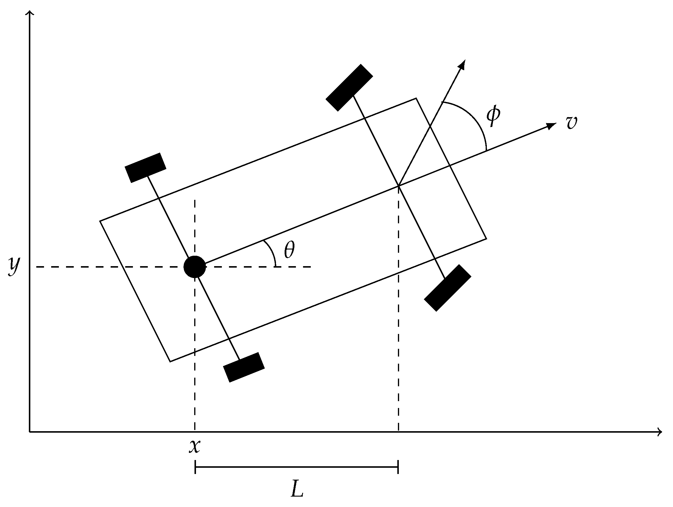
Vehicle models are usually described by a set of ordinary differential equations that define the dynamics of the vehicle and the relationship between the state variables and control input. The kinematic model of a wheeled vehicle can be defined by the following differential equations

$$\begin{array}{c}\dot{x}=f_1(x,y,v,\theta ,\varphi )\hfill \\ \dot{y}=f_2(x,y,v,\theta ,\varphi )\hfill \\ \dot{\theta }=f_3(x,y,v,\theta ,\varphi ),\hfill \end{array}$$

where $(x,y)\in {\mathbb{R}}^2$ is the robot’s position in space, $\theta$ is the angle with respect to the x-axis, $\varphi$ is the steering wheel’s angle with respect to the robot’s longitudinal axis, and v is the velocity. (see Figure 1).

Figure 1. Car-like robot model.

A nonholonomic car-like robot is a car model which rolls without slipping between the wheels and the ground. This constraint is expressed by the equation [5]

$$\dot{x}sin\left(\theta \right)-\dot{y}cos\left(\theta \right)=0.$$

(1)

The simplest model corresponds to a robot with a single wheel: the unicycle model. In this model the wheel rolls on a plane while keeping its body vertical. It is an unrestricted model since it can rotate freely while standing in its position $(x,y)$. Furthermore, the dynamics are characterized by

$$\left\{\begin{array}{c}\dot{x}=vcos\left(\theta \right)\hfill \\ \dot{y}=vsin\left(\theta \right)\hfill \\ \dot{\theta }=\varphi .\hfill \end{array}\right.$$

(2)

The kinematic model of a car-like robot has the same state variables as the unicycle model and its dynamic is represented by

$$\left\{\begin{array}{c}\dot{x}=vcos\left(\theta \right)\hfill \\ \dot{y}=vsin\left(\theta \right)\hfill \\ \dot{\theta }=vu,\hfill \end{array}\right.$$

(3)

where $u\in [-\frac{1}{r},\frac{1}{r}]$ stands for the curvature and r for the turning radius of the robot that corresponds the maximum curvature [6].

3. Optimal Control Problems

An optimal control problem (OCP) can be formulated as

$$\begin{array}{c}{\displaystyle \mathrm{Minimize}J(\mathtt{x}\left(t\right),\mathtt{u}\left(t\right))={\int }_{t_0}^{t_f}F(\mathtt{x}\left(t\right),\mathtt{u}\left(t\right))dt+G(\mathtt{x}\left(t_f\right),t_f)}\hfill \\ \mathrm{subject}\mathrm{to}\hfill \\ \begin{array}{ccc}\hfill & \dot{\mathtt{x}}\left(t\right)=f(\mathtt{x}\left(t\right),\mathtt{u}\left(t\right)),\hfill & t\in [t_0,t_f]\hfill \\ \hfill & \mathtt{x}\left(t_0\right)={\mathtt{x}}_0\hfill \\ \hfill & \mathtt{x}\left(t_f\right)={\mathtt{x}}_f\hfill \\ \hfill & \mathtt{x}\left(·\right)\in X\hfill \\ \hfill & \mathtt{u}\left(·\right)\in U\hfill \\ \hfill & t_f\in [t_0,+\infty [,\hfill \end{array}\hfill \end{array}$$

(4)

where J is the cost function, $\mathtt{x}$ is the state vector representing the dynamics, $\mathtt{u}$ is the control vector, ${\mathtt{x}}_0$ is the initial configuration and ${\mathtt{x}}_f$ is the final configuration.

The solution of the OCP can be obtained following a standard procedure, which consists in applying Pontryagin’s maximum principle and obtaining the necessary optimality conditions along with the transversality condition resulting into a two-point boundary value problem (BVP).

Pontryagin Maximum Principle

Considering the Hamiltonian function

$$H\left(\mathtt{x}\right(t),\mathtt{u}(t),\mathit{\lambda })=F\left(\mathtt{x}\right(t),\mathtt{u}(t\left)\right)+\mathit{\lambda }f\left(\mathtt{x}\right(t),\mathtt{u}(t\left)\right),$$

(5)

where F and f are the functions described above and $\mathit{\lambda }=[{\lambda }_1\left(t\right),{\lambda }_2\left(t\right),\dots ,{\lambda }_n\left(t\right)]$ is a vector of co-state variables, and considering that $(\mathtt{x},{\mathtt{u}}^{*})$ is a controlled trajectory defined over the interval $[t_0,t_f]$ then $(\mathtt{x},{\mathtt{u}}^{*})$ is optimal, for all admissible controls $\mathtt{u}$, if the Pontryagin’s maximum principle holds, i.e.,

$$H(\mathtt{x},{\mathtt{u}}^{*},\mathit{\lambda })\ge H(\mathtt{x},\mathtt{u},\mathit{\lambda }).$$

The Pontryagin maximum principle guarantees that if $(\mathtt{x},{\mathtt{u}}^{*})$ is an optimal pair, a solution of the problem (4), then the first order necessary conditions

$$H_{\mathtt{x}}=-\dot{\mathit{\lambda }}$$

(6)

together with the stationary conditions

$$H_{\mathtt{u}}=0$$

(7)

satisfies the Hamiltonian maximization with transversality conditions given by [3]

$$\begin{array}{cc}\mathit{\lambda }\left(t_f\right)=0\mathrm{if}\hfill & t_f=\infty \mathrm{or}G(.)=0\hfill \\ \mathrm{or}\hfill \\ \mathit{\lambda }\left(t_f\right)={\left.{\displaystyle \frac{\partial G}{\partial \mathtt{x}}}\right|}_{t=t_f}.\hfill \end{array}$$

(8)

This reduces the constrained problem (4) to an unconstrained differential equations system (6)–(8). Usually nonlinear, this system of differential equations can be approximately solved by a numerical method. The next section is devoted to introducing the Tau method, which will be used to numerically tackle the problem.

4. Tau Method

The spectral Tau method produces a polynomial approximation, $y_n\left(x\right)$, of the solution, $y\left(x\right)$, of a given differential problem $Dy\left(x\right)=f\left(x\right)$, satisfying a set of conditions defined on an interval $]a,b[$. Introduced by Lanczos in 1938 [7] to compute approximate solutions of linear differential problems with polynomial coefficients and right-hand side, the Tau method solves a tuned system of linear algebraic equations obtained by imposing that the conditions are verified exactly and that the residual is minimized in a quadrature sense, i.e, is orthogonal to the first elements of an orthogonal polynomial basis. It can be applied, indifferently, to initial, boundary or mixed value problems and it can be implemented with any orthogonal basis. We begin by introducing the method for the original case and then shed some light on how to extend it for the solution of nonlinear problems with non-polynomial coefficients.

4.1. Preliminaries and Notation

Let $\mathbb{P}$ be the space of all algebraic polynomials and let $D:\mathbb{P}\to \mathbb{P}$ be a linear differential operator of order $\nu \ge 1$ with polynomial coefficients represented by

$$D\equiv \sum _{r=1}^{\nu }{p}_r\frac{d^r}{d{x}^r}$$

(9)

and y be the exact solution of the differential problem

$$\left\{\begin{array}{cc}Dy\left(x\right)=f\left(x\right),\hfill & a<x<b\hfill \\ g_j\left(y\right)={\sigma }_j,\hfill & j=1,\dots ,\nu ,\hfill \end{array}\right.$$

(10)

where $f\in \mathbb{P}$ is a polynomial or a convenient polynomial approximation and $g_j$ are $\nu$ linear functionals, acting on $C^{\nu }[a,b]$, representing the (supplementary) conditions.

The main idea of the Tau method is to approximate y by the polynomial $y_n$, solution of the perturbed problem

$$\left\{\begin{array}{cc}D{y}_n\left(x\right)=f\left(x\right)+{\tau }_n\left(x\right),\hfill & a<x<b\hfill \\ g_j\left(y_n\right)={\sigma }_j,\hfill & j=1,\dots ,\nu ,\hfill \end{array}\right.$$

(11)

where ${\tau }_n$ is a polynomial perturbation close to zero in $]a,b[$. Choosing an orthogonal polynomial basis $\mathbf{P}=[P_0,P_1\dots ]$, then the coefficients of $y_n$ are determined imposing that ${\tau }_n$ is orthogonal to $P_i,i=0,1,\dots ,n-\nu$.

The original idea of the Tau method [8] is based on the minimax property of Chebyshev polynomials and on the fact that the solution $y_n$ of (11) depends continuously on the residual ${\tau }_n$. Later generalized to more general bases [4], the method looks for a residual ${\tau }_n$ that minimizes the weighted norm ${\left|\right|.\left|\right|}_w$ associated to the sequence $\mathbf{P}$. Indeed, $\mathbf{P}$ is orthogonal with respect to the weight function $w\left(x\right)$ on $[a,b]$

$$⟨P_i,P_j⟩={\int }_a^{b}w\left(x\right)P_i\left(x\right)P_j\left(x\right)dx=w_i{\delta }_{ij},$$

where $w_i=⟨P_i,P_i⟩=\left|\right|P_i{\left|\right|}_w^2$ and ${\delta }_{ij}$ is the Kronecker delta, and (11) is achieved by imposing

$$⟨{\tau }_n,P_j⟩=0,j=0,1,\dots ,n-\nu ,$$

that is, ${\tau }_n=\mathcal{O}\left(P_{n-\nu }\right)$.

Using suitable matrices, see for example [4,9,10], the differential problem (11) is translated into an algebraic problem. Such matrices must be computed with criteria in order to ensure stable computations [10].

4.2. Nonlinear Problems

Nonlinear differential problems are solved iteratively by first linearizing the problem and then applying the Tau method to the linear inner problem.

Let

$$F\left(y\right)=0,x\in ]a,b[$$

(12)

be a differential equation, where F is a differential operator that could be nonlinear in y and on its derivatives.

From $y_m$, an approximation of the exact solution y, we take the first order Taylor polynomial of F centered in $y_m$ to approximate F

$$D_{m}y=F\left(y_m\right)+\sum _{k=0}^{\nu }(y^{\left(k\right)}-y_m^{\left(k\right)}){\left.\frac{\partial F}{\partial y^{\left(k\right)}}\right|}_{y_m}.$$

(13)

F can be replaced by $D_m$ in (12) to solve

$$\sum _{k=0}^{\nu }{y}^{\left(k\right)}{\left.\frac{\partial F}{\partial y^{\left(k\right)}}\right|}_{y_m}=-F\left(y_m\right)+\sum _{k=0}^{\nu }{y}_m^{\left(k\right)}{\left.\frac{\partial F}{\partial y^{\left(k\right)}}\right|}_{y_m}.$$

(14)

Applying the Tau method to the linear differential Equation (14), an iterative process is implemented to get increasingly better approximations for the differential problem

$$D_m{y}_{m+1}=0,m=0,1,\dots$$

(15)

For additional details on the use of the Tau method for nonlinear problems the reader is invited to read [11].

5. Numerical Experiments

The proposed example is based on the work of [12] and it will be tackled by the Tau method, described in Section 4.

The problem at hand is an optimal control problem of the form (4) with $F=\frac{1}{2}(u_1^2+u_2^2)$ and $G=\frac{1}{2}{\mathbf{x}}^T\left(t_f\right)Q\mathbf{x}\left(t_f\right)$ where $\mathbf{x}$ is the vector of state variables and Q is the weighting matrix.

5.1. System Model

Consider an automated vehicle that moves on a horizontal plane, the contact of each wheel with the floor is assumed to satisfy the rolling without slipping condition and the control inputs are the torque generated by two motors mounted on the wheels. For a fixed final time, it is desired to find the control inputs that minimizes the energy of the final state. This system can be modeled by

$$J=min{\int }_{t_0}^{t_f}\frac{1}{2}(u_1^2+u_2^2)dt+\frac{1}{2}{\mathbf{x}}^T\left(t_f\right)Q\mathbf{x}\left(t_f\right)$$

(16)

subject to

$$\begin{array}{cc}\hfill m\ddot{x}& =\frac{cos\left(\theta \right)}{R}({\mu }_1+{\mu }_2)-\lambda sin\left(\theta \right)\hfill \end{array}$$

(17)

$$\begin{array}{cc}\hfill m\ddot{y}& =\frac{sin\left(\theta \right)}{R}({\mu }_1+{\mu }_2)+\lambda cos\left(\theta \right)\hfill \end{array}$$

(18)

$$\begin{array}{cc}\hfill I\ddot{\theta }& =\frac{L}{R}({\mu }_1-{\mu }_2)\hfill \end{array}$$

(19)

with nonholonomic constraint

$$\dot{x}sin\left(\theta \right)-\dot{y}cos\left(\theta \right)=0,$$

where the position coordinates $(x,y)$, and the heading angle $\theta$, define the system configuration. The mass m, the inertia I, the wheels’ radius R, the half-length of the axis L, are parameters of the system and ${\mu }_1$ and ${\mu }_2$ are torques generated by the motors.

Defining the control inputs $\mathbf{u}={\left[u_1{u}_2\right]}^T$ as

$$u_1=\frac{1}{mR}({\mu }_1+{\mu }_2),u_2=\frac{L}{IR}({\mu }_1-{\mu }_2)$$

and the state variables $\mathbf{x}={\left[x_1{x}_2{x}_3{x}_4{x}_5\right]}^T$ as

$$\begin{array}{cc}\hfill x_1& =xcos\left(\theta \right)+ysin\left(\theta \right)\hfill \\ \hfill x_2& =\theta \hfill \\ \hfill x_3& =-xsin\left(\theta \right)+ycos\left(\theta \right)\hfill \\ \hfill x_4& =\dot{x}cos\left(\theta \right)+\dot{y}sin\left(\theta \right)-\dot{\theta }(xsin\left(\theta \right)-ycos\left(\theta \right))\hfill \\ \hfill x_5& =\dot{\theta }.\hfill \end{array}$$

Equations (17)–(19) can be reduced to the following system of differential equations:

$$\left\{\begin{array}{c}{\dot{x}}_1=x_4\hfill \\ {\dot{x}}_2=x_5\hfill \\ {\dot{x}}_3=-x_1{x}_5\hfill \\ {\dot{x}}_4=-x_1{x}_5^2+u_1+u_2{x}_3\hfill \\ {\dot{x}}_5=u_2.\hfill \end{array}\right.$$

Applying the Hamiltonian H, defined in (5),

$$H(\mathbf{x},\mathbf{u},\mathit{\lambda })=\frac{1}{2}(u_1^2+u_2^2)+\mathit{\lambda }\dot{\mathbf{x}}$$

with $\mathit{\lambda }=\left[{\lambda }_1{\lambda }_2{\lambda }_3{\lambda }_4{\lambda }_5\right]$, and calculating the necessary conditions (6), the stationary conditions (7) and the transversality conditions (8), the following second order system of differential equations is obtained:

$$\begin{array}{c}\hfill \left\{\begin{array}{cc}{x}_1{\dot{x}}_2+{\dot{x}}_3\hfill & =0\hfill \\ {\ddot{x}}_1-{\dot{x}}_2{\dot{x}}_3-{\ddot{x}}_2{x}_3+{\lambda }_4\hfill & =0\hfill \\ {\ddot{x}}_2+x_3{\lambda }_4+{\lambda }_5\hfill & =0\hfill \\ -{\dot{x}}_2{\lambda }_3-{\dot{x}}_2^2{\lambda }_4+{\ddot{\lambda }}_4\hfill & =0\hfill \\ {\ddot{x}}_2{\lambda }_4+{\dot{\lambda }}_3\hfill & =0\hfill \\ -x_1{\lambda }_3+2{\dot{x}}_3{\lambda }_4+{\lambda }_2+{\dot{\lambda }}_5\hfill & =0\hfill \end{array}\right.\end{array}$$

for ${\dot{x}}_1=x_4$, ${\dot{x}}_2=x_5$, ${\dot{\lambda }}_4=-{\lambda }_1$ and ${\dot{\lambda }}_2=0$, with initial and transversality conditions given by

$$\left\{\begin{array}{cc}{x}_i\left(t_0\right)=x_{i0},\hfill & i\in \{1,2,3\}\hfill \\ {\dot{x}}_1\left(t_0\right)=x_{40}\hfill \\ {\dot{x}}_2\left(t_0\right)=x_{50}\hfill \\ {\lambda }_i\left(t_f\right)={\lambda }_{if},\hfill & i\in \{3,4,5\}\hfill \\ {\dot{\lambda }}_4\left(t_f\right)=-{\lambda }_{1f}.\hfill \end{array}\right.$$

(20)

Since this is a nonlinear differential system, in order to implement the Tau method, differential equations need to be linearized. Expressions of the form $uv$ and $u{v}^2$ will be replaced, respectively, by

$$\begin{array}{cc}\hfill uv& \approx v_{m}u+u_{m}v-u_m{v}_m\hfill \\ \hfill u{v}^2& \approx v_m^{2}u+2u_m{v}_{m}v-2u_m{v}_m^2.\hfill \end{array}$$

Thus, the differential system becomes

$$\left\{\begin{array}{cc}{\dot{x}}_{2,m}{x}_1+x_{1,m}{\dot{x}}_2+{\dot{x}}_3\hfill & =x_{1,m}{\dot{x}}_{2,m}\hfill \\ {\ddot{x}}_1-{\dot{x}}_{3,m}{\dot{x}}_2-x_{3,m}{\ddot{x}}_2-{\ddot{x}}_{2,m}{x}_3-{\dot{x}}_{2,m}{\dot{x}}_3+{\lambda }_4\hfill & =-{\dot{x}}_{2,m}{\dot{x}}_{3,m}-{\ddot{x}}_{2,m}{x}_{3,m}\hfill \\ {\ddot{x}}_2+{\lambda }_{4,m}{x}_3+x_{3,m}{\lambda }_4+{\lambda }_5\hfill & =x_{3,m}{\lambda }_{4,m}\hfill \\ ({\lambda }_{3,m}+2{\dot{x}}_{2,m}{\lambda }_{4,m}){\dot{x}}_2+{\dot{x}}_{2,m}{\lambda }_3+{\dot{x}}_{2,m}^2{\lambda }_4+{\ddot{\lambda }}_4\hfill & ={\dot{x}}_{2,m}{\lambda }_{3,m}+2{\dot{x}}_{2,m}^2{\lambda }_{4,m}\hfill \\ {\lambda }_{4,m}{\ddot{x}}_2+{\dot{\lambda }}_3+{\ddot{x}}_{2,m}{\lambda }_4\hfill & ={\ddot{x}}_{2,m}{\lambda }_{4,m}\hfill \\ {\lambda }_{3,m}{x}_1-2{\lambda }_{4,m}{\dot{x}}_3+x_{1,m}{\lambda }_3-2{\dot{x}}_{3,m}{\lambda }_4-{\dot{\lambda }}_5\hfill & =x_{1,m}{\lambda }_{3,m}-2{\dot{x}}_{3,m}{\lambda }_{4,m}+{\lambda }_{2,0}\hfill \end{array}\right.$$

(21)

where $x_{i,m},i=1,2,3$ and ${\lambda }_{i,m},i=3,4,5$ are approximations to $x_1,x_2,x_3$ and ${\lambda }_3,{\lambda }_4,{\lambda }_5$.

The matrix representation of the differential problem (21), together with the conditions (20), is of the form $Ta=b$, where

$$T=\left[\begin{array}{c}C\\ D\end{array}\right]\mathrm{and}b=\left[\begin{array}{c}s\\ f\end{array}\right]$$

with

$$C=\left[\begin{array}{cccccc}\mathbf{P}\left(t_0\right)& 0& 0& 0& 0& 0\\ 0& \mathbf{P}\left(t_0\right)& 0& 0& 0& 0\\ 0& 0& \mathbf{P}\left(t_0\right)& 0& 0& 0\\ {\mathbf{P}}^{\prime }\left(t_0\right)& 0& 0& 0& 0& 0\\ 0& {\mathbf{P}}^{\prime }\left(t_0\right)& 0& 0& 0& 0\\ 0& 0& 0& \mathbf{P}\left(t_f\right)& 0& 0\\ 0& 0& 0& 0& \mathbf{P}\left(t_f\right)& 0\\ 0& 0& 0& 0& 0& \mathbf{P}\left(t_f\right)\\ 0& 0& 0& 0& {\mathbf{P}}^{\prime }\left(t_f\right)& 0\end{array}\right]$$

where $\mathbf{P}\left(t_i\right)=[P_0\left(t_i\right),P_1\left(t_i\right),\dots ]$ represents the action of boundary conditions (20) over the polynomial base elements and ${\mathbf{P}}^{\prime }\left(t_i\right)$ its derivatives. Matrix D represents the differential operator

$$D=\left[\begin{array}{cccccc}{\dot{x}}_{2,m}\left(M\right)& x_{1,m}\left(M\right)N& N& 0& 0& 0\\ N^2& A_{2,2}& A_{2,3}& 0& I& 0\\ 0& N^2& {\lambda }_{4,m}\left(M\right)& 0& x_{3,m}\left(M\right)& I\\ 0& A_{4,2}& 0& -{\dot{x}}_{2,m}\left(M\right)& A_{4,5}& 0\\ 0& {\lambda }_{4,m}\left(M\right)N^2& 0& N& {\ddot{x}}_{2,m}\left(M\right)& 0\\ {\lambda }_{3,m}\left(M\right)& 0& -2{\lambda }_{4,m}\left(M\right)N& x_{1,m}\left(M\right)& -2{\dot{x}}_{3,m}\left(M\right)& N\end{array}\right].$$

Finally,

$$s=[x_{10},x_{20},x_{30},x_{40},x_{50},{\lambda }_{3f},{\lambda }_{4f},{\lambda }_{5f},-{\lambda }_{1f}]$$

$$f=\left[\begin{array}{c}{x}_{1,m}{\dot{x}}_{2,m}\\ -{\dot{x}}_{2,m}{\dot{x}}_{3,m}-{\ddot{x}}_{2,m}{x}_{3,m}\\ x_{3,m}{\lambda }_{4,m}\\ {\dot{x}}_{2,m}{\lambda }_{3,m}+2{\dot{x}}_{2,m}^2{\lambda }_{4,m}\\ x_{1,m}{\lambda }_{3,m}-2{\dot{x}}_{3,m}{\lambda }_{4,m}+{\lambda }_{20}\end{array}\right],$$

where

$$\left\{\begin{array}{c}{A}_{2,2}=-{\dot{x}}_{3,m}\left(M\right)N-x_{3,m}\left(M\right)N^2\hfill \\ A_{2,3}=-{\ddot{x}}_{2,m}\left(M\right)-{\dot{x}}_{2,m}\left(M\right)N\hfill \\ A_{4,2}=({\lambda }_{3,m}\left(M\right)+2{\dot{x}}_{2,m}{\lambda }_{4,m}\left(M\right))N\hfill \\ A_{4,5}=-{\dot{x}}_{2,m}^2\left(M\right)+N^2\hfill \end{array}\right.$$

and M and N are matrices described in [4] representing, respectively, the multiplication and the differentiation operator.

5.2. Numerical Results

In this section we report the numerical results for the example described in Section 5.1 with initial positions $(x,y)=(10,3)$ and heading angle 0. The time interval is $[t_0,f_f]=[0,5]$ and the system parameters used in the simulation are $m=10$ kg, $I=1.2$ kg·m², $R=0.05$ m and $L=0.1$ m. The weighting matrix is $Q=10I$, where I stands for the identity matrix.

The simulation results were obtained using the Tau Toolbox with Chebyshev polynomials.

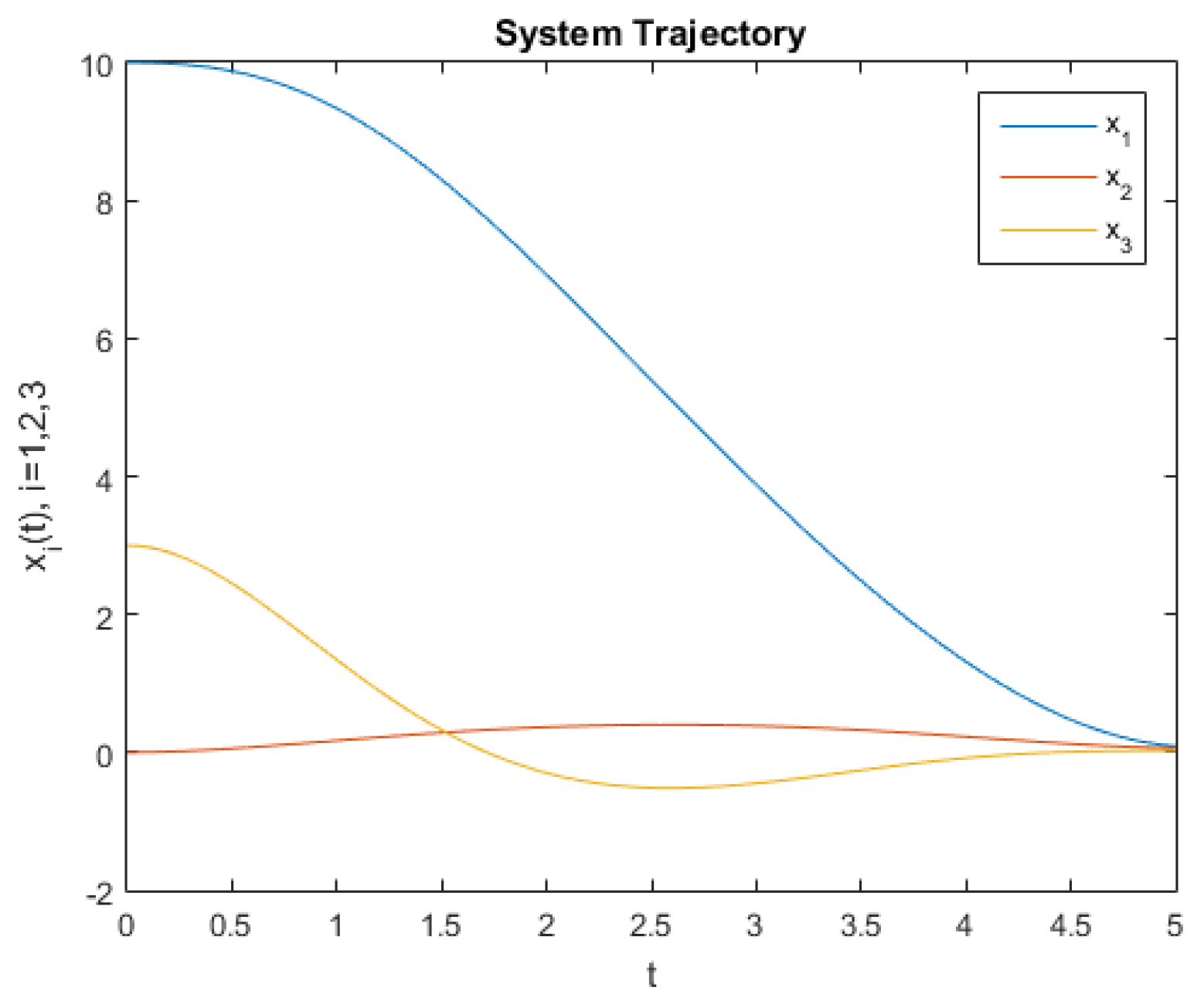
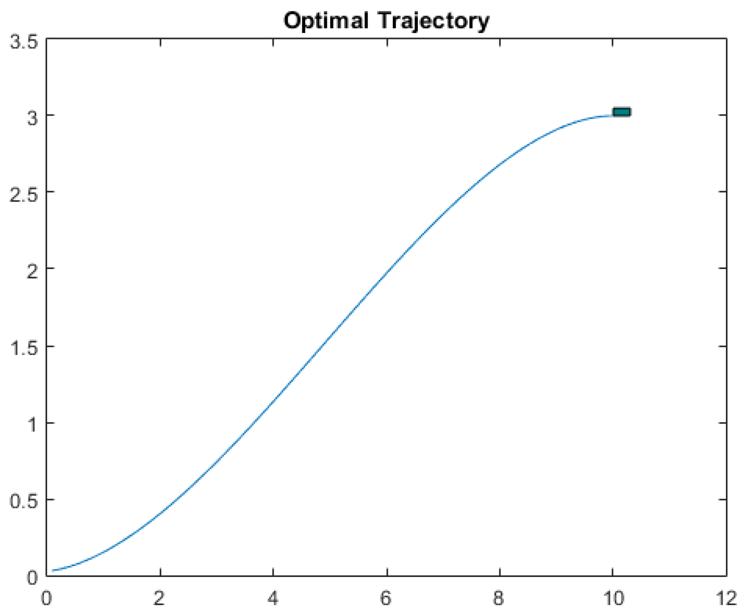
The state trajectories $x_1,x_2$ and $x_3$ and the optimal trajectory for the position $(x,y)$ are illustrated in Figure 2 and Figure 3. The trajectories were obtained with 5th order Chebyshev polynomials.

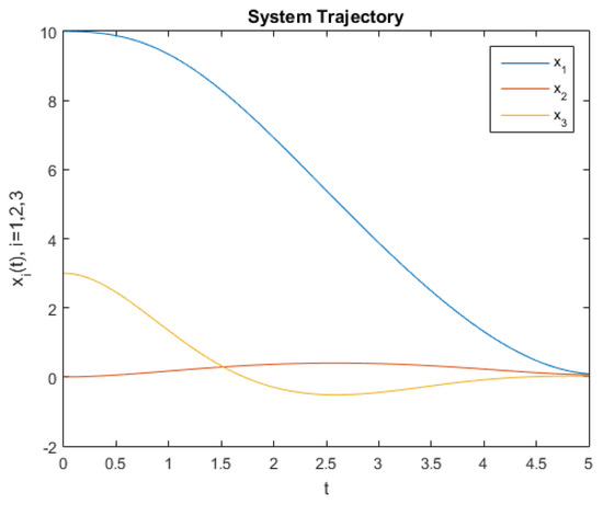
Figure 2. State trajectories $x_1,x_2$ and $x_3$.

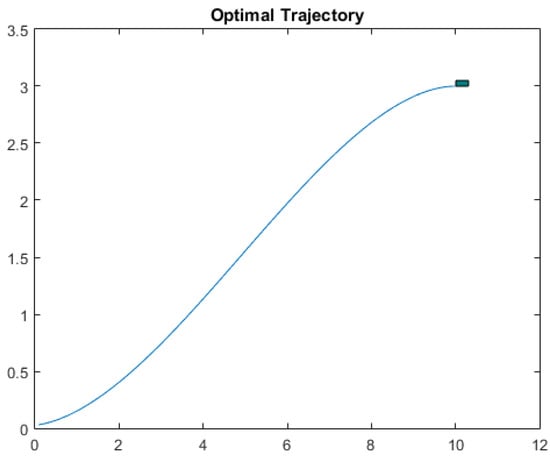
Figure 3. State trajectories $x_1,x_2$ and $x_3$.

These approximate solutions only required $m=8$ iterations to satisfy the stopping criterion $\left|\right|x_i^m-x_i^{m-1}\left|\right|\le {10}^{-14}$. For larger degree polynomials (10 and 15) machine precision can be achieved.

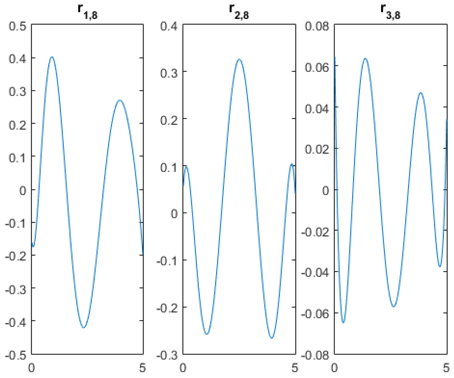
The residual produced by the Tau method in the iteration m is $r_m=D{y}_m$, where $y_m$ is the approximating solution of the system of homogeneous differential equations $Dy=0$. Figure 4 plots the residual $r_{1,m},r_{2,m}$ and $r_{1,m}$ produced by the Tau method for the state variables $x_1,x_2$ and $x_3$, respectively.

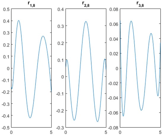
Figure 4. Residual, $r_9=D{y}_9$, produced by the Tau method for the state variables $x_1,x_2$ and $x_3$.

Table 1 presents the values for the functional J defined in (16) using polynomials of degree $n=5,10$ and 15. Since $u_1=-{\lambda }_4\mathrm{and}{u}_2={\dot{x}}_5$, the integral ${\displaystyle {\int }_0^5\frac{1}{2}(u_1^2+u_2^2)dt}$ and $\mathbf{x}{\left(5\right)}^{T}Q\mathbf{x}\left(5\right)$ can be calculated using the the approximate solutions for the state variables $x_i,i=1,\dots ,5$ and the co-state variable ${\lambda }_4$.

Table 1. J values for several polynomial degree approximations.

Polynomial Degree	Functional Value
5	5.0990
10	5.0878
15	5.0880

As the polynomial multiplication and differentiation, the integration can be set into algebraic operation as well, using a suitable matrix [4].

6. Conclusions

The Lanczos spectral Tau method was used to compute approximate polynomial solutions for nonholonomic systems. A detailed illustration on the approximation procedure is offered. The Tau toolbox provides the appropriate environment to solve systems of ordinary differential problems while allowing for accurate solutions, whenever the sought solution is regular. Numerical results for this dynamical optimization problem confirm both aspects: ease of use and accuracy of approximation.

References

- Fontes, F.A.C.C. Discontinuous feedbacks, discontinuous optimal controls, and continuous-time model predictive control. Int. J. Robust Nonlinear Control IFAC Affil. J. 2003, 13, 191–209. [Google Scholar] [CrossRef]
- Kolmanovsky, I.; McClamroch, N.H. Developments in nonholonomic control problems. IEEE Control Syst. Mag. 1995, 15, 20–36. [Google Scholar]
- Athans, M.; Falb, P.L. Optimal Control: An Introduction to the Theory and Its Applications; Courier Corporation: North Chelmsford, MA, USA, 2007. [Google Scholar]
- Ortiz, E.L.; Samara, H.J. An operational approach to the Tau method for the numerical solution of non-linear differential equations. Computing 1981, 27, 15–25. [Google Scholar] [CrossRef]
- Angeles, J.; Kecskemethy, A. Kinematics and Dynamics of Multi-Body Systems; Springer: Berlin, Germany, 2014. [Google Scholar]
- De Luca, A.; Oriolo, G.; Samson, C. Feedback control of a nonholonomic car-like robot. In Robot Motion Planning and Control; Springer: Berlin, Germany, 1998; pp. 171–253. [Google Scholar]
- Coleman, J. The Lanczos tau-method. IMA J. Appl. Math. 1976, 17, 85–97. [Google Scholar] [CrossRef]
- Lanczos, C. Trigonometric interpolation of empirical and analytical functions. J. Math. Phys. 1938, 17, 123–199. [Google Scholar] [CrossRef]
- Trindade, M.; Matos, J.; Vasconcelos, P.B. Towards a Lanczos’Tau-method toolkit for differential problems. Math. Comput. Sci. 2016, 10, 313–329. [Google Scholar] [CrossRef]
- Vasconcelos, P.; Matos, J.; Trindade, M. Spectral Lanczos’ Tau Method for Systems of Nonlinear Integro-Differential Equations. In Integral Methods in Science and Engineering; Constanda, C., Dalla Riva, M., Lamberti, P., Musolino, P., Eds.; Birkhäuser: Cham, Switzerland, 2017; Volume 1, pp. 305–314. [Google Scholar]
- Gavina, A.; Matos, J.; Vasconcelos, P.B. Improving the Accuracy of Chebyshev Tau Method for Nonlinear Differential Problems. Math. Comput. Sci. 2016, 10, 279–289. [Google Scholar] [CrossRef]
- Yih, C.C.; Ro, P.I. Near-optimal motion planning for nonholonomic systems using multi-point shooting method. In Proceedings of the IEEE International Conference on Robotics and Automation, Minneapolis, MN, USA, 22–28 April 1996; Volume 4, pp. 2943–2948. [Google Scholar]
© 2019 by the authors. Licensee MDPI, Basel, Switzerland. This article is an open access article distributed under the terms and conditions of the Creative Commons Attribution (CC BY) license (http://creativecommons.org/licenses/by/4.0/).