Abstract
This paper considers three dynamic systems composed of a mathematical pendulum suspended on a sliding body subjected to harmonic excitation. A comparative dynamic analysis of the studied parametric mutations of the rigid pendulum with inertial suspension point and damping was performed. The examined system with parametric mutations is solved numerically, where phase planes and Poincaré maps were used to observe the system response. Lyapunov exponents were computed in two ways to classify the dynamic behavior at relatively early stage of forced responses using two proven methods. The results show that with some parameters three systems exhibit a very similar dynamic behavior, i.e., quasi-periodic and even chaotic motions.
1. Introduction
Mechanical engineering or other fields always require elaboration based on numerical computations. Each mechanical system associated with periodic excitation behaves unpredictably. Excitations can come from the internal imperfections of the system, such as parametric asymmetry, eccentricity or external forces such as wind, road defects, etc. Any chaotic behavior is undesirable, and their consequences can lead to the destruction of the system. One method of qualitative determination of the state of the system is based on computations of Lyapunov exponents. Qualitatively, it informs about the form of the dynamic response of the system.
These exponents are certain characteristic numerical values, creating a spectrum that helps in the qualitative assessment of the dynamics of the system. They determine the convergence or divergence of infinitely close trajectories that begin close to each other. To know the nature of system dynamics, all we need to know is the sign of the Lyapunov exponent λ defined as follows:
The Lyapunov exponent in Equation (1) is denoted by λ. Any positive value in the limit accounts for chaos in the system, while non-positive proves the regularity.
There are many numerical methods of computing Lyapunov exponents, e.g., Wolf method, Rosenstein method, Kantz method, method based on neural network modification, synchronization method, and others, see [1,2,3,4,5,6]. There are two main approaches to numerical assessment in the literature: with known motion equations and a time series approach. For example, the first method of computing the full spectrum of Lyapunov exponents is presented in [3], the calculation of the largest Lyapunov exponent is given in [5,6], and the determination of the spectrum of Lyapunov exponents can be found in [7].
From a practical point of view, Lyapunov exponents are used in various fields of science, such as: rotor systems [8], electricity systems [9], aerodynamics [10].
2. The Parametric Pendulum and Its Mutations
Figure 1 shows the three analyzed dynamical systems. The first system presented in Figure 1a is a mathematical pendulum of the length attached to the moving slider of the point-focused mass . The inertial slider moves horizontally back and forth along the x-axis and is subjected to harmonic forcing , where denotes amplitude of the force, and states the frequency of forcing. In the second system depicted in Figure 1b the pendulum of the length is replaced by a parametric pendulum, the length of which is described by the function , where is the amplitude of the periodic change of the length about . The generalized coordinates of first and second systems are: the angle between the pendulum and vertical axis and the displacement of the slider. In the third system shown in Figure 1c the first rigid pendulum of constant length is replaced by an elastic form, where and describe linear stiffness and damping, respectively. The generalized coordinates for the third system can be noted: dynamical elongation of the spring, the angle between the pendulum and vertical axis and the displacement of the slider.
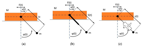
Figure 1.
The analyzed systems: (a) rigid pendulum, (b) first parametric mutation, (c) second parametric mutation in an elastic form.
In order to simplify mathematical modelling of the problem the following assumptions are made:
- there is no friction in the inertial slider;
- masses of the pendulum’s swinging body and slider are treated as point-focused masses;
- pendulum arm of a constant or variable length is massless.
Dynamical analysis of the system mutations is preceded by derivation of equations of motion. To find them, one can use Newton laws, however, this approach requires a better knowledge of the system. A more universal and simpler approach bases on deriving them from the Euler–Lagrange equation [11].
2.1. Mathematical Model of Rigid Pendulum
The kinetic energy of the analyzed two-degrees-of-freedom (2 DoF) system is the sum of kinetic energies of the slider () and the pendulum ():
In the assumed configuration of the model the potential energy of the analyzed system is as follows:
Referring to Figure 1, the following denotations have been used in Equations (2) and (3): —mass of the sliding body, —mass of the mathematical pendulum, —linear displacement and —velocity of the sliding body, —angular displacement and —angular velocity of the pendulum, —constant length of the rigid pendulum (Figure 1a), —gravitational constant.
The Lagrangian satisfies the Euler–Lagrange equation for any of the assumed generalized coordinates. Therefore, one writes:
Substituting the Equations (2) and (3) for the kinetic and potential energy into the Lagrangian, respectively, it allows to derive the equation of motion for each of the generalized coordinates. The number of coupled equations of motion depends on the number of generalized coordinates. The equations of motion for the analyzed 2 DoF system are as follows:
- for the generalized coordinate φ (pendulum angle):
- for the generalized coordinate x (displacement of the slider):
The equations of motion (5)–(6) can be algebraically decoupled with respect to the second derivate:
2.2. Mathematical Model of First Mutation of the Rigid Pendulum
The kinetic energy of the analyzed two-degree-of-freedom model with parametric pendulum is equal to the sum of the kinetic energy of the slider and kinetic energy of the pendulum body:
The potential energy of the analyzed system is as follows:
The Lagrangian satisfies the Euler–Lagrange equation for any of the assumed generalized coordinates. Therefore, one writes:
From Equation (10) one can obtain two equations of motion:
- for the generalized coordinate φ (pendulum angle):
- for the generalized coordinate x (displacement of the slider):
And after decoupling Equations (11) and (12) with respect to the second derivative:
2.3. Mathematical Model of the Second Mutation of the Rigid Pendulum
Similar derivation for the three-degree-of-freedom system was performed in [12]. The equation for kinetic energy was found follows:
The potential energy of the analyzed system is equal to the potential energy of the pendulum body and potential energy of the spring:
The generalized form of the Euler–Lagrange equation for the third case is as follows:
and R is Rayleigh dissipation function:
The equations of motion have the following form:
- for the generalized coordinate s (pendulum elongation):
- for the generalized coordinate φ (pendulum angle):
- for the generalized coordinate x (displacement of the slider):
Equations (18)–(20) can be algebraically decoupled with respect to the second derivate:
3. Methods
To numerically solve the systems of second order ordinary differential Equations (7), (13) and (21), they were written in the form of first order differential equations. The vector of initial conditions for the first and second system is assumed, . In the case of the third system of three degrees of freedom, the additional equation associated with the pendulum elongation only represents the incremental elongation of the spring measured from its free length . The vector of initial conditions is assumed as well, Numerical analysis of the presented models was carried out in two different environments. Phase planes and Poincaré maps were found using a program prepared in the Python programming language, and computations of Lyapunov exponents were carried out using codes written in Matlab environment. ODEINT from the SciPy Python library and ODE45 from the Matlab library was used to solve the system of ordinary differential equations.
Computation of Lyapunov Exponents
Lyapunov exponents are one of the most commonly used tools in analyzing the impact of small disturbances on system solution. These are the values that determine the exponential convergence or divergence of trajectories beginning close to each other [13].
Two methods of computing Lyapunov exponents were used in the study. The first method is described in [14]. This method simultaneously solves the first-order ODE system, its variational equations and determines the spectrum of Lyapunov exponents. The second method used for computations is available on the Mathworks file sharing page [15]. The numerical code is based on the algorithm for computing Lyapunov exponents on the basis of ODE proposed in the work [4].
Both selected methods were validated for the Lorenz system written in Equation (22) with the parameters , , and and also initial conditions . Table 1 shows a comparison of obtained Lyapunov exponents spectrum with a reference values found in [16]:

Table 1.
Comparison of Lyapunov exponents (time is measured in seconds).
Computed spectra of Lyapunov exponents are very similar to the reference values taken from the literature [13,14], respectively.
4. Results
Presented systems were examined for the set of parameters presented in Table 2.
Table 2.
Parameters of the simulations (values of , , and are common for all the systems).
Frequency of harmonic forcing was assumed in the range from to rad/s. Vector of state variables for the first and second system is assumed, , and for the third system is taken as follows, = .
4.1. Numerical Simulation of the Rigid Pendulum
Figure 2, Figure 3, Figure 4 and Figure 5 show phase planes and Poincaré maps for different frequencies of harmonic excitation . By the assumed definition, the map definition results in stroboscopic analysis of the phase space at time instances being a multiple of the period . The map presentation on a shaded background created by a cross-section of the phase space has most likely been first used in the work [17]. The corresponding values of Lyapunov exponents are shown in Table 3.
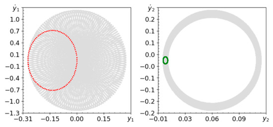
Figure 2.
Phase planes (gray lines) and Poincaré maps (red and green dots) for ω = 3.64.
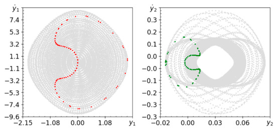
Figure 3.
Phase planes (gray lines) and Poincaré maps (red and green dots) for ω = 4.94.
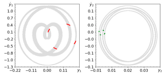
Figure 4.
Phase planes (gray lines) and Poincaré maps (red and green dots) for ω = 7.24.
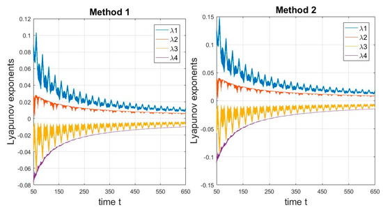
Figure 5.
Time history of Lyapunov exponents for ω = 4.94 (the case of rigid pendulum)
Table 3.
Spectra of Lyapunov exponents for the system with rigid pendulum.
As shown in the Poincaré maps in Figure 2, Figure 3 and Figure 4, a system with a rigid pendulum of constant length tends to be quasi-periodic. For the tested ω∈[1.24, 9.24] rad/s with a step of 0.1, the system is stable and does not show chaotic behavior (in a vibration that is far from a resonance frequency of excitation). However, forms of quasi-periodic behavior change with frequency, but do not stabilize on periodic orbits. The computed spectra of Lyapunov exponents indicate that the behavior of the system is two-periodic. Lyapunov exponents and tend to converge to zero, while the others are negative. Both methods provide slightly different but similar results. Interesting trajectories of the convergence of Lyapunov exponents are presented in Figure 5.
The and exponents stabilize, while and oscillate with decreasing amplitude, which was necessary to prove. The behavior of a rigid pendulum with a fixed length can be compared with the behavior of the third system with a flexible pendulum with assumed damping constant.
4.2. Numerical Simulation of the First Mutation of the Rigid Pendulum
Selected behaviors of the dynamical model of two degrees of freedom with a parametric forcing are presented in Figure 5, Figure 6 and Figure 7. Table 4 shows the computed spectra of Lyapunov exponents.
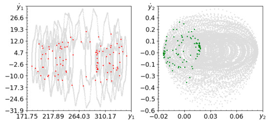
Figure 6.
Phase planes (gray lines) and Poincaré maps (red and green dots) for A = 0.1, ω = 4.94.
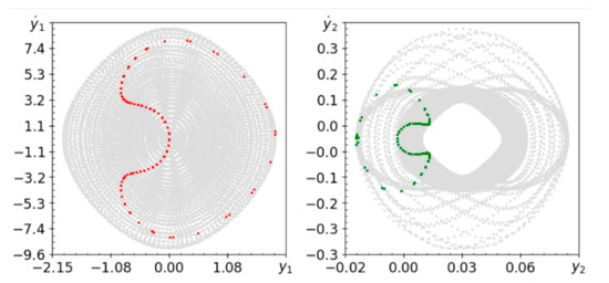
Figure 7.
Phase planes (gray lines) and Poincaré maps (red and green dots) for A = 0.1, ω = 7.64.
Table 4.
Spectra of Lyapunov exponents for the first mutation of rigid pendulum.
Replacing a rigid pendulum with a fixed length by a parametric pendulum makes the system more unpredictable.
The system is not able to achieve periodic behavior for the frequencies tested. Figure 6 shows chaotic or quasi-periodic behavior, but the definitely positive value of Lyapunov exponents confirms the chaotic behavior of the system. Figure 8 presents the time history of the Lyapunov exponents spectrum. You can see that the exponents are stable and the system is chaotic. The system may also exhibit quasi-periodic behavior, as shown in Figure 7. Amplitude of periodic change in length of about has a significant impact on the behavior of the system. When the value varies from to , and the harmonic forcing frequency increases by about , the system exhibits chaotic behavior, as shown in Figure 9. Such behavior can easily be seen on the Poincaré map and this is clearly indicated by definitely positive Lyapunov exponent. By changing parameter , quasi-periodic or chaotic behavior is observed in different frequency ranges.
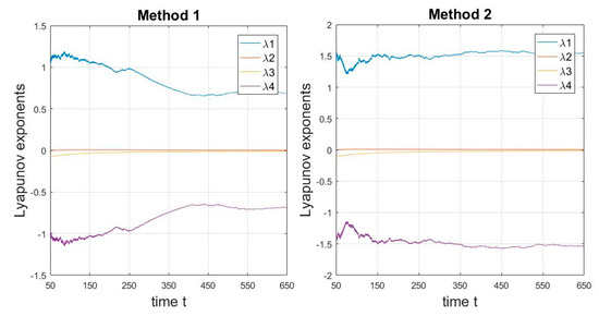
Figure 8.
Time history of Lyapunov exponents for .
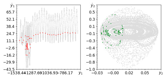
Figure 9.
Phase planes (gray lines) and Poincaré maps (red and green dots) for , .
4.3. Numerical Simulation of the Second Mutation of Rigid Pendulum
In Figure 10, Figure 11 and Figure 12 phase planes and Poincaré maps for the second mutation are presented. Table 5 presents the computed spectra of Lyapunov exponents.
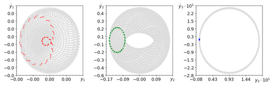
Figure 10.
Phase planes (gray lines) and Poincaré maps (red, green and blue dots) for , and .
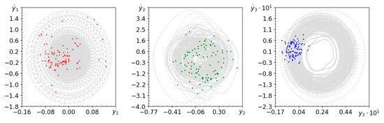
Figure 11.
Phase planes and Poincaré maps (colors as above) for , and .
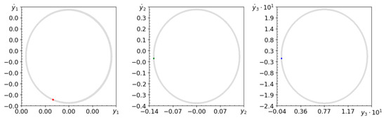
Figure 12.
Phase planes and Poincaré maps (colors as above) for , and .
Table 5.
Spectra of Lyapunov exponents for the system with second mutation of rigid pendulum.
In the case of a system with a flexible pendulum, it is worth noting the effect of damping. In the case of weak damping and low frequency of harmonic forcing, the system shows quasi-periodic behavior, as shown in Figure 10.
Figure 11 shows that at higher forcing frequencies the system remains chaotic. Strong damping makes the system stiffer, and some weak damping gives the system more freedom. This hypothesis was verified in Figure 12, on which periodic movement is clearly visible. Numerical analysis showed that for , where , behaviors are periodic. The computed values of Lyapunov exponents (see Table 5) confirm the observed dynamic behavior. Figure 13 proves that for quasi-periodic motion, the spectrum of Lyapunov exponents changes with an increasingly smaller amplitude. Figure 14 shows that in the case of periodic conservation and high energy dispersion in the system spectra of Lyapunov exponents are more stable than in the case of quasi-periodicity.
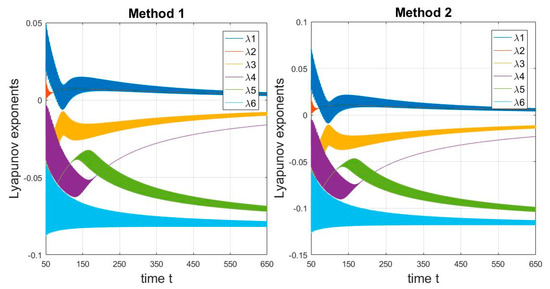
Figure 13.
Time history of Lyapunov exponents starting at for , , .
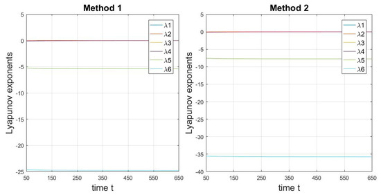
Figure 14.
Time history of Lyapunov exponents starting at for , k = 40 and .
4.4. Observation of Similarities in the Behaviour of Systems with a Rigid Pendulum and Its Mutations
In this section, we present the results for a special case when all the analyzed systems behave in a similar way. In the case of the second system, the amplitude of the pendulum length is A = 0.001, while the parameters of the third system are as follows, k = 2000 and C = 0.05.
The previously presented spectra of Lyapunov exponents have proved that the most accurate results are obtained for a longer observation time, therefore in this part only the results for time are presented.
Figure 15, Figure 16 and Figure 17 show the behavior of the second system, while the spectrum of Lyapunov exponents can be found in Table 6.
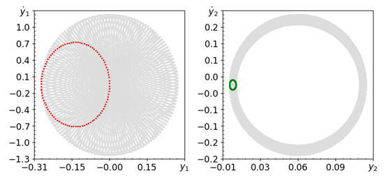
Figure 15.
Phase planes (gray lines) and Poincaré maps (red and green dots) for , .
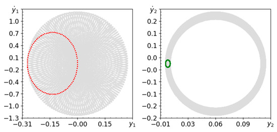
Figure 16.
Phase planes and Poincaré maps (colors as above) for , .
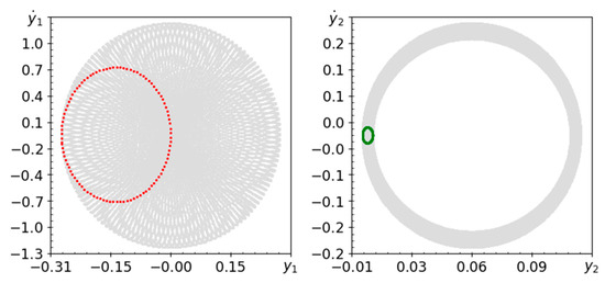
Figure 17.
Phase planes and Poincaré maps for , .
Table 6.
Spectra of Lyapunov exponents for the second mutation of the system with rigid pendulum.
For a small amplitude of pendulum length changes, the behavior of the system is the same as for a rigid pendulum system.
Figure 15, Figure 16 and Figure 17 show quasi-periodic behavior because they show almost the same behavior as Figure 2, Figure 3 and Figure 4. The values of Lyapunov exponents in Table 3 and Table 6 are very close to each other. This means that with a small change in the length of the pendulum, the second system with the first mutation of the pendulum behaves as rigid.
Figure 18, Figure 19 and Figure 20 show the results for a system with a flexible parametric pendulum. The corresponding spectra of Lyapunov exponents can be found in Table 7.
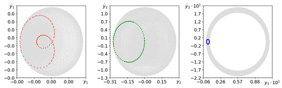
Figure 18.
Phase planes (gray dots) and Poincaré maps (red, green and blue dots) , and .
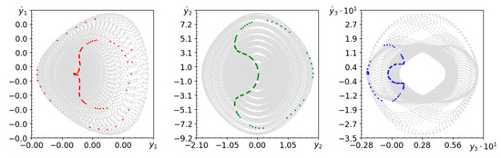
Figure 19.
Phase planes and Poincaré maps (colors as above) for , and .
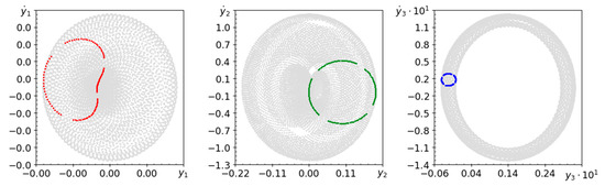
Figure 20.
Phase planes and Poincaré maps (colors as above) for , and .
Table 7.
Spectra of Lyapunov exponents for the system with elastic pendulum.
In the case of very high stiffness and low damping of the parametric pendulum, the behavior of the system is usually quasi-periodic. Phase planes and Poincaré maps presented in Figure 18, Figure 19 and Figure 20 are very similar to those shown in Figure 2, Figure 3 and Figure 4. This means that the behavior of a system with a parametric elastic pendulum is almost the same as that of a rigid counterpart. The computed spectra of Lyapunov exponents indicate quasi-periodic behavior.
Visible differences may be due to early stage dynamics, where both methods may have different convergence factors to the most true values. However, we note that despite this, the type of behavior observed has been verified.
5. Conclusions
Mathematical models of the system with inertial sliding body, rigid pendulum and its parametric mutations were created. The dynamics of the three systems were examined on the basis of phase planes, Poincaré maps and spectra of Lyapunov exponents. It was observed that the first system consisting of a fixed-length pendulum and an inertial slider behaves quasi-periodically. The results for the second system show that the behavior of the system strongly depends on the amplitude of the periodic change in length around its static elongation. For small pendulum length amplitudes, the behavior is quasi-periodic or chaotic, but if the amplitude is high enough, the system tends to be chaotic, as confirmed by Lyapunov exponents. As for the system containing the parametric pendulum, it has been observed that for the same value of pendulum stiffness the behavior of the system depends on the amount of dispersed kinetic energy. In the case of small values of the damping coefficient, the system easily behaves chaotically, while in the case of high values of the coefficient, it behaves periodically.
If the amplitude of the pendulum length change around the static elongation for the second system is very small, the system behaves almost the same as a rigid pendulum system. A similar conclusion can be drawn by comparing the behavior of the third system (the second parametric mutation of the pendulum) with the first system. For high elastic pendulum stiffness value and low damping factor the observed behaviors are similar.
Selected methods of computing Lyapunov exponents gave rather similar results and proved to be very useful. The behavior of the examined models based on the obtained values of Lyapunov exponents are consistent with the results obtained from the Poincaré map visualization. It has been observed that for the periodic and chaotic movement, the values of Lyapunov exponents appear to stabilize over time. In the case of quasi-periodic behavior of the spectral system of Lyapunov exponents, they fluctuate with decreasing amplitude.
Author Contributions
Conceptualization, P.O.; methodology, W.Ś. and T.L. and P.O.; software, P.O., W.Ś.; validation, W.Ś. and P.O.; formal analysis, W.Ś. and P.O.; investigation, W.Ś. and T.L. and P.O.; resources, P.O.; data curation, W.Ś. and T.L.; writing—W.Ś. and P.O.; writing—review and editing, P.O.; visualization, W.Ś. and T.L. and P.O.; supervision, P.O.; project administration, W.Ś. and T.L.
Acknowledgments
The work was carried out in 2018–2019 as part of the “Research Problem Based Learning” project at the Faculty of Mechanical Engineering at the Lodz University of Technology.
Conflicts of Interest
The authors declare no conflicts of interest.
References
- Awrejcewicz, J.; Krysko, A.V.; Erofeev, N.P.; Dobriyan, V.; Barulina, M.A.; Krysko, V.A. Quantifying chaos by various computational methods. Part 1: Simple systems. Entropy 2018, 20, 175. [Google Scholar] [CrossRef]
- Awrejcewicz, J.; Krysko, A.V.; Erofeev, N.P.; Dobriyan, V.; Barulina, M.A.; Krysko, V.A. Quantifying chaos by various computational methods. Part 2: Vibrations of the Bernoulli–Euler beam subjected to periodic and colored noise. Entropy 2018, 20, 170. [Google Scholar] [CrossRef]
- Benettin, G.; Galgani, L.; Giorgilli, A.; Strelcyn, J.-M. Lyapunov exponents for smooth dynamical systems and hamiltonian systems; a method for computing all of them, part I: Theory, part II: Numerical application. Meccanica 1980, 15, 21–30. [Google Scholar] [CrossRef]
- Wolf, A.; Swift, J.B.; Swinney, H.L.; Vastano, J.A. Determining Lyapunov exponents from a time series. Nonlinear Phenom. 1985, 16, 285–317. [Google Scholar] [CrossRef]
- Pikunov, D.; Stefanski, A. Numerical analysis of the friction-induced oscillator of Duffing’s type with modified LuGre friction model. J. Sound Vib. 2019, 440, 23–33. [Google Scholar] [CrossRef]
- Stefanski, A.; Dabrowski, A.; Kapitaniak, T. Evaluation of the largest Lyapunov exponent in dynamical systems with time delay. Chaos Solit. Fractals 2005, 23, 1651–1659. [Google Scholar] [CrossRef]
- Sano, M.; Sawada, Y. Measurement of the Lyapunov spectrum from a chaotic time series. Phys. Rev. Lett. 1985, 55, 1082–1085. [Google Scholar] [CrossRef] [PubMed]
- Xiang, L.; Deng, Z.; Hu, A.; Gao, X. Multi-fault coupling study of a rotor system in experimental and numerical analyses. Nonlinear Dyn. 2019, 97, 2607–2625. [Google Scholar] [CrossRef]
- Wadduwage, D.P.; Wu, C.Q.; Annakkage, U.D. Power system transient stability analysis via the concept of Lyapunov exponents. Electr. Power Syst. Res. 2013, 104, 183–192. [Google Scholar] [CrossRef]
- Hu, D.L.; Liu, X.B.; Chen, W. Moment Lyapunov exponent and stochastic stability of binary airfoil under combined harmonic and Gaussian white noise excitation. Nonlinear Dyn. 2017, 89, 539–552. [Google Scholar] [CrossRef]
- Awrejcewicz, J. Classical Mechanics Dynamics; Springer: Berlin, Germany, 2012. [Google Scholar]
- Pietrzak, P.; Ogińska, M.; Krasuski, T.; Figueiredo, K.; Olejnik, P. Near the resonance behavior of a periodicaly forced partially dissipative three-degrees-of-freedom mechanical system. Lat. Am. J. Solids Struct. 2018, 15, 1–12. [Google Scholar] [CrossRef]
- Balcerzak, M.; Pikunov, D.; Dabrowski, A. The fastest, simplified method of Lyapunov exponents spectrum estimation for continuous-time dynamical systems. Nonlinear Dyn. 2018, 94, 3053–3065. [Google Scholar] [CrossRef]
- Van Wyk, M.A.; Steeb, W.-H. Chaos in Electronics; Kluwer Academic Publishers: Dordrecht, The Netherlands, 1997. [Google Scholar]
- Calculation Lyapunov Exponents for ODE. Available online: https://www.mathworks.com/matlabcentral/fileexchange/4628-calculation-lyapunov-exponents-for-ode (accessed on 15 October 2019).
- Ramasubramanian, K.; Sriram, M.S. A comparative study of computation of Lyapunov spectra with different algorithms. Phys. D 2000, 139, 72–86. [Google Scholar] [CrossRef]
- Awrejcewicz, J.; Olejnik, P. Stick-slip dynamics of a two-degree-of-freedom system. Int. J. Bifurc. Chaos 2003, 13, 843–861. [Google Scholar] [CrossRef]


© 2019 by the authors. Licensee MDPI, Basel, Switzerland. This article is an open access article distributed under the terms and conditions of the Creative Commons Attribution (CC BY) license (http://creativecommons.org/licenses/by/4.0/).