Abstract
CO2 capture attracts significant research efforts in order to reduce the volume of greenhouse gases emitted from fossil fuels combustion. Among the studied processes, chemical absorption represents a mature approach and, in this direction, new solvents, alternatives to monoethanolamine (MEA), have been suggested. In this work, the solubility of CO2 in aqueous solutions of 2-amino-2-methyl-1-propanol (AMP) and 3-(methylamino)propylamine (MAPA), which were recently suggested as constituents of novel phase change solvent mixtures, is experimentally measured at 298, 313, 323, and 333 K and in a wide range of pressures, up to approximately 7 bar. As the available literature experimental data for MAPA aqueous solutions are very limited, the experimental results of this study were compared to respective literature data for AMP, and a very satisfactory agreement was observed. The new experimental data were correlated with the cubic-plus-association (CPA) and the modified Kent-Eisenberg models. It was observed that both models rather satisfactorily correlate the experimental data, with the Kent-Eisenberg model presenting more accurate correlations.
Keywords:
CO2 capture; alkanolamines; chemical absorption; phase equilibria; CPA; Kent-Eisenberg model; AMP; MAPA 1. Introduction
Global temperatures have risen by approximately 1 °C since pre-industrial times [1]. It is believed that greenhouse gases, such as carbon dioxide, nitrous oxide, methane, and others, have a high impact on global warming, and CO2 emissions due to fossil fuels combustion are considered as the primary anthropogenic contribution factor [2]. They are mainly relevant to power plants, which contribute approximately 40% of the globally emitted CO2 [3]. The present CO2 annual emissions are estimated around 36 billion tons, compared to 2 billion tons in 1900 [4], and this figure is projected to drastically increase over the next decades if considerable measures are not taken. Such predicted increase of CO2 emissions is affected by several factors of high uncertainty, including technological aspects and economic growth, but may be limited by CO2 climate policies.
In this direction, the CO2 capture from flue gases has attracted significant research interest, and a variety of processes have been suggested, such as chemical and physical absorption, surface adsorption, chemical looping combustion, membrane separation, cryogenic, and others [5]. The strengths and weaknesses of such processes have been investigated from technical, economic, and social points of view in several studies, as noted in recent review articles [1,2,5]. However, chemical absorption using liquid solvents is considered as the most mature technology, as it is broadly used for removing acid gases form natural gas and can be easily retrofitted onto existing plants [6]. Nevertheless, if applied to existing power plants that utilize fossil fuels, it significantly increases the electricity cost, mainly due to the high energy (heat) demands for the regeneration of the solvent [6,7]. Consequently, increased research efforts have focused on efficient solvent systems, which are alternatives to the conventionally used aqueous monoethanolamine (MEA) solutions, and which include phase change solvents [8], new alkanolamines and their mixtures [9,10], deep eutectic solvents, and ionic liquids [5]. Nevertheless, amines represent the most studied family of solvents for CO2 capture applications.
CO2 absorption in aqueous solutions of primary and secondary amines follows two distinct chemical pathways: CO2 hydration and carbamate formation [11,12]. CO2 aqueous chemistry can be fully described by the following reactions:
Formation of bicarbonate ion:
Dissociation of bicarbonate ion:
Ionization of water:
The reaction of the first amine molecule ( with results in the formation of a zwitterion intermediate (, which, subsequently, forms a carbamate ( through the removal of a proton by a second amine molecule. Then, the carbamate can be hydrolized into bicarbonate.
Zwitterion formation:
Carbamate formation:
Carbamate hydrolysis:
The formation of a stable carbamate, which results in low absorption capacity (1 mole of per 2 moles of amine), is mainly dependent on the structure of the amine molecule. In the case of unhindered primary and secondary alkanolamines, such as monoethanolamine (MEA), the carbamate formation is favored because the hydrolysis reaction occurs only to a minor extent. However, the carbamate of hindered amines, such as AMP, is usually unstable and, consequently, the main product is the bicarbonate [13]. Hence, the overall reactions involving unhindered (Equation (7)) and hindered amines (Equation (8)) can be expressed as follows:
Unhindered amines:
Hindered amines:
From reactions (7) and (8), it follows that the maximum loading for unhindered amines is stoichiometrically limited to 0.5 mole of per mole of amine, whereas for hindered ones it is equal to 1 mole of per mole of amine. However, despite the fact that sterically hindered primary and secondary amines present higher CO2 loading values, they usually show lower reaction rates [8,14].
In this work, aqueous mixtures of 2-amino-2-methyl-1-propanol (AMP) and 3-(methylamino)propylamine (MAPA) are investigated. Their structures are shown in Figure 1. AMP is considered as a sterically hindered amine, whereas MAPA is a diamine containing one primary and one secondary amine group. Both were suggested as constituents of novel phase change solvent systems, which usually are aqueous solutions of amine mixtures that exhibit liquid–liquid (VLLE) phase separation upon increase of temperature. The phase split of such solvent systems allows the regeneration of only the CO2 rich phase, which is usually the aqueous one, resulting in decreased energy demands [8,9,14]. In this direction, Zhang suggested the addition of AMP in a phase change aqueous N,N-dimethylcyclohexyl amine (DMCA)-N-methylcyclohexyl amine (MCA) mixtures [14], as the addition of AMP increases the lower critical solution temperature above 40 °C, without compromising the absorption or desorption performance of the phase-change solvent [14]. Subsequently, the phase behavior of such system was investigated by Tzirakis et al., who also screened the absorption ability of several phase change solvents [15], including aqueous DMCA–MAPA mixtures [16]. However, the most studied MAPA containing phase change solvent is the aqueous DEEA–MAPA system, which was suggested by Pinto et al. [17]. In such solvent systems, ΜAPA is used as an absorption activator, according to the classification suggested by Zhang [14], as it exhibits high CO2 solubility and fast kinetics.
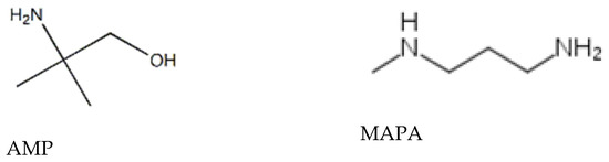
Figure 1.
Structure of AMP and MAPA.
The use of both AMP and MAPA in novel solvent systems, as well as the suggestion of AMP as potential alternative to MEA, revealed the need for accurate experimental data. The available literature studies containing data for the CO2 solubility in pure MAPA and AMP aqueous solutions are shown in Table 1 and Table 2, respectively. Nevertheless, the use of both AMP and MAPA in novel solvent systems with a more complex phase behavior (VLLE) than the phase behavior of conventional alkanolamine aqueous solutions (VLE) reveals the need for accurate thermodynamic models that are capable of successful prediction of the phase behavior. This, however, implies the need of accurate experimental data, even on systems containing fewer of the relevant compounds, for the effective parameterization of the models.
The rigorous thermodynamic modeling of such highly non-ideal multicomponent systems requires accounting for all intermolecular interactions, including the ionic interactions among the various species. This can be only performed using electrolyte models, such as the electrolyte EoS/GE models, or various electrolyte equation of state (EoS) theories, considering also the equilibrium constants of all chemical reactions [18,19,20]. Nevertheless, such an approach presents significant complexity, and usually several simplifications are applied. Considering the use of equation of state models, the most popular simplification is not to explicitly account for chemical interactions, but to effectively account for them through the hydrogen bonding term of the relevant models [9,21,22,23,24]. Such a pseudo-chemical reaction approach was used by Rodriguez et al., who applied the SAFT-VR model to calculate the absorption of CO2 in aqueous amine solutions [21]. More recently, the SAFT-γ equation of state was used, showing successful predictions for the loading of CO2 in amine solutions and their phase behavior [9,22]. In the same direction, Tzirakis at al. [24] and Leontiadis et al. [23] used the SRK-CPA EoS, whereas Wang et al. [25] used the PR-CPA, for correlating the solubility of CO2 in aqueous amine solutions. The thermodynamic routes for modeling the acid gases solubility in aqueous amine solutions were recently reviewed [25].

Table 1.
Literature studies reporting experimental data for the CO2 solubility in aqueous MAPA solutions.
Table 1.
Literature studies reporting experimental data for the CO2 solubility in aqueous MAPA solutions.
| Temperature (K) | Composition | Reference |
|---|---|---|
| 313, 333, 353, 373 | 8 m | Chen et al. [26] |
| 313, 353, 393 | 1, 2 M | Arshad et al. [10] |
| 313, 333, 353, 373 | 8 m | Voice et al. [27] |
Table 2.
Literature studies reporting experimental data for the CO2 solubility in aqueous AMP solutions.
Table 2.
Literature studies reporting experimental data for the CO2 solubility in aqueous AMP solutions.
| Temperature (K) | Composition | Reference |
|---|---|---|
| 313, 393 | 3 M | Sartori and Savage [13] |
| 313, 373 | 2, 3 M | Roberts and Mather [28] |
| 323 | 3.43 M | Teng and Mather [29] |
| 313, 343 | 2 M | Teng and Mather [30] |
| 293, 313, 333, 353 | 2, 3 M | Tontiwachwuthikul et al. [31] |
| 301, 303, 313, 323, 333, 343, 353 | 2 M | Haji-sulaiman and Aroua [32] |
| 303 | 2 M | Haji-sulaiman et al. [33] |
| 313 | 2 M | Jane and [34] |
| 313, 333, 353 | 2.43, 2.44, 2.45, 6.14, 6.24, 6.48 mol/kg | Silkenbäumer et al. [35] |
| 313, 333, 353 | 30 wt. % | Park et al. [36] |
| 303, 313, 323 | 2, 2.8, 3.4 M | Kundu et al. [37] |
| 313, 333, 353, 373, 393 | 3 M | Tobiesen et al. [38] |
| 323 | 15, 30 wt. % | Arcis et al. [39] |
| 313 | 3 M | Yang et al. [40] |
| 298, 308, 318, 328 | 2.5, 3.4, 4.9 mol/dm3 | Dash et al. [41] |
| 303, 313, 333 | 1, 2, 3 M | Sharrif et al. [42] |
| 313, 333, 353, 373 | 30 wt. % | Tong et al. [43] |
| 313, 333, 363 | 2 M | Nordin et al. [44] |
| 313, 333, 353, 373 | 3.4 M, 30 wt. % | Tong et al. [45] |
| 373, 393, 413, 433 | 4.8 M | Li et al. [46] |
| 313 | 2.5 M | Nouacer et al. [47] |
| 318 | 3 M | Kortunov et al. [48] |
| 313, 333, 363 | 2 M | Narku-Tetteh et al. [49] |
| 313, 333, 353 | 0.1, 1, 3 M | Hartono et al. [50] |
Nevertheless, it was found that empirical approaches, which are considerably simpler, result in very satisfactory correlations for the solubility of acid gases in aqueous amine solutions. The most popular one is probably the Kent-Eisenberg model, which requires knowledge of the equilibrium constants for all chemical reactions [51]. In its original form, the literature values of Henry’s law and ionization constants were used, except from those referring to the amine ionization reaction and the carbamate hydrolysis, which were adjusted to experimental solubility data. The effective values of the adjustable parameters absorb all non-idealities of the system, resulting in very satisfactory results [52]. Consequently, the model found many applications in correlating the acid gases solubility in aqueous amine and alkanolamine solutions and several modifications appeared in literature, which were recently reviewed [53].
In this work, the equilibrium solubility of CO2 in aqueous AMP (17.7% wt.) and MAPA (30.0% wt.) solutions was experimentally measured, using a pressure decay method, over the temperature range of 298–333 K and CO2 partial pressures up to approximately 7 bar. The new experimental data for AMP and MAPA were used to parameterize the CPA equation of state model, which was used for the first time to such amine containing systems. The Kent-Eisenberg model was also used to correlate the CO2 solubility in the aqueous solutions, using new parameters, estimated in this study.
2. Experimental Setup
2.1. Materials
The materials used are shown in Table 3. They were used as received without further purification.
Table 3.
Chemicals used in this work.
2.2. Experimental Apparatus and Procedure
The applied pressure decay method and the experimental apparatus, which is shown in Figure 2, are described in detail by Leontiadis et al. [23]. The equilibrium cell (high pressure stainless steel with internal volume of 152.2 ± 1.6 cm3 at 25 °C) is equipped with a pressure transducer (WIKA A-10, ±0.5%) and a Pt-100 thermometer (±0.01 K). The cell is immersed into a water bath (model Grant TC-120, temperature stability of 0.1 K). When the entire assembly reaches the desired temperature, a measured (weighted with accuracy of 0.001 g) amount of the solvent is fed into the equilibrium cell, which is evacuated, so the solvent exists under its own vapor pressure. After that, a known (weighted, maximum error ±0.005 g) amount of gas is introduced into the cell using a needle valve. The equilibrium is confirmed when the pressure in the cell remains constant for at least 1 h. At this point the pressure is recorded.
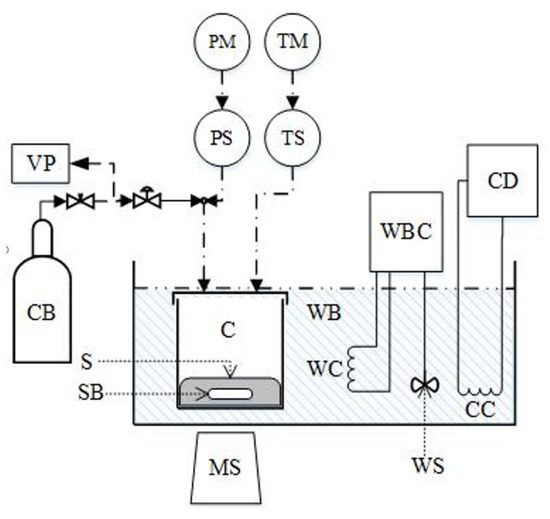
Figure 2.
Experimental apparatus for VLE measurements consisting of: equilibrium cell (C), solution (S) weighted CO2 flask (CB), cooling coil (CC), cooling device (CD), magnetic stirrer (MS), pressure indicator (PM), pressure sensor (PS), stirring bar (SB), temperature indicator (TM), Pt-100 thermometer (TS), vacuum pump (VP), water bath (WB), temperature controller/heater (WBC), heating coil (WC), and stirrer (WS). Reproduced from [23], with permission from Elsevier.
As the CO2 densities, which were obtained from NIST [54], the total mass of CO2, the volume of the cell, and the pressure of system are known, the absorbed amount of CO2 is calculated. According to such procedure, the total pressure of the cell is measured. The CO2 partial pressure is estimated through subtraction of the solution’s vapor pressure from the total pressure. Such approximation is very often used in similar pressure decay studies [10,23,24,55]. Because the investigated solutions present very low vapor pressures, such correction is insignificant, especially at relatively high pressures (higher than 1 bar).
3. Theory
3.1. The Cubic Plus Association (CPA) Equation of State
The cubic plus association (CPA) equation of state is a combination of a cubic equation of state (the SRK model was used in this study) with the hydrogen bonding term of the SAFT type models that is based on the Wertheim’s first order thermodynamic perturbation theory [56]. In terms of pressure, P, it can be expressed as follows [57,58]:
where xi is the mole fraction of component i and XAi is the fraction of the free (not associated with other active sites) A-sites on molecule i, which is related to the association strength ΔAiBj through the following equation:
The association strength, ΔAiBj, between two sites, A on molecule i and site B on molecule j, is:
where is the radial distribution function, the reduced density, ρ the molar density, εAiBj the association energy, βAiBj the association volume, and . The co-volume parameter, bi, of component i is considered temperature independent.
A Soave-type relation is used for the interaction energy of the physical term, as follows:
where a0 and c1 are pure fluid parameters and Tr is the reduced temperature.
The association energy, εAiBj, and the association volume, βAiBj, that are shown in Equation (11) are only used for associating components, and, along with the three parameters of the physical term (αο, b, c1), are the five pure fluid parameters of the model.
In this study, the conventional mixing rules were used in the physical (SRK) term for the interaction energy and co-volume, using one binary interaction parameter, kij, as shown by the next relations:
To account for cross association interactions between two self-associating compounds (e.g., between water and amines) the CR-1 rule [59], described by the following relations, was used:
In addition, the modified CR-1 rule was used to account for cross-association (solvation) interactions between one self- and one non-self-associating fluid [59]:
3.2. The Kent-Eisenberg Model
The chemical equilibrium in the systems comprising CO2, alkanolamines (primary or secondary) and water can be fully described by the following set of reactions [11,12]:
Protonation of amine
Hydrolysis of carbamate
Formation of bicarbonate ion
Dissociation of bicarbonate ion
Ionization of water
where and denote the protonated form of the amine () and the carbamate anion, respectively.
The Kent-Eisenberg model sets all activity coefficients equal to unity [51], thus the relevant equilibrium constants are written as follows:
Henry’s law relates the equilibrium partial pressure to the dissolved concentration in the liquid phase as follows:
Overall mass balances and charge equations can be written as follows:
Amine balance:
CO2 balance:
Charge balance:
The equilibrium constants of Equations (22)–(26), the Henry’s law relationship presented in Equation (27), and the material and charge balances (Equations (28)–(30)) can be reduced to a single fifth-order polynomial equation in terms of the concentration of hydrogen ions, [60]. Thus, for carbamate forming amine solutions, the following fifth-order polynomial equation is obtained [53]:
where parameters A, B, C, D, E, and F are shown in Table 4.
Table 4.
Parameters of Equation (31).
Only the root with physical meaning, i.e., , is kept from Equation (31) [60]. Then, the CO2 loading is calculated through the following equations [53]:
where:
For non-carbamate forming amines, such as AMP, reaction (18) can be neglected because no carbamates are formed. Thus is omitted in material and charge balances (Equations (28)–(30)) resulting in the following fourth-order polynomial equation [60]:
where parameters A, B, C, D, and E are shown in Table 5.
Table 5.
Parameters of Equation (34).
Consequently, the total CO2 loading () can be calculated through the following equation [53]:
In both cases, i.e., for carbamate and non-carbamate forming amines, the equilibrium constants , as well as the Henry’s law constant, , are estimated through the following empirical relation [53]:
4. Results and Discussion
4.1. Experimental Results
CO2 loading measurements were performed at 298, 313, 323, and 333 K and various pressures for aqueous solutions that contain AMP (17.7% wt., approximately 2.0 M) and MAPA (30.0% wt., approximately 3.36 M). The obtained experimental data for the AMP and MAPA solutions are presented in Table 6 and Table 7, respectively. The reported uncertainties in the loading values denote the maximum error, calculated through propagation of errors, considering the uncertainties in the weight of the materials added in the equilibrium cell, in the volume of the cell, in densities, etc.
Table 6.
CO2 solubility in 17.7% wt. (2 M) AMP aqueous solutions at 298–333 K a.
Table 7.
CO2 solubility in 30.0% wt. (3.36 M) MAPA aqueous solutions at 298–333 K a.
The new data of this study are illustrated in Figure 3, Figure 4, Figure 5 and Figure 6 and Figure 7, Figure 8, Figure 9 and Figure 10 for AMP and MAPA, respectively. They are compared with available literature experimental data. As it is presented in Figure 3, Figure 4, Figure 5 and Figure 6 and in Table 2, there are some literature experimental data for 2 M aqueous AMP solutions at 313, 323, and 333 K, but it was not possible to find literature data for 298 K. On the other hand, it was not possible to find literature experimental data for 30% wt. aqueous MAPA solutions. Comparisons of Figure 4, Figure 5 and Figure 6 show a rather satisfactory agreement between the new data obtained in this work and the available experimental data from literature.
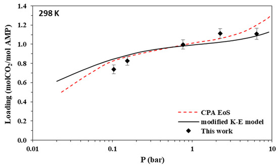
Figure 3.
Solubility of CO2 in aqueous AMP (17.7% wt.) solutions at 298 K. Experimental data (points, from this work) and correlations (lines) with the CPA equation of state and the modified Kent-Eisenberg model.
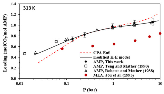
Figure 4.
Solubility of CO2 in aqueous AMP (17.7% wt.) solutions at 313 K (Data for MEA are also shown for comparison). Experimental data for AMP (points, from this work, Teng and Mather [30], and Roberts and Mather [28]), experimental data for MEA (solid circles, from Jou et al. [55]), and correlations (lines) with the CPA equation of state and the modified Kent-Eisenberg model.
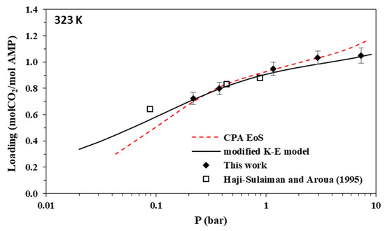
Figure 5.
Solubility of CO2 in aqueous AMP (17.7% wt.) solutions at 323 K. Experimental data (points, from this work and Hadji-Sulaiman and Aroua [32]) and correlations (lines) with the CPA equation of state and the modified Kent-Eisenberg model.
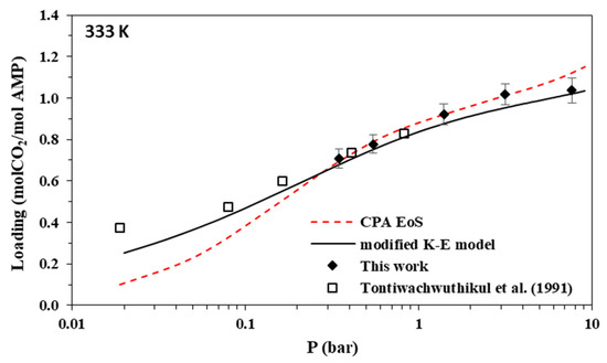
Figure 6.
Solubility of CO2 in aqueous AMP (17.7% wt.) solutions at 333 K. Experimental data (points, from this work and Tontiwachwuthikul et al. [31]) and correlations (lines) with the CPA equation of state and the modified Kent-Eisenberg model.
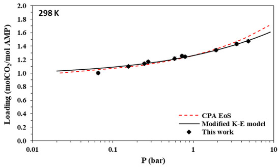
Figure 7.
Solubility of CO2 in aqueous MAPA (30.0% wt.) solutions at 298 K. Experimental data (points, from this work) and correlations (lines) with the CPA equation of state and the modified Kent-Eisenberg model.
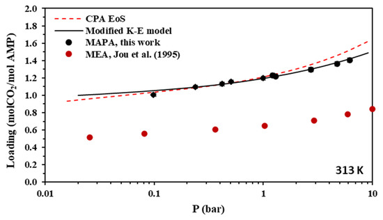
Figure 8.
Solubility of CO2 in aqueous MAPA (30.0% wt.) solutions at 313 K. Experimental data (points, from this work) and correlations (lines) with the CPA equation of state and the modified Kent-Eisenberg model. Experimental data for MEA [55] are also shown for comparison.
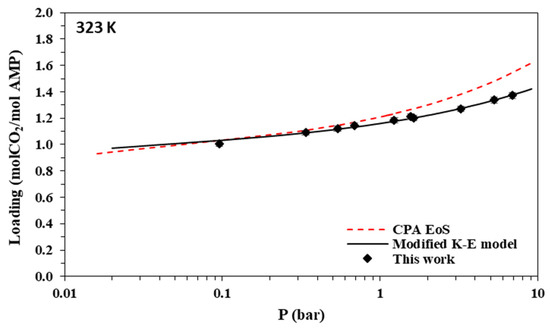
Figure 9.
Solubility of CO2 in aqueous MAPA (30.0% wt.) solutions at 323 K. Experimental data (points, from this work) and correlations (lines) with the CPA equation of state and the modified Kent-Eisenberg model.
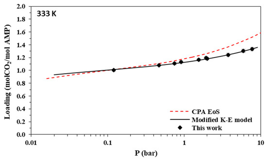
Figure 10.
Solubility of CO2 in aqueous MAPA (30.0% wt.) solutions at 333 K. Experimental data (points, from this work) and correlations (lines) with the CPA equation of state and the modified Kent-Eisenberg model.
As shown in Figure 4, the CO2 loading of the aqueous AMP solutions at 313 K and 0.1 bar, which are the usual conditions of the absorber in the relevant process, is approximately 0.7 mole of CO2 per mole of amine and reaches a value slightly above 1 mole of CO2 per mole of amine at higher CO2 partial pressures. Thus, the obtained experimental data confirm that AMP is performing as a sterically hindered amine, which presents a chemical absorption stoichiometric limit of 1 mole of per mole of amine. However, higher loadings are observed at higher pressures mainly due to physical absorption [14,23]. In addition, as shown in Figure 8, the CO2 loading of the aqueous MAPA solutions at 313 K and 0.1 bar, is approximately 1 mole of CO2 per mole of amine. Such loading values are expected, as MAPA molecules consist of two amine groups, one primary and one secondary, each of them presenting a chemical absorption stoichiometric limit of 0.5 moles of CO2 per mole of amine (group) [8,14,23].
4.2. CPA Modeling Results
As in our previous studies [23,24], the CPA was coupled with the pseudo-chemical reaction approach, i.e., to account for the CO2–amine chemical interactions as very strong specific interactions. This approximation is often used in equation of state models arising from their inability to explicitly account for chemical interactions [21,22].
Consequently, amine groups, primary and secondary, are modeled assuming that they have one proton donor and one proton acceptor site, which are able to form hydrogen bonds, and one chemical site that can only interact with CO2. Furthermore, CO2 is modeled assuming that it has one negative association site that can only interact with water and two (in cases of unhindered primary and secondary amines), or one (in cases of sterically hindered amines) chemical sites that can only associate with the relevant chemical site of the amine groups. In this way, as illustrated in Figure 11, the chemical absorption limit, presented in the Section 1, of 0.5 moles of CO2 per mole of unhindered primary or secondary amine and of 1 mole of CO2 per mole of hindered amine is preserved.
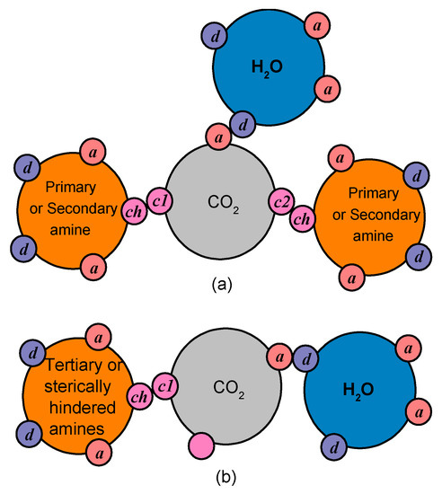
Figure 11.
The pseudo-chemical interactions for unhindered primary or secondary amines (a) and sterically hindered amines (b). The association sites are presented, i.e., sites for chemical interactions (ch, c1, c2), as well as proton donor (d) and proton acceptor sites (a) capable of hydrogen bonding.
The CPA pure fluid parameters for water and CO2 were adopted from Tsivintzelis et al. [61], whereas the amine parameters were estimated in this study. The AMP molecule, which presents one amine group and one hydroxyl, and the MAPA molecule, which presents two amine groups, one primary and one secondary, were modeled assuming four (equivalent for simplicity) association sites. Thus, the 4C association scheme was used in both cases. Their CPA pure fluid parameters were estimated by adjusting model predictions to available experimental data and/or to DIPRR correlations.
In more detail, the AMP parameters were estimated using the vapor pressure experimental data of Klepacova et al. [62], Barreau et al. [63], Belabbaci et al. [64], and Pappa et al. [65] and the liquid density data from Li and Lie [66]. The MAPA pure fluid parameters were estimated using the vapor pressure data of Kim et al. [67] and the experimental densities of Pinto et al. [68]. All pure fluid parameters used in this study are presented in Table 8. In all cases, model correlations present low absolute average deviations (AAD) for the used data, i.e., 0.14% and 1.53% for the AMP vapor pressures and molar volumes, respectively, and 1.52% and 0.37% for MAPA vapor pressures and molar volumes, respectively. The obtained CPA correlations are illustrated in Figures S1–S4 of the supplementary information file.
Table 8.
Pure fluid parameters used in this study.
The used binary parameters are presented in Table 9. Such parameters for the CO2–water sub-binary system were adopted form Tsivintzelis et al. [61], who suggested modeling CO2–water interactions assuming one association site on CO2 molecule, which is able to cross associate with water, while using the experimental value for the cross association energy. The binary interaction parameter, kij, for the AMP–water sub-binary system was estimated using the vapor–liquid equilibrium (VLE) experimental data of Pappa et al. [65]. It was found that, when using the CR-1 combining rule for the cross association interactions, the model satisfactorily describes the VLE of this system as shown in Figure S5 of the supplementary information file. For MAPA–water sub-binary systems, the experimental data of Kim et al. [67] for 373 K were used, and representative calculations are illustrated in Figure S6 of the supplementary information file.
Table 9.
CPA binary parameters used in this study.
Finally, the parameters for CO2–amine sub-binary systems were estimated by adjusting model predictions to the experimental data of this study. In all cases, a temperature independent kij was used. Considering the CO2–AMP system, it was found that the cross association energy of 318.9 bar∙L∙mol−1, reported for CO2–DETA and CO2–TETA systems in a previous study [24], gives rather satisfactory results and was also adopted for this system. For the same reason, the cross association energies used for CO2–MPA by Leontiadis et al. [23] were also adopted for the CO2–MAPA interactions. Such results indicate that, probably, universal parameters for the CO2–amine interactions can be estimated within the CPA model. Thus, in both cases only the cross association volumes were adjusted to the experimental data. All CPA calculations are presented in Figure 3, Figure 4, Figure 5, Figure 6, Figure 7, Figure 8, Figure 9 and Figure 10 and shown in Table 10 and Table 11; the percentage AADs of CPA correlations from the experimental data are 20.2 and 24.3% for AMP and MAPA solutions, respectively. Such rather high deviations are mainly observed due to the severe pseudo-chemical association approach, which, however, is necessary in such EoS models.
Table 10.
Percentage average absolute deviations (AAD %) of models’ correlations form the experimental data of this study for the CO2 loading of AMP solutions.
Table 11.
Percentage average absolute deviations (AAD %) of models’ correlations form the experimental data of this study for the CO2 loading of MAPA solutions.
It is worth noting that using the CPA model, seven adjustable parameters were used for modeling the solubility of CO2 in aqueous MEA solutions and five parameters for aqueous MDEA solutions by Wang et al. [25], whereas Leontiadis et al. [23] used six parameters for CO2–MPA and four binary parameters for CO2–MDEA pseudo-chemical interactions. Finally, Tzirakis et al. [24] used four adjustable parameters for CO2–DETA and CO2–TETA interactions. The rather high number of the parameters that need to be adjusted and the rather high value of the obtained kijs mainly occur due to the severe approximation of the pseudo-chemical reaction approach.
4.3. Kent-Eisenberg Model Results
As noted in the Section 1, AMP is sterically hindered and, thus, it is considered as a non-carbamate forming amine. Consequently, reaction (18) is not accounted for and Equations (34)–(36) are used to apply the Kent-Eisenberg model. On the other hand, MAPA is a diamine, consisting of a primary and a secondary amine group. In order to minimize the need for adjustable parameters, MAPA was modeled assuming equal and independent reactivity for each amine group, i.e., that the reactivity of each group does not depend on the potential reaction of the other one. This approximation was also used by Tzirakis et al. [70] to model the CO2 solubility in aqueous solutions of diamines. It resembles the Flory’s principle of independent reactivity, according to which the reactivity of each group is independent of the polymer chain length and is considered as a very good approximation for molecules (oligomers) with higher than 3–5 carbon atoms. Thus, MAPA was modeled using Equations (31)–(33). However, using the aforementioned approximation, all amine species concentrations shown in Equations (17)–(33) will denote moles of amine groups and not moles of molecules. In addition, the calculated loading from Equation (32) will denote the moles of absorbed CO2 per mole of amine groups (not molecules) and should be multiplied by two to be compared with the experimental results (which show moles of CO2 per mole of amine molecules).
In this work, we have decided to use the literature values of the parameters of Equation (36) for through and . Consequently, only the parameters of Equation (36) for and were adjusted to the experimental data of this work and to literature data (presented in Tables S1 and S2 of the supplementary information file, for AMP and MAPA solutions, respectively). All the available literature data points within the temperature range of 313 to 383 K and pressure range of 0.1 to 10 bar, plus the data of this work were included and equally weighted in the objective function. All the used parameters, obtained from literature or regressed in this work, for AMP and MAPA solutions are listed in Table 12.
Table 12.
Parameters of Equation (36) for AMP and MAPA aqueous solutions.
Using the parameters of Table 12, model-predicted CO2 loadings were compared to the experimental data of this work. The results for 2 M AMP and 3.35 M MAPA aqueous solutions are illustrated in Figure 3, Figure 4, Figure 5, Figure 6, Figure 7, Figure 8, Figure 9 and Figure 10 and, as parity plots, in Figures S7 and S8 of the supplementary information file. The obtained deviations of model correlations from the experimental data of this work are shown in Table 10 and Table 11, for AMP and MAPA solutions, respectively. In more detail, using two parameters adjusted to the experimental data (A and D parameters of Table 12 for K1 AMP), the model presents an overall percentage average deviation from the experimental data of this study equal to 3.7%. Using two additional adjustable parameters for MAPA (A and D parameters of Table 12 for K1 MAPA and K2 MAPA), the observed deviations are significantly lower and equal to 1%. Such rather low deviations reveal that the model, although very approximate, allows the correct description of the experimental data if appropriate values of the adjustable parameters are selected, i.e., effective values that, according to Jou et al. [52], absorb all non-idealities of the system. Compared to the CPA EoS, it presents significantly more accurate correlations, however, using more adjustable parameters.
Because the modified Kent-Eisenberg model resulted in more accurate correlations, it was subsequently used to predict the speciation of the loaded liquid phase for both amine systems. Results for 313 K are presented in Figure 12 and Figure 13, whereas the other investigated temperatures are shown in Figures S9–S14 of the supplementary information file. It is observed that the free amine concentration becomes very low at CO2 partial pressures higher than approximately 1 bar, whereas at higher CO2 partial pressures, the increase of the overall CO2 solubility mainly proceeds through the molecular CO2 dissolution, as shown by the respective molecular CO2 curve of Figure 12 and Figure 13, and the carbamate hydrolysis, in the case of MAPA, as shown by the RRNCOO− curve in Figure 13.
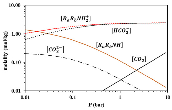
Figure 12.
Liquid-phase speciation for AMP-CO2-H2O system at 313 K, predicted using the modified Kent-Eisenberg model (calculations performed for the CO2 loading of 17.7% wt. AMP aqueous solutions).
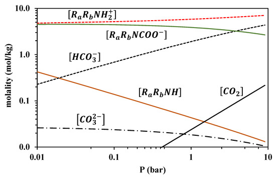
Figure 13.
Liquid-phase speciation for MAPA-CO2-H2O system at 313 K, predicted using modified the Kent-Eisenberg model (calculations performed for the CO2 loading of 30.0% wt. MAPA aqueous solutions).
5. Conclusions
In this study, the solubility of CO2 in 17.7% wt. (approximately 2M) aqueous 2-amino-2-methyl-1-propanol (AMP) and 30.0% wt. (approximately 3.36 M) 3-(methylamino)propylamine (MAPA) solutions was experimentally measured, in the 298–333 K temperature range, using a pressure decay method. Because the available literature experimental data for MAPA aqueous solutions are very limited, the experimental results of this study were compared to respective literature data only for AMP aqueous systems, and a rather satisfactory agreement was observed. Such experimental data are useful in parameterizing thermodynamic models. Consequently, they were used to parameterize the CPA equation of state coupled with the pseudo-chemical reaction approach, which is a severe, but necessary, approximation in order to apply such thermodynamic models, and the modified Kent-Eisenberg model, which is an approximate semi-empirical model. It is observed that the modified Kent-Eisenberg model correlations present a very satisfactory agreement with the experimental data. Compared to the CPA EoS, the Kent-Eisenberg model presents significantly more accurate correlations, but at the cost of more adjustable parameters. Considering also its low complexity compared to association models, it could be a rather satisfactory choice if, other than the CO2 solubility, no other thermodynamic properties are needed. However, if other properties, such as densities of phases in equilibrium or thermal properties, are needed in engineering design applications, the choice of a thermodynamic model, such as an equation of state model, is mandatory.
Supplementary Materials
The following supporting information can be downloaded at: https://www.mdpi.com/article/10.3390/separations9110338/s1, Figure S1: Vapor pressure of AMP. Experimental data (points, [54,62,63,64,65]) and CPA correlations (lines); Figure S2: Molar volume of AMP. Experimental data (points, [54,66]) and CPA correlations (lines); Figure S3: Vapor pressures of MAPA. Experimental data (points, [67]) and CPA correlations (lines); Figure S4: Molar volume of MAPA. Experimental data (points, [68]) and CPA correlations (lines); Figure S5: AMP–water VLE. Experimental data from Pappa et al. [65] (points) and CPA correlations (lines); Figure S6: MAPA–water VLE. Experimental data from Kim et al. [67] (points) and CPA correlations (lines); Figure S7: Parity plot of calculated (with the Kent-Eisenberg model) against experimental (this work) loadings of aqueous AMP solutions; Figure S8: Parity plot of calculated (with the Kent-Eisenberg model) against experimental (this work) loadings of aqueous MAPA solutions; Figure S9: Liquid-phase speciation for AMP-CO2-H2O system at 298 K, calculated using the modified Kent-Eisenberg model; Figure S10: Liquid-phase speciation for AMP-CO2-H2O system at 323 K, calculated using the modified Kent-Eisenberg model; Figure S11: Liquid-phase speciation for AMP-CO2-H2O system at 333 K, calculated using the modified Kent-Eisenberg model; Figure S12: Liquid-phase speciation for MAPA-CO2-H2O system at 298 K, calculated using the modified Kent-Eisenberg model; Figure S13: Liquid-phase speciation for MAPA-CO2-H2O system at 323 K, calculated using the modified Kent-Eisenberg model; Figure S14: Liquid-phase speciation for MAPA-CO2-H2O system at 333 K, calculated using the modified Kent-Eisenberg model; Table S1: Summary of literature sources of experimental solubility data used for adjusting the parameters A and D (Equation (36)) for AMP-CO2-H2O system; Table S2: Summary of literature sources of experimental solubility data used for adjusting the parameters A and D (Equation (36)) for MAPA-CO2-H2O system.
Author Contributions
Conceptualization, I.T. and G.K.; methodology, I.T., E.T. and G.K.; software, I.T. and G.K.; validation, I.T. and G.K.; formal analysis, I.T. and G.K.; investigation, G.K. and M.A.S.; resources, I.T. and E.T.; data curation, I.T., M.A.S. and G.K.; writing—original draft preparation, I.T. and G.K.; writing—review and editing, I.T. and G.K.; visualization, I.T. and G.K.; supervision, I.T.; funding acquisition, G.K. All authors have read and agreed to the published version of the manuscript.
Funding
This work was co-financed by Greece and the EU through the Operational Program “Human Resources Development through PhD studies”, implemented by State Scholarships Foundation (IKY).
Data Availability Statement
All data are reported in the article.
Acknowledgments
G.K. would like to acknowledge State Scholarships Foundation (IKY) of Greece, as this work was co-financed by Greece and the EU through the Operational Program “Human Resources Development through PhD studies”, implemented by State Scholarships Foundation (IKY).
Conflicts of Interest
The authors declare no conflict of interest.
References
- Cannone, S.F.; Lanzini, A.; Santarelli, M. A review on CO2 capture technologies with focus on CO2-enhanced methane recovery from hydrates. Energies 2021, 14, 387. [Google Scholar] [CrossRef]
- Koukouzas, N.; Christopoulou, M.; Giannakopoulou, P.P.; Rogkala, A.; Gianni, E.; Karkalis, C.; Pyrgaki, K.; Krassakis, P.; Koutsovitis, P.; Panagiotaras, D.; et al. Current CO2 capture and storage trends in Europe in a view of social knowledge and acceptance. A short review. Energies 2022, 15, 5716. [Google Scholar] [CrossRef]
- WRI. Climate Analysis Indicators Tool; World Resources Institute: Washington, DC, USA, 2007. [Google Scholar]
- Ritchie, H.; Roser, M.; Rosado, P. CO2 and Greenhouse Gas Emissions. 2020. Available online: https://ourworldindata.org/co2-and-other-greenhouse-gas-emissions (accessed on 20 December 2020).
- Kenarsari, S.D.; Yang, D.; Jiang, G.; Zhang, S.; Wang, J.; Russell, A.G.; Wei, Q.; Fan, M. Review of recent advances in carbon dioxide separation and capture. RSC Adv. 2013, 3, 22739–22773. [Google Scholar] [CrossRef]
- Rochelle, G.T. Amine scrubbing for CO2 capture. Science 2009, 325, 1652–1654. [Google Scholar] [CrossRef]
- Bui, M.; Adjiman, C.S.; Bardow, A.; Anthony, E.J.; Boston, A.; Brown, S.; Fennell, P.S.; Fuss, S.; Galindo, A.; Hackett, L.A.; et al. Carbon capture and storage (CCS): The way forward. Energy Environ. Sci. 2018, 11, 1062–1176. [Google Scholar] [CrossRef]
- Papadopoulos, A.I.; Tzirakis, F.; Tsivintzelis, I.; Seferlis, P. Phase-change solvents and processes for postcombustion CO2 capture: A detailed review. Ind. Eng. Chem. Res. 2019, 58, 5088–5111. [Google Scholar] [CrossRef]
- Papadopoulos, A.I.; Perdomo, F.A.; Tzirakis, F.; Shavalieva, G.; Tsivintzelis, I.; Kazepidis, P.; Nessi, E.; Papadokonstantakis, S.; Seferlis, P.; Galindo, A.; et al. Molecular engineering of sustainable phase-change solvents: From digital design to scaling-up for CO2 capture. Chem. Eng. J. 2021, 420, 127624. [Google Scholar] [CrossRef]
- Arshad, M.W.; Svendsen, H.F.; Fosbøl, P.L.; von Solms, N.; Thomsen, K. Equilibrium total pressure and CO2 solubility in binary and ternary aqueous solutions of 2-(diethylamino) ethanol (DEEA) and 3-(methylamino) propylamine (MAPA). J. Chem. Eng. Data 2014, 59, 764–774. [Google Scholar] [CrossRef]
- Caplow, M. Kinetics of carbamate formation and breakdown. J. Am. Chem. Soc. 1968, 90, 6795–6803. [Google Scholar] [CrossRef]
- Danckwerts, P.V. The reaction of CO2 with ethanolamines. Chem. Eng. Sci. 1979, 34, 443–446. [Google Scholar] [CrossRef]
- Sartori, G.; Savage, D.W. Sterically hindered amines for carbon dioxide removal from gases. Ind. Eng. Chem. Fundam. 1983, 22, 239–249. [Google Scholar] [CrossRef]
- Zhang, J. Study on CO2 Capture Using Thermomorphic Biphasic Solvents with Energy Efficient Regeneration. Ph.D. Thesis, Dortmund Technische Universität, Dortmund, Germany, 2014. [Google Scholar]
- Tzirakis, F.; Tsivintzelis, I.; Papadopoulos, A.I.; Seferlis, P. Experimental measurement and assessment of equilibrium behaviour for phase change solvents used in CO2 capture. Chem. Eng. Sci. 2019, 199, 20–27. [Google Scholar] [CrossRef]
- Tzirakis, F.; Tsivintzelis, I.; Papadopoulos, A.I.; Seferlis, P. Experimental investigation of phase change amine solutions used in CO2 capture applications: Systems with dimethylcyclohexylamine (DMCA) and N-cyclohexyl-1,3-propanediamine (CHAP) or 3-methylaminopropylamine (MAPA). Int. J. Greenh. Gas Control. 2021, 109, 103353. [Google Scholar] [CrossRef]
- Pinto, D.D.; Zaidy, S.A.; Hartono, A.; Svendsen, H.F. Evaluation of a phase change solvent for CO2 capture: Absorption and desorption tests. Int. J. Greenh. Gas Control. 2014, 28, 318–327. [Google Scholar] [CrossRef]
- Uyan, M.; Sieder, G.; Ingram, T.; Held, C. Predicting CO2 solubility in aqueous N-methyldiethanolamine solutions with ePC-SAFT. Fluid Phase Equilib. 2015, 393, 91–100. [Google Scholar] [CrossRef]
- Wangler, A.; Sieder, G.; Ingram, T.; Heilig, M.; Held, C. Prediction of CO2 and H2S solubility and enthalpy of absorption in reacting N-methyldiethanolamine/water systems with ePC-SAFT. Fluid Phase Equilib. 2018, 461, 15–27. [Google Scholar] [CrossRef]
- Suleman, H.; Maulud, A.S.; Man, Z. Review and selection criteria of classical thermodynamic models for acid gas absorption in aqueous alkanolamines. Rev. Chem. Eng. 2015, 31, 599–639. [Google Scholar] [CrossRef]
- Rodriguez, J.; Mac Dowell, N.; Llovell, F.; Adjiman, C.S.; Jackson, G.; Galindo, A. Modelling the fluid phase behaviour of aqueous mixtures of multifunctional alkanolamines and carbon dioxide using transferable parameters with the SAFT-VR approach. Mol. Phys. 2012, 110, 1325–1348. [Google Scholar] [CrossRef]
- Chremos, A.; Forte, E.; Papaioannou, V.; Galindo, A.; Jackson, G.; Adjiman, C.S. Modelling the phase and chemical equilibria of aqueous solutions of alkanolamines and carbon dioxide using the SAFT-γ SW group contribution approach. Fluid Phase Equilib. 2016, 407, 280–297. [Google Scholar] [CrossRef]
- Leontiadis, K.; Tzimpilis, E.; Aslanidou, D.; Tsivintzelis, I. Solubility of CO2 in 3-amino-1-propanol and in N-methyldiethanolamine aqueous solutions: Experimental investigation and correlation using the CPA equation of state. Fluid Phase Equilib. 2019, 500, 112254. [Google Scholar] [CrossRef]
- Tzirakis, F.; Papadopoulos, A.I.; Seferlis, P.; Tsivintzelis, I. CO2 Solubility in diethylenetriamine (DETA) and triethylenetetramine (TETA) aqueous mixtures: Experimental investigation and correlation using the CPA equation of state. Chem. Thermodyn. Therm. Anal. 2021, 3, 100017. [Google Scholar] [CrossRef]
- Wang, T.; El Ahmar, E.; Coquelet, C.; Kontogeorgis, G.M. Improvement of the PR-CPA equation of state for modelling of acid gases solubilities in aqueous alkanolamine solutions. Fluid Phase Equilib. 2018, 471, 74–87. [Google Scholar] [CrossRef]
- Chen, X.; Closmann, F.; Rochelle, G.T. Accurate screening of amines by the wetted wall column. Energy Procedia 2011, 4, 101–108. [Google Scholar] [CrossRef]
- Voice, A.K.; Vevelstad, S.J.; Chen, X.; Nguyen, T.; Rochelle, G.T. Aqueous 3-(methylamino) propylamine for CO2 capture. Int. J. Greenh. Gas Control. 2013, 15, 70–77. [Google Scholar] [CrossRef]
- Roberts, B.E.; Mather, A.E. Solubility of CO2 and H2S in a hindered amine solution. Chem. Eng. Comm. 1988, 64, 105–111. [Google Scholar] [CrossRef]
- Teng, T.T.; Mather, A.E. Solubility of H2S, CO2 and their mixtures in an AMP solution. Can. J. Chem. Eng. 1989, 67, 846–850. [Google Scholar] [CrossRef]
- Teng, T.T.; Mather, A.E. Solubitiy of CO2 in an AMP solution. J. Chem. Eng. Data 1990, 35, 410–411. [Google Scholar] [CrossRef]
- Tontiwachwuthikul, P.; Meisen, A.; Lim, C.J. Solubility of CO2 in 2-Amino-2-methyl-1-propanol Solutions. J. Chem. Eng. Data 1991, 36, 130–133. [Google Scholar] [CrossRef]
- Haji-Sulaiman, M.Z.; Aroua, M.K. Equilibrium of CO2 in aqueous diethanolamine (DEA) and amino methyl propanol (AMP) solutions. Chem. Eng. Comm. 1995, 140, 157–171. [Google Scholar] [CrossRef]
- Haji-Sulaiman, M.Z.; Aroua, M.K.; Pervez, M.I. Equilibrium concentration profiles of species in CO2—Alkanolamine—Water systems. Gas Sep. Purif. 1996, 10, 13–18. [Google Scholar] [CrossRef]
- Jane, I.S.; Li, M.H. Solubilities of mixtures of carbon dioxide and hydrogen sulfide in water + diethanolamine + 2-amino-2-methyl-1-propanol. J. Chem. Eng. Data 1997, 42, 98–105. [Google Scholar] [CrossRef]
- Silkenbäumer, D.; Rumpf, B.; Lichtenthaler, R.N. Solubility of carbon dioxide in aqueous solutions of 2-Amino-2-methyl-1-propanol and N-Methyldiethanolamine and their mixtures in the temperature range from 313 to 353 K and pressures up to 2.7 MPa. Ind. Eng. Chem. Res. 1998, 37, 3133–3141. [Google Scholar] [CrossRef]
- Park, S.H.; Lee, K.B.; Hyun, J.C.; Kim, S.H. Correlation and prediction of the solubility of carbon dioxide in aqueous alkanolamine and mixed alkanolamine solutions. Ind. Eng. Chem. Res. 2002, 41, 1658–1665. [Google Scholar] [CrossRef]
- Kundu, M.; Mandal, B.P.; Bandyopadhyay, S.S. Vapor—Liquid equilibrium of CO2 in aqueous solutions of 2-Amino-2-methyl-1-propanol. J. Chem. Eng. Data 2003, 48, 789–796. [Google Scholar] [CrossRef]
- Tobiesen, F.A.; Svendsen, H.F.; Mejdell, T. Modeling of blast furnace CO2 capture using amine absorbents. Ind. Eng. Chem. Res. 2007, 46, 7811–7819. [Google Scholar] [CrossRef]
- Arcis, H.; Rodier, L.; Coxam, J.Y. Enthalpy of solution of CO2 in aqueous solutions of 2-amino-2-methyl-1-propanol. J. Chem. Thermodyn. 2007, 39, 878–887. [Google Scholar] [CrossRef]
- Yang, Z.Y.; Soriano, A.N.; Caparanga, A.R.; Li, M.H. Equilibrium solubility of carbon dioxide in (2-amino-2-methyl-1-propanol + piperazine + water). J. Chem. Thermodyn. 2010, 42, 659–665. [Google Scholar] [CrossRef]
- Dash, S.K.; Samanta, A.N.; Bandyopadhyay, S.S. (Vapour + liquid) equilibria (VLE) of CO2 in aqueous solutions of 2-amino-2-methyl-1-propanol: New data and modelling using eNRTL-equation. J. Chem. Thermodyn. 2011, 43, 1278–1285. [Google Scholar] [CrossRef]
- Shariff, A.M.; Murshid, G.G.; Lau, K.K.; Bustam, M.A.; Ahmad, F. Solubility of CO2 in aqueous solutions of 2-amino-2-methyl-1-propanol at high pressure. Int. J. Environ. Ecol. Eng. 2011, 5, 825–828. [Google Scholar]
- Tong, D.; Trusler, J.M.; Maitland, G.C.; Gibbins, J.; Fennell, P.S. Solubility of carbon dioxide in aqueous solution of monoethanolamine or 2-amino-2-methyl-1-propanol: Experimental measurements and modelling. Int. J. Greenh. Gas Control. 2012, 6, 37–47. [Google Scholar] [CrossRef]
- Nordin, S.; Salleh, R.M.; Ismail, N. 2013 experimental study on CO2 absorption in aqueous mixtures of 2-amino-2-methyl-1-propanol and N-butyl-3-methylpyridinium tetrafluoroborate. In Proceedings of the IEEE Business Engineering and Industrial Applications Colloquium (BEIAC), Langkawi, Malaysia, 7–9 April 2013; pp. 549–552. [Google Scholar]
- Tong, D.; Maitland, G.C.; Trusler, M.J.; Fennell, P.S. Solubility of carbon dioxide in aqueous blends of 2-amino-2-methyl-1-propanol and piperazine. Chem. Eng. Sci. 2013, 101, 851–864. [Google Scholar] [CrossRef]
- Li, H.; Frailie, P.T.; Rochelle, G.T.; Chen, J. Thermodynamic modeling of piperazine/2-aminomethylpropanol/CO2/water. Chem. Eng. Sci. 2014, 117, 331–341. [Google Scholar] [CrossRef]
- Nouacer, A.; Belaribi, F.B.; Mokbel, I.; Jose, J. Solubility of carbon dioxide gas in some 2.5 M tertiary amine aqueous solutions. J. Mol. Liq. 2014, 190, 68–73. [Google Scholar] [CrossRef]
- Kortunov, P.V.; Siskin, M.; Paccagnini, M.; Thomann, H. CO2 reaction mechanisms with hindered alkanolamines: Control and promotion of reaction pathways. Energy Fuels 2016, 30, 1223–1236. [Google Scholar]
- Narku-Tetteh, J.; Muchan, P.; Saiwan, C.; Supap, T.; Idem, R. Selection of components for formulation of amine blends for post combustion CO2 capture based on the side chain structure of primary, secondary and tertiary amines. Chem. Eng. Sci. 2017, 170, 542–560. [Google Scholar] [CrossRef]
- Hartono, A.; Ahmad, R.; Usman, M.; Asif, N.; Svendsen, H.F. Solubility of CO2 in 0.1 M, 1 M and 3 M of 2-amino-2-methyl-1-propanol (AMP) from 313 to 393K and model representation using the eNRTL framework. Fluid Phase Equilib. 2020, 511, 112485. [Google Scholar] [CrossRef]
- Kent, R.L.; Eisenberg, B. Better data for amine treating. Hydrocarb. Process 1976, 55, 87–90. [Google Scholar]
- Jou, F.-Y.; Mather, A.E.; Otto, F.D. Solubility of H2S and CO2 in aqueous methyldiethanolamine solutions. Ind. Eng. Chem. Proc. Des. Dev. 1982, 21, 539–544. [Google Scholar] [CrossRef]
- Suleman, H.; Maulud, A.S.; Fosbøl, P.L.; Nasir, Q.; Nasir, R.; Shahid, M.Z.; Nawaz, M.; Abunowara, M. A review of semi-empirical equilibrium models for CO2-alkanolamine-H2O solutions and their mixtures at high pressure. J. Environ. Chem. Eng. 2021, 9, 104713. [Google Scholar] [CrossRef]
- National Institute of Standards and Technology (NIST). Isothermal Properties for Carbon Dioxide. Available online: https://webbook.nist.gov/chemistry/ (accessed on 31 May 2019).
- Jou, F.Y.; Mather, A.E.; Otto, F.D. The solubility of CO2 in a 30 mass percent monoethanolamine solution. Can. J. Chem. Eng. 1995, 73, 140–147. [Google Scholar] [CrossRef]
- Wertheim, M.S. Fluids with highly directional attractive forces. III. Multiple attraction sites. J. Stat. Phys. 1986, 42, 459–476. [Google Scholar] [CrossRef]
- Kontogeorgis, G.M.; Voutsas, E.C.; Yakoumis, I.V.; Tassios, D.P. An equation of state for associating fluids. Ind. Eng. Chem. Res. 1996, 35, 4310–4318. [Google Scholar] [CrossRef]
- Kontogeorgis, G.M.; Michelsen, M.L.; Folas, G.K.; Derawi, S.; Von Solms, N.; Stenby, E.H. Ten years with the CPA (Cubic-Plus-Association) equation of state. Part 2. Cross-associating and multicomponent systems. Ind. Eng. Chem. Res. 2006, 45, 4869–4878. [Google Scholar] [CrossRef]
- Tsivintzelis, I.; Kontogeorgis, G.M.; Michelsen, M.L.; Stenby, E.H. Modeling phase equilibria for acid gas mixtures using the CPA equation of state. I. Mixtures with H2S. AIChE J. 2010, 56, 2965–2982. [Google Scholar] [CrossRef]
- Haji-Sulaiman, M.Z.; Aroua, M.K.; Benamor, A. Analysis of equilibrium data of CO2 in aqueous solutions of diethanolamine (DEA), methyldiethanolamine (MDEA) and their mixtures using the modified Kent Eisenberg model. Chem. Eng. Res. Des. 1998, 76, 961–968. [Google Scholar] [CrossRef]
- Tsivintzelis, I.; Kontogeorgis, G.M.; Michelsen, M.L.; Stenby, E.H. Modeling phase equilibria for acid gas mixtures using the CPA equation of state. Part II: Binary mixtures with CO2. Fluid Phase Equilib. 2011, 306, 38–56. [Google Scholar] [CrossRef]
- Klepácová, K.; Huttenhuis, P.J.; Derks, P.W.; Versteeg, G.F. Vapor pressures of several commercially used alkanolamines. J. Chem. Eng. Data 2011, 56, 2242–2248. [Google Scholar] [CrossRef][Green Version]
- Barreau, A.; Mougin, P.; Lefebvre, C.; Luu Thi, Q.M.; Rieu, J. Ternary isobaric vapor—Liquid equilibria of methanol + N-methyldiethanolamine + water and methanol + 2-amino-2-methyl-1-propanol + water systems. J. Chem. Eng. Data 2007, 52, 769–773. [Google Scholar] [CrossRef]
- Belabbaci, A.; Ahmed, N.C.B.; Mokbel, I.; Negadi, L. Investigation of the isothermal (vapour + liquid) equilibria of aqueous 2-amino-2-methyl-1-propanol (AMP), N-benzylethanolamine, or 3-dimethylamino-1-propanol solutions at several temperatures. J. Chem. Thermodyn. 2010, 42, 1158–1162. [Google Scholar] [CrossRef]
- Pappa, G.D.; Anastasi, C.; Voutsas, E.C. Measurement and thermodynamic modeling of the phase equilibrium of aqueous 2-amino-2-methyl-1-propanol solutions. Fluid Phase Equilib. 2006, 243, 193–197. [Google Scholar] [CrossRef]
- Li, M.H.; Lie, Y.C. Densities and viscosities of solutions of monoethanolamine + N-methyldiethanolamine + water and monoethanolamine + 2-amino-2-methyl-1-propanol + water. J. Chem. Eng. Data 1994, 39, 444–447. [Google Scholar] [CrossRef]
- Kim, I.; Svendsen, H.F.; Børresen, E. Ebulliometric determination of vapor−liquid equilibria for pure water, monoethanolamine, n-methyldiethanolamine, 3-(methylamino)-propylamine, and their binary and ternary solutions. J. Chem. Eng. Data 2008, 53, 2521–2531. [Google Scholar] [CrossRef]
- Pinto, D.D.; Monteiro, J.G.S.; Johnsen, B.; Svendsen, H.F.; Knuutila, H. Density measurements and modelling of loaded and unloaded aqueous solutions of MDEA (N-methyldiethanolamine), DMEA (N,N-dimethylethanolamine), DEEA (diethylethanolamine) and MAPA (N-methyl-1,3-diaminopropane). Int. J. Greenh. Gas Control. 2014, 25, 173–185. [Google Scholar] [CrossRef]
- Constantinou, L.; Gani, R. New group contribution method for estimating properties of pure compounds. AIChE J. 1994, 40, 1697–1710. [Google Scholar] [CrossRef]
- Tzirakis, F.; Papadopoulos, A.I.; Seferlis, P.; Tsivintzelis, I. CO2 solubility in aqueous methylcyclohexylamine (MCA) and N-cyclohexyl-1,3-propanediamine (CHAP) solutions. AIChE J. 2022; submitted for publication. [Google Scholar]
- Edwards, T.J.; Maurer, G.; Newman, J.; Prausnitz, J.M. Vapor-liquid equilibria in multicomponent aqueous solutions of volatile weak electrolytes. AIChE J. 1978, 24, 966–976. [Google Scholar] [CrossRef]


Publisher’s Note: MDPI stays neutral with regard to jurisdictional claims in published maps and institutional affiliations. |
© 2022 by the authors. Licensee MDPI, Basel, Switzerland. This article is an open access article distributed under the terms and conditions of the Creative Commons Attribution (CC BY) license (https://creativecommons.org/licenses/by/4.0/).