
Modeling the Effects of Seasonal Weathering on Centrifuged Oil Sands Tailings


Abstract
:1. Introduction
2. Tailings Material and Characterization
3. Laboratory Setup
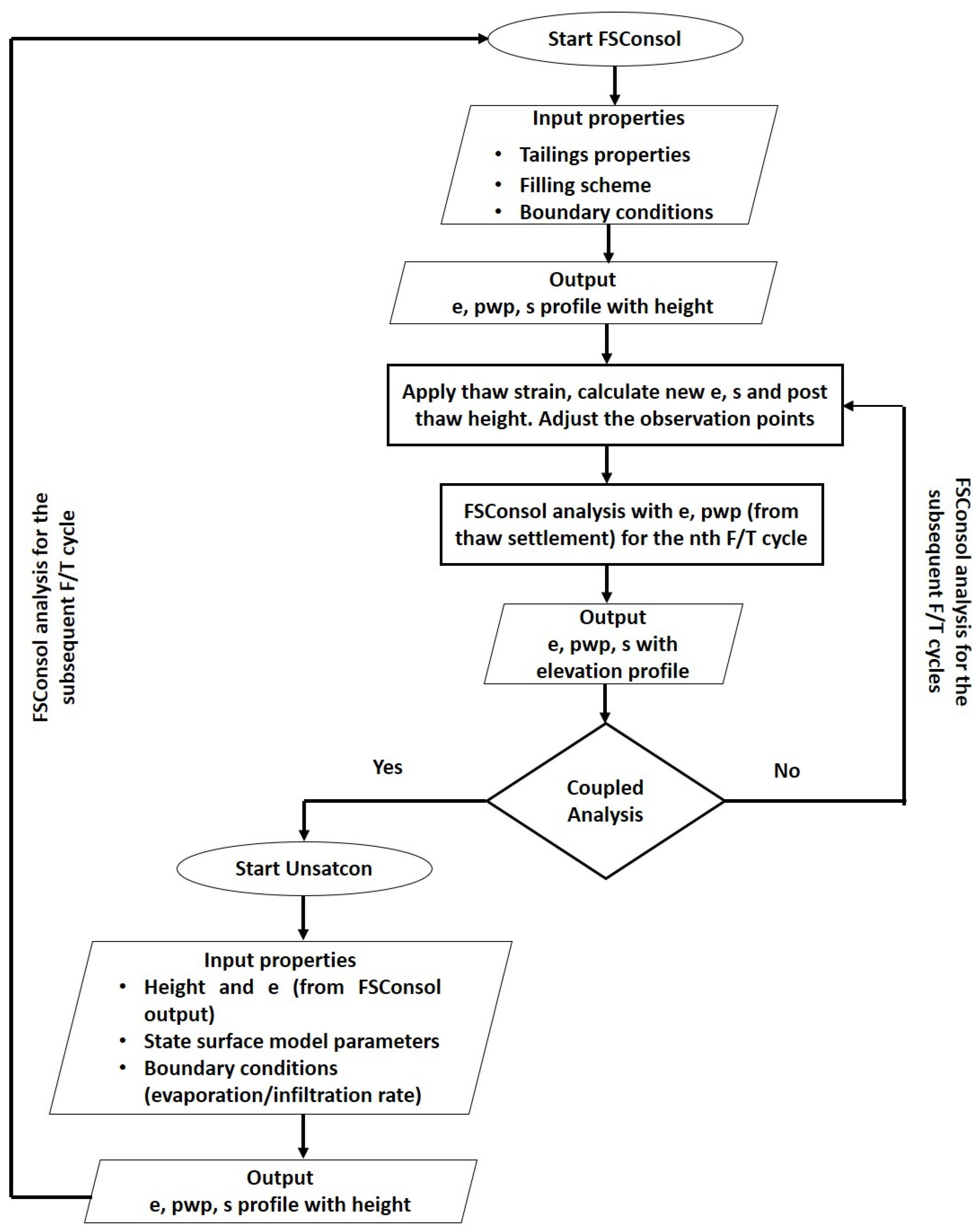
4. Coupled Modeling
4.1. Modeling Analysis Development
4.2. Numerical Model Parameters
5. Modeling Results
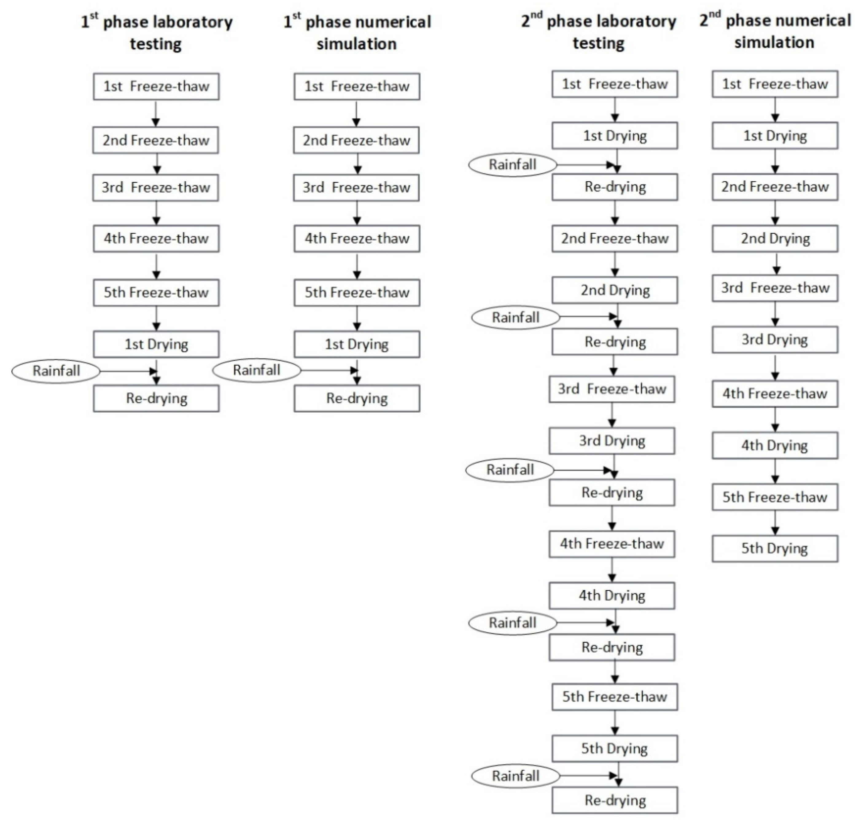
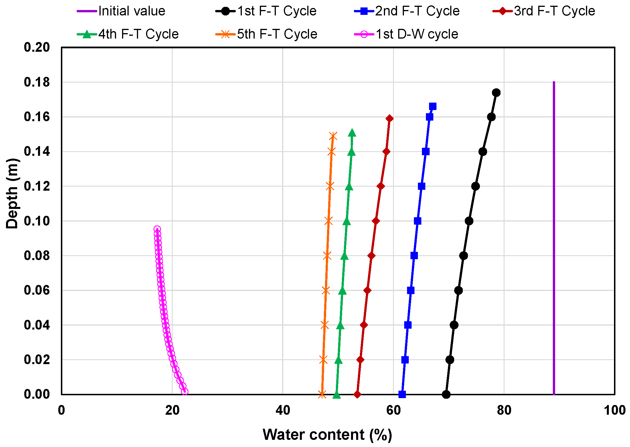
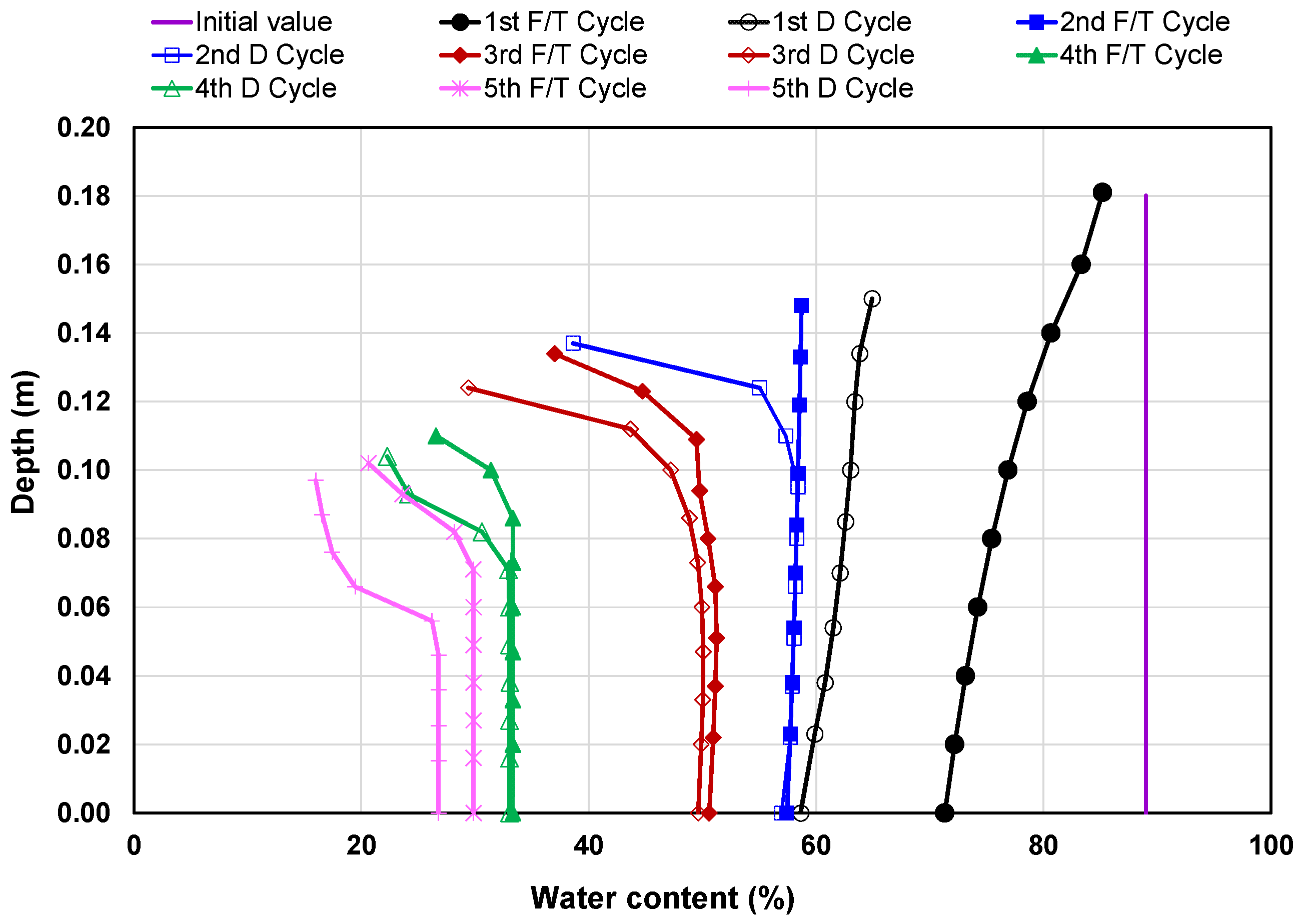
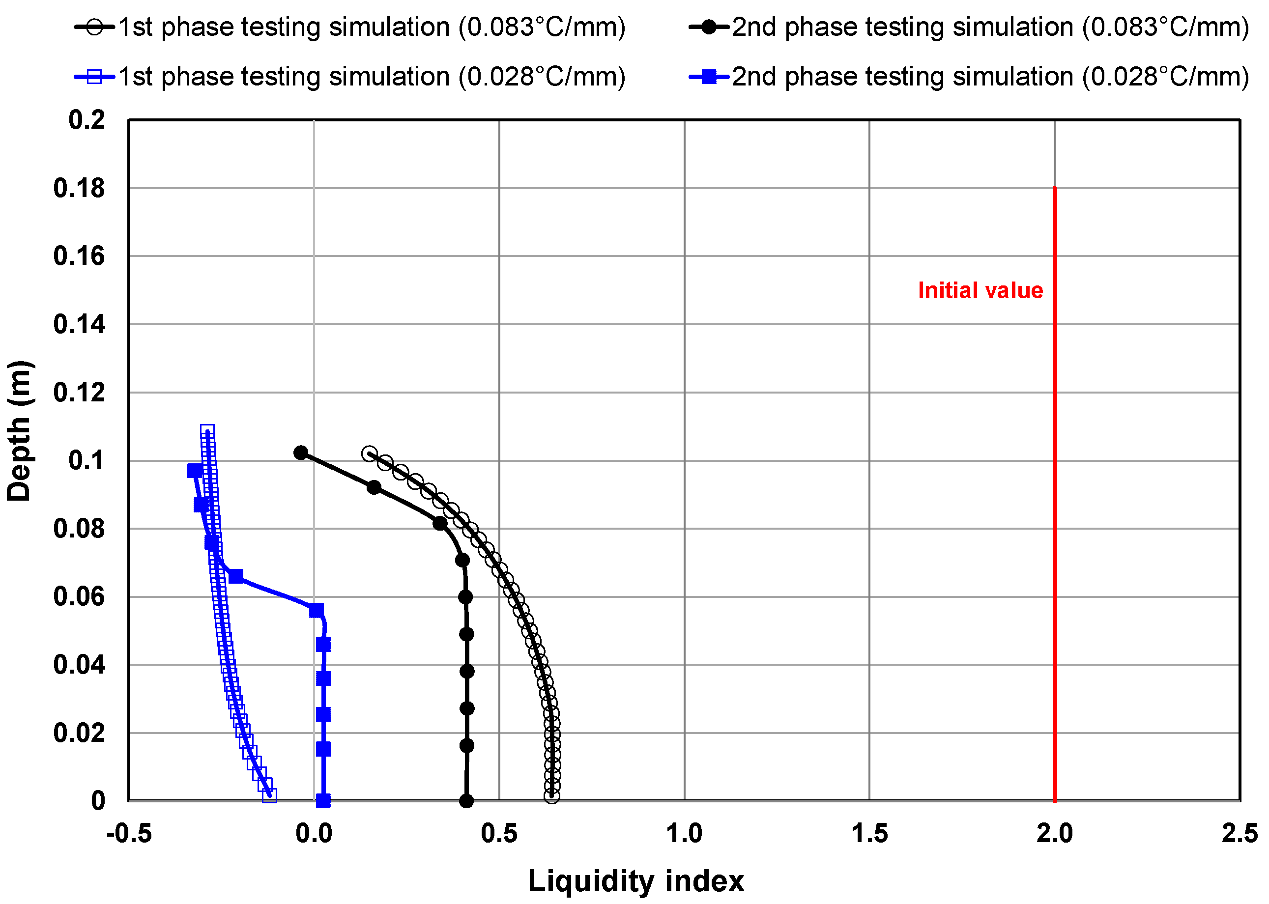
5.1. Numerical Simulation of First-Phase Testing
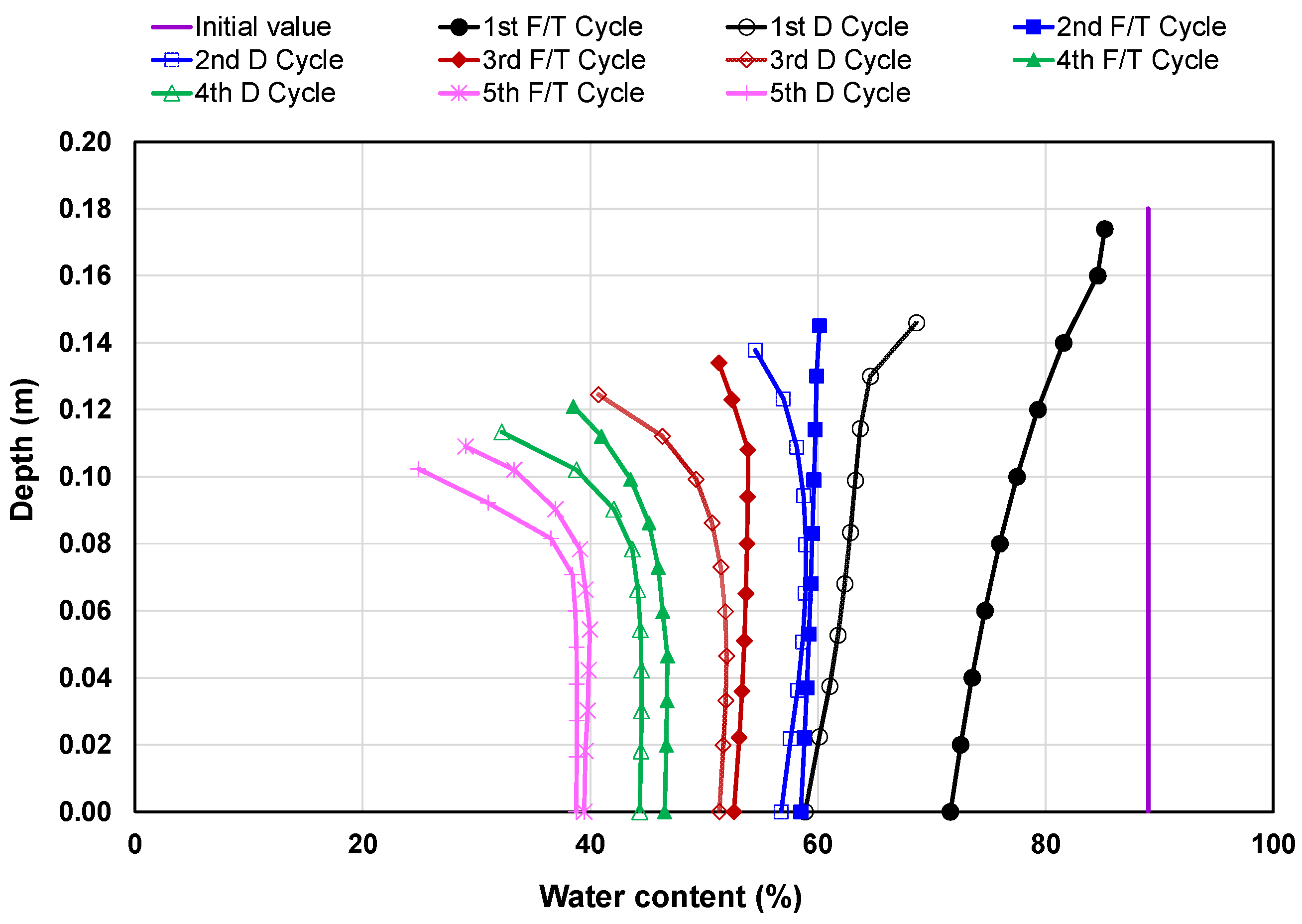
5.2. Numerical Simulation of Second-Phase Testing
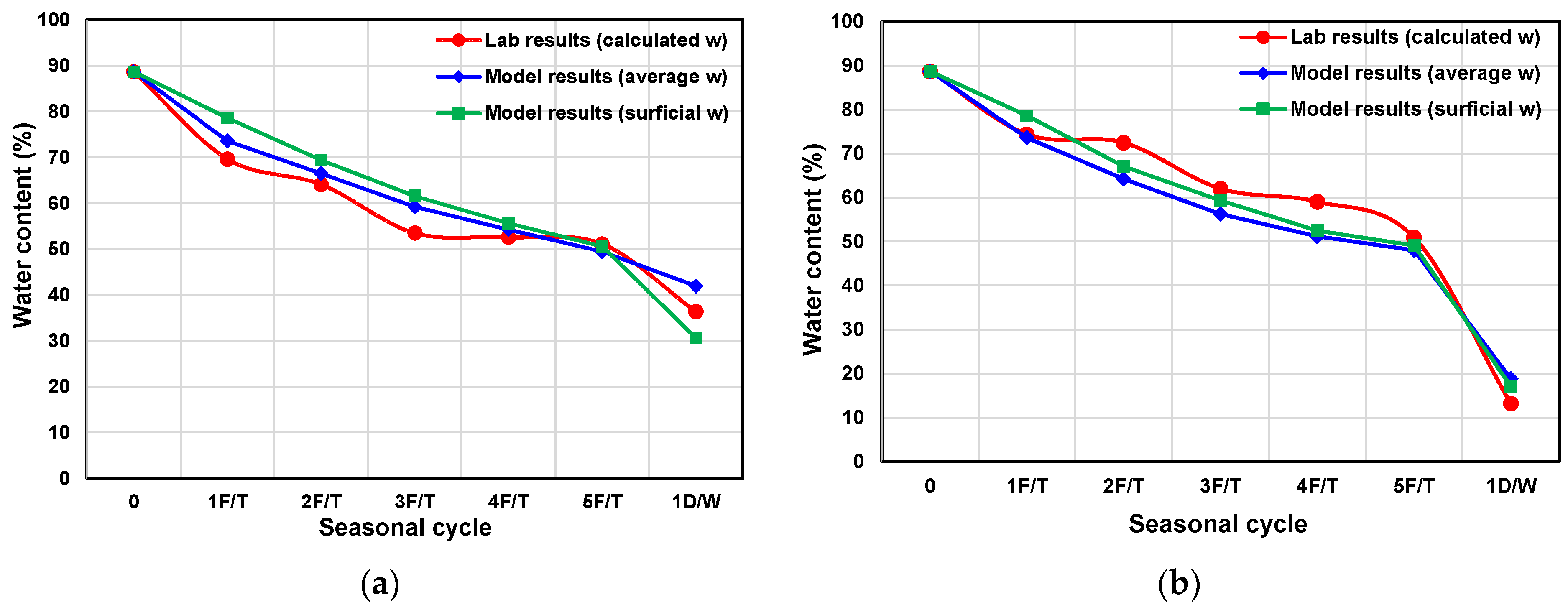
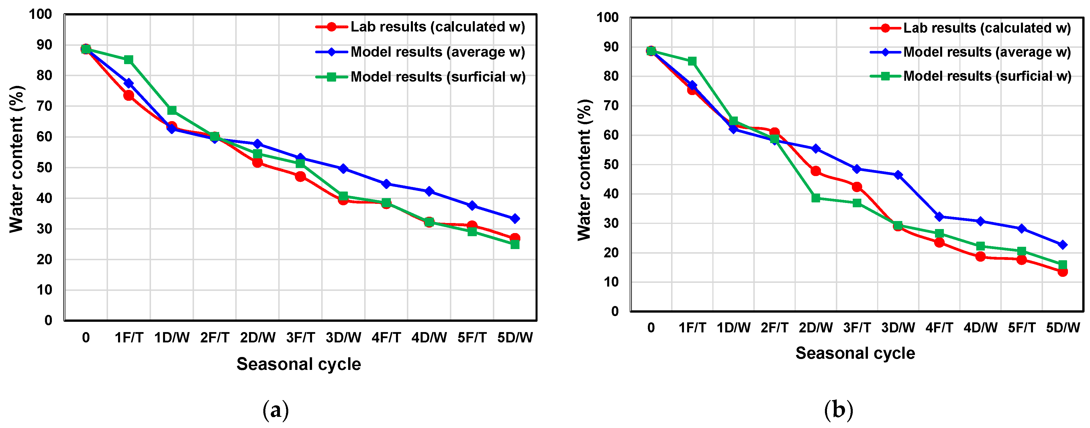
5.3. Comparison between the Model and Laboratory Results
6. Discussion
7. Conclusions
Author Contributions
Funding
Data Availability Statement
Acknowledgments
Conflicts of Interest
References
- Government of Alberta. Oil Sands: Facts and Stats. 2021. Available online: https://www.alberta.ca/oil-sands-facts-and-statistics.aspx (accessed on 1 October 2021).
- Cossey, H.L.; Batycky, A.E.; Kaminsky, H.; Ulrich, A.C. Geotechnical Stability of Oil Sands Tailings in Mine Closure Landforms. Minerals 2021, 11, 830. [Google Scholar] [CrossRef]
- Alberta Energy Regulator (AER). Alberta’s Energy Reserves 2015 & Supply/Demand Outlook 2016–2025 (ST98-2016); Alberta Energy Regulator: Calgary, AB, Canada, 2016. [Google Scholar]
- Jeeravipoolvarn, S. Geotechnical Behavior of In-Line Thickened Oil Sands Tailings. Ph.D. Thesis, University of Alberta, Edmonton, AB, Canada, 2010. [Google Scholar]
- Oil Sands Tailings Consortium (OSTC) and Canada’s Oil Sands Innovation Alliance (COSIA). Technical Guide for Fluid Fine Tailings Management; OSTC and COSIA: Calgary, AB, Canada, 2012; Available online: https://www.cosia.ca/uploads/documents/id7/TechGuideFluidTailingsMgmt_Aug2012.pdf (accessed on 31 July 2021).
- Spence, J.; Bara, B.; Lorentz, J.; Mikula, R. Development of the Centrifuge Process for Fluid Fine Tailings Treatment at Syncrude Canada Ltd. In Proceedings of the World Heavy Oil Congress 2015, Edmonton, AB, Canada, 24–26 March 2015. [Google Scholar]
- Alberta Energy Regulator. State of Fluid Tailings Management for Mineable Oil Sands, 2019; Alberta Energy Regulator: Calgary, AB, Canada, 2020; Available online: https://static.aer.ca/prd/2020-09/2019-State-Fluid-Tailings-Management-Mineable-OilSands.pdf (accessed on 31 July 2021).
- Government of Alberta. Oil Sands Information Portal. Available online: http://osip.alberta.ca/map/ (accessed on 1 October 2021).
- Rima, U.S.; Beier, N. Effects of seasonal weathering on dewatering and strength of an oil sands tailings deposit. Can. Geotech. J. 2021, in press. [Google Scholar] [CrossRef]
- Hyndman, A.; Sawatsky, L.; McKenna, G.; Vandenberg, J. Fluid Fine Tailings Processes: Disposal, Capping, and Closure Alternatives. In Proceedings of the 6th International Oil Sands Tailings Conference, Edmonton, AB, Canada, 9–12 December 2018; pp. 9–12. [Google Scholar]
- Proskin, S.; Sego, D.; Alostaz, M. Oil Sands MFT Properties and Freeze-Thaw Effects. J. Cold Reg. Eng. ASCE 2012, 26, 29–54. [Google Scholar] [CrossRef]
- Proskin, S.A. A Geotechnical Investigation of Freeze-Thaw Dewatering of Oil Sands Fine Tailings. Ph.D. Thesis, Department of Civil and Environmental Engineering, University of Alberta, Edmonton, AB, Canada, 1998. [Google Scholar]
- Dawson, R.F.; Sego, D.C. Design Concepts for Thin Layered Freeze-Thaw Dewatering Systems. In Proceedings of the 46th Canadian Geotechnical Conference, Saskatoon, SK, Canada, 27–29 September 1993; pp. 283–288. [Google Scholar]
- Johnson, R.L.; Pork, P.; Allen, E.A.D.; James, W.H.; Koverny, L. Oil Sands Sludge Dewatering by Freeze-Thaw and Evaporation; Report-RRTAC 93-8; Syncrude Canada and Alberta Conservation and Reclamation Council: Vegreville, AB, Canada, 1993; Available online: https://doi.org/10.7939/R33R0PT5T (accessed on 1 October 2021).
- Scott, J.D.; Dusseault, M.B.; Carrier, W.D. Behaviour of the clay/bitumen/water sludge system from oil sands extraction plants. Appl. Clay Sci. 1985, 1, 207–218. [Google Scholar] [CrossRef]
- Rima, U.S.; Beier, N. Effects of Multiple Freeze-Thaw Cycles on Oil Sands Tailings Behaviour. Cold Reg. Sci. Technol. 2021, 192, 103404. [Google Scholar] [CrossRef]
- Gibson, R.; England, G.; Hussey, M. The theory of one-dimensional consolidation of saturated clays. Geotechnique 1967, 17, 261–273. [Google Scholar] [CrossRef]
- Qi, S.; Simms, P.; Vanapalli, S. Piecewise-linear formulation of coupled large-strain consolidation and unsaturated flow. I: Model development and implementation. J. Geotech. Geoenvironmental Eng. 2017, 143, 04017018. [Google Scholar] [CrossRef]
- Qi, S. Numerical Investigation for Slope Stability of Expansive Soils and Large Strain Consolidation of Soft Soils. Ph.D. Thesis, University of Ottawa, Ottawa, ON, Canada, 2017. [Google Scholar]
- Hurtado, O. Desiccation and Consolidation in Centrifuge Cake Oil Sands Tailings. Master’s Thesis, Carleton University, Ottawa, ON, Canada, 2018. [Google Scholar]
- Eigenbrod, K.D. Effects of cyclic freezing and thawing on volume changes and permeabilities of soft fine-grained soils. Can. Geotech. J. 1996, 33, 529–537. [Google Scholar] [CrossRef]
- Andersland, O.B.; Ladanyi, B. Frozen Ground Engineering, 2nd ed.; American Society of Civil Engineers & John Wiley & Sons Inc.: Hoboken, NJ, USA, 2004. [Google Scholar]
- Pham, N.H.; Sego, D.C. Modeling Dewatering of Oil Sands Mature Fine Tailings using Freeze Thaw. In Proceedings of the International Oil Sands Tailings Conference, Lake Louise, AB, Canada, 7–10 December 2014. [Google Scholar]
- Sego, D.C.; Dawson, R.F. Influence of Freeze-Thaw on Behaviour of Oil Sand Fine Tails; Alberta Oil Sands Technology and Research Authority: Edmonton, AB, Canada, 1992; p. 77. [Google Scholar]


| Property | Value |
|---|---|
| Water content, w (%) | 89 |
| Solids content, s (%) | 53 |
| Bitumen content (%) | 5.7 |
| Specific gravity, Gs | 2.24 |
| 1 Fines content (%) | 87 |
| 2 Clay content (Dispersed hydrometer) (%) | 52 |
| 3 Clay content (MBI) (%) | 52 |
| 4 D50 (μm) | 1.5 |
| Liquid limit (%) | 57 |
| Plastic limit (%) | 26 |
| Liquidity index | 2 |
| Freeze–Thaw Cycle | Boundary Conditions | Material Properties | ||||
|---|---|---|---|---|---|---|
| Compressibility (e = A.σ′B+ M) * | Permeability (k = C.eD) ** | |||||
| A | B | M | C | D | ||
| 0 | Top: Constant water cap: Thickness 0 m Bottom: Impermeable | 5.9548 | −0.149 | 0 | 2 × 10⁻¹³ | 15.832 |
| 1 | 3.7377 | −0.123 | 0 | 2 × 10⁻¹² | 23.594 | |
| 2 | 3.7956 | −0.135 | 0 | 1 × 10⁻¹⁰ | 11.465 | |
| 3 | 3.516 | −0.146 | 0 | 2 × 10⁻¹⁰ | 10.723 | |
| 4 | 3.516 | −0.146 | 0 | 2 × 10⁻¹⁰ | 10.723 | |
| 5 | 3.516 | −0.146 | 0 | 2 × 10⁻¹⁰ | 10.723 | |
| Property | Value | ||
|---|---|---|---|
| Boundary conditions | Top (all cycles) | Desiccation is enabled. Evaporation rate data from laboratory (varied in each cycle) | |
| Bottom (all cycles) | No flux | ||
| State surface model parameters (mechanical: void ratio surface) | Plastic | a | 2.4 |
| b | 0.33 | ||
| c | 0.015 | ||
| d | 0.03 | ||
| f | 6000 | ||
| g | 5000 | ||
| Elastic | kappa | 0.005 | |
| kappa_s | 0.001 | ||
| State surface model parameters (hydraulic: water content surface) | Primary | C_d0 | 3 |
| C_w0 | 1.35 | ||
| lambda_se | 0.15 | ||
| Lambda_sr | 0.17 | ||
| Hysteresis | kappa_ss | 0.04 | |
| Permeability | Multiplier | 1st cycle | 2 × 10⁻¹³ |
| 2nd cycle | 2 × 10⁻¹² | ||
| 3rd cycle | 1 × 10⁻¹⁰ | ||
| 4th cycle | 2 × 10⁻¹⁰ | ||
| 5th cycle | 2 × 10⁻¹⁰ | ||
| Power | 1st cycle | 23.594 | |
| 2nd cycle | 11.465 | ||
| 3rd cycle | 10.723 | ||
| 4th cycle | 10.723 | ||
| 5th cycle | 10.723 | ||
| M (unsaturation effect) | All cycles | 0.75 | |
| Numerical parameters | Number of nodes | All cycles | 10 |
| Time step (s) | 9 | ||
Publisher’s Note: MDPI stays neutral with regard to jurisdictional claims in published maps and institutional affiliations. |
© 2021 by the authors. Licensee MDPI, Basel, Switzerland. This article is an open access article distributed under the terms and conditions of the Creative Commons Attribution (CC BY) license (https://creativecommons.org/licenses/by/4.0/).
Share and Cite
Rima, U.S.; Beier, N.; Abdulnabi, A. Modeling the Effects of Seasonal Weathering on Centrifuged Oil Sands Tailings. Processes 2021, 9, 1906. https://doi.org/10.3390/pr9111906
Rima US, Beier N, Abdulnabi A. Modeling the Effects of Seasonal Weathering on Centrifuged Oil Sands Tailings. Processes. 2021; 9(11):1906. https://doi.org/10.3390/pr9111906
Chicago/Turabian StyleRima, Umme Salma, Nicholas Beier, and Ahlam Abdulnabi. 2021. "Modeling the Effects of Seasonal Weathering on Centrifuged Oil Sands Tailings" Processes 9, no. 11: 1906. https://doi.org/10.3390/pr9111906
APA StyleRima, U. S., Beier, N., & Abdulnabi, A. (2021). Modeling the Effects of Seasonal Weathering on Centrifuged Oil Sands Tailings. Processes, 9(11), 1906. https://doi.org/10.3390/pr9111906