Abstract
The startup period, one of several transient operations in a centrifugal pump, takes note of some problems with these devices. Sometimes a transient high pressure and high flow rate over a very short period of time are required at the startup process. The pump’s dynamic response is delayed because of the rotational inertia of the pump and motor. Our research focuses on how to get a large flow in a short time when the pump cannot meet the requirements alone without a large power driver. To achieve a strong response in the startup process, a ball valve is installed downstream of the pump. The pump’s transient behavior during such transient operations is important and requires investigation. In this study, the external transient hydrodynamic performance and the internal flow of the pump during the transient startup period are studied by experiments and simulations. In order to find an appropriate matching method, different experiments were designed. The content and results of this paper are meaningful for performance prediction during the transient pump-valve startup period.
1. Introduction
The transient operations of a pump such as the startup and shutdown periods occur in several applications of hydraulic systems. In a Navy application, the pump is used to launch weapons from submarines [1]; the pump starts up in a very short time to generate instantaneous pressure. In large pump stations, a sudden startup of the pumps will cause strong pressure fluctuations and power shocks.
The transient characteristics of pumps have been studied in recent years. Tsukamoto and Ohashi [2,3] studied the transient characteristics of a centrifugal pump, and the acceleration of the pump at the startup stage was very fast. They found that the hysteresis and transient pressure fluctuation around the vanes results in a difference between the dynamic and quasi-steady characteristics.
Lefebvre and Barker [1] conducted an experimental study on the acceleration and deceleration cycle of a mixed-flow pump. They found that the transient effect was notably on the pump performance. The quasi-steady assumptions are wrong for the performance prediction of impellers under highly transient conditions, such as at fast startup and stop periods. Saito [4] conducted an experimental study on the transient period of a pump. The results of the tests indicate that the locus of operating points on the head-capacity plane during the pump startup deviates from the system resistance curve to a great degree as the mass of water in the pipeline becomes large. Dazin [5] and Wang [6,7,8] conducted startup and shutdown experiments for a pump. The transient characteristics were mainly influenced by the variation in transient velocity.
Wu [9,10] conducted simulations of the blades during startup periods. In two-dimensional simulations, he found that the sliding mesh method has a higher efficiency and stability than the dynamic mesh and dynamic reference frame methods. The startup period also influences the transient performance. Li [11,12] studied the transient characteristics of a centrifugal pump through experiments and numerical simulations during the startup period. He used the DSR (Dynamic Slip Region) method to determine the dynamic motion of the blades in the numerical simulation. The practicability of the DSR method in the dynamic impeller simulation was proved by the consistency between the experimental results and the numerical results. The instantaneous power shock is related to the joint action of a low flow rate and high acceleration in the initial stage of the startup, but the peak value is small. Due to the fluctuation in data, the observation is not very obvious.
In some applications, the pump needs to start up faster but the drive cannot provide sufficient starting acceleration, while in some applications the water hammer needs to be suppressed. A throttle valve can be installed on the pipeline, and the above-mentioned application needs can be met by adjusting the opening of the valve during startup.
The transient characteristics of valves have been studied extensively. Ming-Jyh Chern [13] used the particle tracking flow visualization (PTFV) method to conduct experimental research on the internal flow of a ball valve. He found that the valve’s flow coefficient is connected with the opening degree and has nothing to do with the velocity. Yang et al. [14] showed that the main pressure drop occurred along the valve throat because the circulation area diminished when the fluid flows through the valve throat. Wang [15] used the CFX software to conduct a three-dimensional dynamic analysis during the opening period of a butterfly valve. The transformation law of the transient flow coefficient was studied during the startup period. Cho [16] carried out an experiment and simulation to study a globe valve’s force balance. The pressure distribution and stress distribution were studied.
Srikanth [17] studied industrial pneumatic valves by adopting dynamic meshing technology. Experiments and numerical simulations were carried out to research the startup period of a pneumatic valve. In the numerical simulation, the unstructured tetrahedral mesh was used to discrete the flow domain, the dynamic movement of valves was defined by the dynamic mesh method, and the standard k-epsilon model was implemented. He analyzed the effects of the opening degree and speed on the flow characteristics. The simulation and experimental results showed good similarity, thereby demonstrating the effectiveness. Quang Khai Nguyen [18] has conducted experiments to research the globe valve’s flow coefficient. He found that the Re and opening degree influences the flow coefficient.
The research objective of this article was to investigate a pump with an assistant valve. At present, there are few studies on the simultaneous startup of pump and valve. The key point of this paper is to study the simultaneous startup stage of a pump and assistant valve. In order to study the simultaneous startup stage of a pump and assistant valve, we designed many experiments and numerical simulations. Then, we analyzed the transient dynamic characteristics of the pump-valve system; the results of numerical simulations show the influence of the opening valve on the internal transient flow structure during the pump startup. Furthermore, we compare various startup modes and select the most suitable mode. In this paper, we focus on how to achieve a higher flow acceleration through a valve if the pump starts not fast enough.
2. Experiment
2.1. Test Equipment and Method
A schematic view of the experiment system is shown in Figure 1 and Figure 2. The test system consists of a data acquisition system, a pump and control system, a valve, pipes, and data measurements. A ball valve is applied to change the dynamic characteristics by changing the valve close time. Two pipes are connected to the tank, and the pipe which connects the tank and water-tap is used to hold the water level in the tank. In order to guarantee that cavitation does not happen, the level is kept about 1.2 m above the pump inlet during this series of experiments.
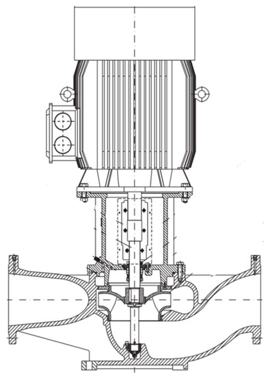
Figure 1.
Illustration of the experiment pump (vertical pipe pump).
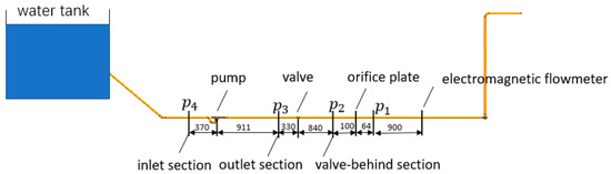
Figure 2.
Diagram of the experiment (units are mm).
The data are acquired with an NI-4497. The data acquisition frequency is 5000 Hz. The pump comprises the motor, pump body, impeller, and diffuser. The parameters for the pump are listed in Table 1. The pump is controlled by a frequency conversion cabinet. The data measurements mostly contain pressure sensor, electromagnetic flowmeter, and photoelectric speed sensor. In the experiment, the pump starts up first; meanwhile, the valve remains closed for a period of time, Tc, and then the valve is rapidly full opened.

Table 1.
Specifications for the experimental pump.
The installation locations of three pressure sensors are shown in Figure 2. The transient pressure at the inlet, outlet, and valve-behind section were measured.
The pump transported water from a tank to the atmosphere during the experiments. When the ball valve was fully opened, the flow rate was 0.0033 m3/s. Then, we changed the valve opening degree to adjust the flow rate to 0.0033, 0.00326, 0.00309, 0.0025, 0.00136, and 0 m3/s, respectively. The aim of the experiments was analyzing the steady performances at different flow rates. It took 9.1 s for the pump to reach 2900 rpm in this series of experiments.
The transient performances of the pump-valve system were studied by many experiments during the startup process. We started the pump first and then kept the valve closed until the pump’s rotational speed reached a certain value. The closed time for the valve was called Tc, and Tc was set as 0, 2.0, 3.2, 4.4, 5.9, 7.2, 8.0, 10.28, and 11.56 s, respectively. Then, at time point Tc, the valve was quickly opened in time To, and the data were collected until the pump reached the rated speed.
2.2. Processing the Experiment Data
A photoelectric speed sensor was used to measure the pump’s transient rotation speed. The photoelectric speed sensor outputs the pulse signal. The rotational speed used the pulses gathered in the time interval. The formula is expressed as:
where n is the transient speed and N is the number of pulses in .
The transient head could be calculated through measuring the transient pressure of the inlet section and outlet section, and the transient head also contained a component which was used to accelerate the fluid in the startup period.
where Leq is the equivalent length, P0 is the outlet pressure, Pi is the inlet pressure, and A is the cross-sectional area of the pipeline.
The dimensionless head and flow are defined as equaling:
where u2 = πd2Nr/60, Nr is the current rotational speed of the pump, b2 is the outlet width of the impeller, and d2 is the diameter of the impeller.
Transient flow is an important parameter in the startup period. The flow is mostly measured by an electromagnetic flowmeter and an orifice flowmeter. When measuring the transient flow, the electromagnetic flowmeter has a greater delay. Figure 3 is an illustration of the orifice flowmeter. Bernoulli equation and the continuity equation between the high pressure and orifice are used to obtain the flow. Formula (5) shows the flow transition equation:
where C is the outflow coefficient and β equals d/D.
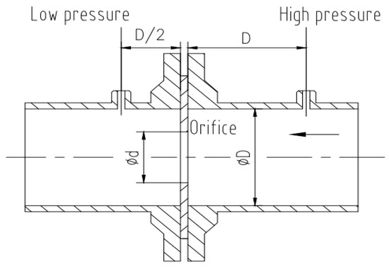
Figure 3.
Illustration of the orifice flowmeter.
The outflow coefficient C is used to correct the pressure difference between the orifice and the low pressure. Yet, the orifice flowmeter does not consider the pressure loss of the orifice. In this paper, the local resistance loss is used to get the flow. Formulas (6) and (7) show the energy conservation equation and the local resistance equation. The local resistance coefficient is influenced by the orifice structure and the Reynolds number. Thus, it can be found that the pressure difference is a quadratic function of the flow:
where is the resistance coefficient and is the equivalent length.
Figure 4a is a schematic diagram. The distance between the low pressure and the orifice plate is 6D, and between the high pressure and the orifice it is 3D. The pressure measuring point for the local resistance flowmeter should be in a stable flow area, while the low pressure point in the orifice flowmeter should be in an unstable area. An electromagnetic flowmeter was installed downstream to get a precise steady flow. The orifice plates come in three sizes, and ultimately the first one was chosen because it causes the biggest pressure loss; therefore, in the small flow we can get a more definitive pressure difference. The pump is controlled by the inverter, then a series of flowrates can be found by changing the frequency. Through a series of steady state experiments, the relationship of pressure difference and flowrate can be found. Figure 5 shows the fitting curve and fitting formula.
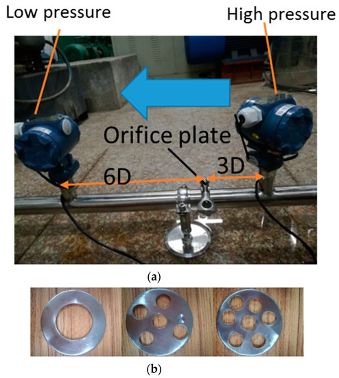
Figure 4.
Illustration of the local resistance flowmeter; (a) the schematic diagram, (b) three sizes for the orifice plate.
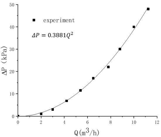
Figure 5.
The fitting curve of the pressure difference and flowrate.
2.3. Results and Discussion for the Experiment
The rotational speed is shown in Figure 6. The startup time for the pump was 9.1 s. Figure 7 shows the changes in pressure during the startup period.
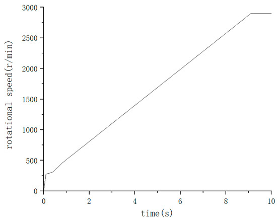
Figure 6.
The rotational speed of pump measured by the photoelectric speed sensor.
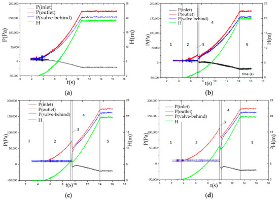
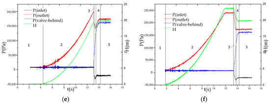
Figure 7.
The inlet pressure, outlet pressure, and pressure behind the valve under different Tc during the startup process; (a) Tc = 0 s, (b) Tc = 2.7 s, (c) Tc = 4.2 s, (d); Tc = 5.8 s, (e) Tc = 7.8 s, (f) Tc = 10.3 s.
The experimental process can be divided into five parts. Zone 1 means that the pump was stopped, zone 2 means that the pump was opened while the valve was closed, zone 3 means that the valve was opening, zone 4 means that the valve was fully opened, and zone 5 means that the pump system became stable. Tc is the closing time for the valve. Tc = 0 means that the valve was completely open during the pump startup period. When the valve was closed, the inlet pressure and pressure behind the valve remained unchanged, while the outlet pressure increased more rapidly than the operating condition at Tc = 0. The outlet pressure continued to increase more rapidly. When the valve was in the process of opening, the outlet pressure had a sudden fall in 0.4 s. Meanwhile, the pressure behind the valve increased rapidly and a pressure fluctuation occurred at the inlet of the pump. When the valve was completely open, the pressure behind the valve kept growing slower. Finally, the pressures in the different working conditions reached the same value. The outlet pressure was greater than the pressure behind the valve. This deviation could be caused by the resistance between the valve and pipe. There was a jump in the rotational speed curve at the initial stage of the start that does not match with the pressure curve and head curve. In the initial stages of startup, the energy provided by the centrifugal pump was smaller than the resistance of pipe system, and therefore the response could not have been sensitive to the pressure.
In order to compare different working conditions, the dimensionless flow and head were analyzed. Figure 8 shows the changes in dimensionless flow during the startup period. To is the startup time of the pump. The red curve is the startup period of the pump with a completely open valve. When the valve was closed, the dimensionless flow remained around 0. When the valve was opening, Cq rapidly increased and the curve rapidly tended to the red completely open curve. When Tc was less than To, the Cq first increased rapidly and then had a slow increment with the same tendency compared with the completely open startup period. When Tc was bigger than To, the Cq quickly increased to the final value.
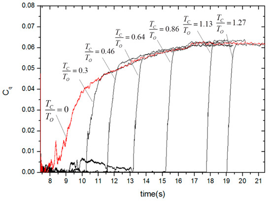
Figure 8.
Dimensionless flow for different startup periods.
Figure 9 shows the changes in the non-dimensional head during the startup period. The red curve is the startup period of the pump with a completely open valve. In the pump startup period, when the valve remained closed Ch was bigger than the completely open case. In the opening period of the valve, the Ch had a sudden drop and then tended to the completely open case rapidly. Finally, Ch in all those cases reached a certain value. When Tc divided by To was less than or equal to 0.46, the Ch reached the maximum when the pump was fully started. When Tc divided by To was greater than 0.46, the Ch reached the maximum at the point where the valve was going to open. When Tc was less than To, the maximum of Ch increased as Tc increased. When Tc was greater than To, the maximum of Ch maintained a certain value. If we want to achieve a high initial Ch, then Tc should be bigger than To.
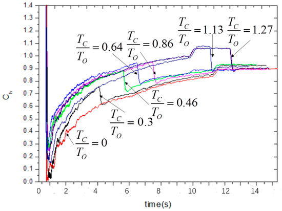
Figure 9.
Dimensionless head for different startup periods.
Considering the differential of the flow, Figure 10 shows the changes for different startup periods. The red curve is the startup period of the pump with a completely open valve. Figure 10b is the enlarged image of differential Q when Tc/To = 0; when the valve was completely open during the startup period, the dQ/dT increased to the maximum of about 2.25 and then fell to 1.25 or so, and finally the dQ/dT fell to 0. From Figure 6, it can be found that the rotational speed has a higher acceleration at first and then transitions to a certain smaller acceleration. The change in speed reflects the change in dQ/dT. Figure 10a shows the dQ/dT for different startup periods. During the valve’s opening period, the dQ/dT quickly reaches the maximum and then falls to the red curve, and finally tends to 0. When Tc is less than To, the maximum of dQ/dT increases when Tc increases. When Tc is bigger than To, the maximum of dQ/dT does not increase and even decreases a little when Tc increases. Thus, in order to obtain the biggest flow during a given short period of time, the Tc should be in the vicinity of 1.13 To, and there is no need to increase Tc when Tc is bigger than To.
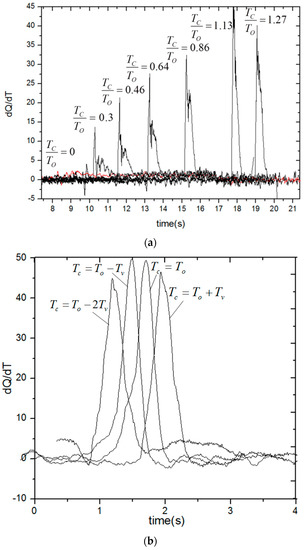
Figure 10.
Differential flow for different startup periods; (a) flow change rate (dQ/dT) for different startup periods; (b) flow change rate (dQ/dT) curve when Tc is in the vicinity of 1.13 To.
According to the above results, in order to find the most suitable Tc, a series of experiments when Tc is in the vicinity of 1.13 To have been performed. The results are shown in Figure 10b; it can be found that when Tc = To−Tv, the biggest flow can be found during a given short period of time.
3. Numerical Simulation
3.1. Computational Domain and Grid
The overall view of the 3D model is shown in Figure 2 and Figure 3. The numerical 3D model’s parameters were the same size as the real test system. The schematic view of numerical pump model and simplified valve model is shown in Figure 11. Table 2 shows the general view of the mesh of the pump-system model. The computational domain is discretized by an unstructured tetrahedral cell. The grid independence test is carried out, and Figure 12 shows the results. In the calculation, the scaled residuals of continuity equation and momentum equations are reduced to a magnitude below 10−5, and the scaled residuals of the turbulence kinetic energy (k) and dissipation rate (ξ) are reduced to a magnitude below 10−4. The y+ value near the critical surfaces is from 0 to 30 and the average value is within 50. The difference in head between the 1.98 × 10⁶ grid number and the 2.71 × 10⁶ grid number is 0.011%, and the difference in flow is 0.026%. As a result, the total number of grids is ensured to be 1.98 × 10⁶.
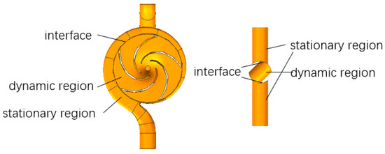
Figure 11.
The numerical model for the pump and ball valve.
Table 2.
Overview of the mesh in the numerical model.
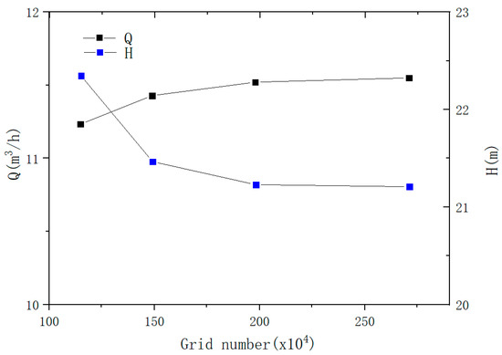
Figure 12.
Results of the grid independence investigation.
Steady simulations were performed firstly. The Q-H curve between the experiment and steady simulation is shown in Figure 13. The strong similarity in the results verifies the accuracy of the 3D model and grid quality. The flow in the follow-up experiment and transient simulation was around 0.003 m3/s.
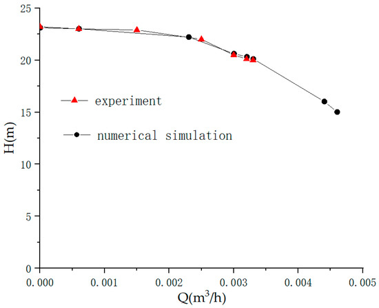
Figure 13.
Comparison of the experimental and steady numerical simulation.
3.2. Boundary Conditions of the Transient Simulation
The startup period of Tc = 8 s was simulated. Li [11] demonstrated the applicability of the detached eddy simulation (DES) model and the dynamic slip region (DSR) method in a transient simulation of the pump’s startup periods. For the DES (detached eddy simulation) model, in the attached boundary layer, the RANS equation is applied; the large eddy simulation (LES) model is applied in other regions. The LES is more precise and the RANS is more efficient, and the DES model integrates the advantages. Using the DES model can save computational resources and computing time to some extent.
The DSR (dynamic slip region) method segments the flow domain into dynamic and static regions. Then, the dynamic region and stationary region are discretized, respectively, and then a pair of interfaces is used to transfer and exchange data to the two individual parts. The interfaces could be set up in the fluent.
A mathematical curve is used to define the speed. It was achieved with measurements from the experiment. Figure 6 shows the rotational speed curve, and formula 8 (the unit is r/min) shows the definition of speed.
The valve’s opening time is 0.4 s, and valve’s rotational speed is assumed to be constant. Thus, the valve’s rotational speed can be defined as follows (the unit is degree/s):
In order to ensure both accuracy and efficiency, we set the time steps to vary with pump’s rotational speed. Thus, time step is also a value that varies with time. Formula 10 (the unit is s) shows the definition of the time step. At each time step, the blade does not rotate more than one degree when t ≤ 0.85 s, the blade does not rotate more than four degrees when 0.85 s < t ≤ 9.1 s, and then the blade does not rotate more than six degrees.
The boundary conditions of the pressure inlet and pressure outlet were chosen. Second-order implicit was applied for the time-dependent term format. The SIMPLEC algorithm was used to compute the pressure–velocity coupling. The dispersion of convective terms was calculated by the second-order upwind scheme, and the numerical under-relaxation and diffusion terms were calculated by central difference schemes.
There is an assumption that the water was incompressible in the numerical simulations at the startup period and there was no cavitation. The numerical simulation utilized Ansys Fluent.
3.3. Comparison of the Simulation and Experiment
Figure 14, Figure 15 and Figure 16 show the comparison of the transient simulation and the experiment. The experiment was recorded at Tc = 7.8 s, while the simulation was made at Tc = 8 s. The simulated pressure is probably about 2000 Pa higher than the experiment at the initial stage; this is caused by the measurement deviation in the water level in the tank. From the head and flow pictures, we can see that before the opening of the valve the simulation and experiment show a strong agreement, and the difference between the simulation and the experiment are mainly caused by a deviation of 0.2 s. In this experiment, the ball valve is controlled manually and the deviation is inevitable. Yet, the similarity between the numerical simulation and the experiment can prove the accuracy of the simulationn.
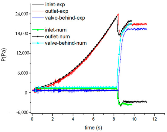
Figure 14.
Comparison of the experiment and simulation pressures.
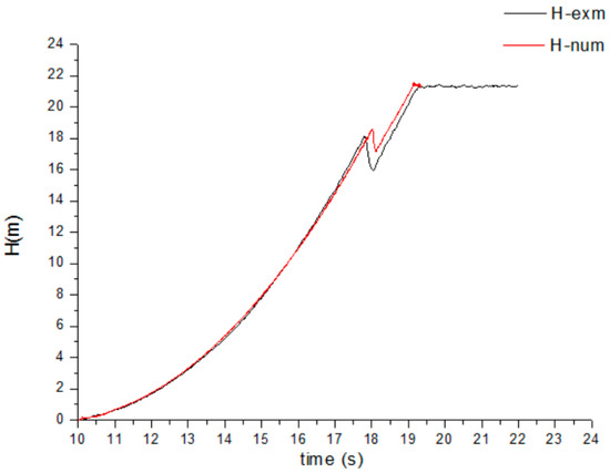
Figure 15.
Comparison of the experiment and simulation heads.
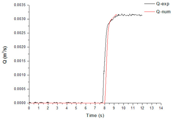
Figure 16.
Comparison of the experiment and simulation flows.
3.4. Results and Discussion of the Transient Simulation
The evolution of the velocity field at the opening period of valve is shown in Figure 17. A high-velocity zone appears at nearby of interface between valve and pipe when valve is opening. With the increase of opening degree, this high-velocity region decreases. The high-velocity region results in turbulence in the vicinity region, but there is little effect on the internal flow of pump because the valve’s inlet flow is generally uniform. The change in resistance has a greater impact on the transient internal flow of pump. The sudden drop in head and pressure occurred because the pump works on the domain behind the valve.
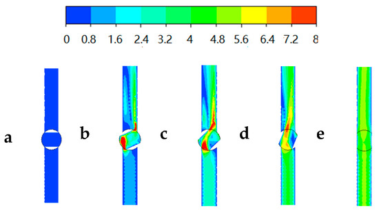
Figure 17.
The velocity evolution of the valve during the valve opening process: (a) t = 8 s, (b) t = 8.1 s, (c) t = 8.2 s, (d) t = 8.3 s, (e) t = 8.4 s.
The internal velocity evolution of pump during the opening period of valve is shown in Figure 18. In Figure 18a, it can be found that there is a clear vortex in volute tongue and trailing edge of blades. In Figure 18b,c, it can be found that the turbulence flow occurs in the leading edge of the blades. In Figure 18e, the pump’s internal flow structure changes back to a representative transient flow structure when the valve is fully open. During the valve’s opening period, the vortexes in the trailing edge of the blades and the volute tongue gradually disappears. In the valve’s opening period, the performance of the pump has been improved. When the valve is closed, the pump’s performance is weakened. This might be the reason why the maximum of flow change rate (dQ/dT) does not increase and even decreases a little, while Tc increases when Tc is bigger than To.
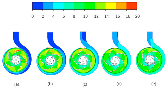
Figure 18.
The internal velocity evolution of the pump during the valve opening process: (a) t = 8 s, (b) t = 8.1 s, (c) t = 8.2 s, (d) t = 8.3 s, (e) t = 8.4 s.
4. Conclusions
The research emphasis was a pump-valve system (centrifugal pump and ball valve). Many experiments and numerical simulations were carried out to study the transient performances of the pump-valve system. The study of transient performance mainly focused on how to get a large fluid acceleration.
In the experiments, the local resistance loss was used to measure the transient flow more accurately. The results of experiments show that a high and rapid transient response can be achieved by controlling the assistant valve during the pump’s startup period. When Tc > To, the maximum of dQ and Ch will not increase. Thus, the most suitable startup method for the pump and valve will be around Tc = To. Based on the experimental results, when Tc = To − Tv the biggest flow can be obtained during a given short period of time. Thus, the suggested suitable startup method for the pump and valve is Tc = To − Tv, which can get the biggest flow and a lower max pressure.
The most suitable Tc is noted by considering the transient response’s sensitivity and stability synthetically. When the most suitable Tc is determined by the experiments, a numerical simulation is carried out to study the internal flow. The dynamic movement of the impeller and the valve is defined by the DSR method. The transient numerical simulation uses the DES model. The simulated results and experimental results show a good agreement. The simulation predicts the pressure and head volatility because of the valve’s sudden opening. During the valve’s opening period, the impeller-volute interaction plays a decreasing role in the pump’s performance, while the vortex’s revolution plays an increasing role. During the opening period of valve, the change in the valve resistance influences the internal flow of the pump.
This paper only investigated the consequence of Tc. Others are involved in the matching method, such as the valve degree. The key point of future work will be to study these factors synthetically and find the best matching mode.
Author Contributions
Conceptualization, Q.L. and P.W.; methodology, Q.L.; software, Q.L. and S.Y.; validation, Q.L., D.W., and X.M.; formal analysis, Q.L.; investigation, Q.L.; resources, D.W. and X.M.; data curation, Q.L.; writing—original draft preparation, Q.L.; writing—review and editing, P.W. and B.H.; supervision, P.W. and B.H.; project administration, P.W. and X.M.; funding acquisition, D.W. All authors have read and agreed to the published version of the manuscript.
Funding
This study was supported by the National Natural Science Foundation of China (No. 51839010, No. 52076186).
Acknowledgments
The author sincerely thanks the support of the State Key Laboratory of Fluid Power Transmission and Control of Zhejiang University.
Conflicts of Interest
The authors declare no conflict of interest.
Nomenclature
| H | Total head (m) |
| Q | Volume flow rate (m3/s) |
| Speed | The rotational speed of the pump (r/min) |
| The speed of the ball valve (degree/s) | |
| P | Pressure (Pa) |
| Tc | The closed time of the valve (s) |
| To | The opening time of the pump (s) |
| Tv | The opening time of the valve (s) |
| Ch | The non-dimension head |
| Cq | The non-dimension flow |
| u2 | Outlet peripheral velocity of the impeller (m/s) |
| b2 | The outlet width of impeller (mm) |
| d2 | The diameter of impeller (mm) |
| Re | Reynolds number |
References
- Lefèbvre, P.J.; Barker, W.P. Centrifugal Pump Performance during Transient Operation. J. Fluids Eng. 1995, 117, 123–128. [Google Scholar] [CrossRef]
- Tsukamoto, H.; Ohashi, H. Transient Characteristics of a Centrifugal Pump during Starting Period. J. Fluids Eng. 1982, 104, 6–13. [Google Scholar] [CrossRef]
- Tsukamoto, H.; Matsunaga, S.; Yoneda, H.; Hata, S. Transient Characteristics of a Centrifugal Pump during Stopping Period. J. Fluids Eng. 1986, 108, 392–399. [Google Scholar] [CrossRef]
- Saito, S. The Transient Characteristics of a Pump during Start Up. Bull. JSME 1982, 25, 372–379. [Google Scholar] [CrossRef]
- Wu, D. Study on Transient Characteristics of Special-Type Centrifugal Pump during Rapid Starting Period. Ph.D. Thesis, Zhejiang University, Hang Zhou, China, 2004. [Google Scholar]
- Wu, D.Z.; Wang, L.Q.; Hu, Z.Y. Numerical simulation of centrifugal pump’s transient performance during rapid starting period. J. Zhejiang Univ. Eng. Sci. 2005, 39, 1427–1430, 1454. [Google Scholar]
- Dazin, A.; Caignaert, G.; Bois, G. Transient Behavior of Turbomachineries: Applications to Radial Flow Pump Startups. J. Fluids Eng. 2007, 129, 1436–1444. [Google Scholar] [CrossRef]
- Wang, L.Q.; Wu, D.Z.; Zheng, S.Y.; Hu, Z.Y. Study on transient hydrodynamic performance of Mixed-Flow-Pump during starting period. J. Zhejiang Univ. Eng. Sci. 2004, 38, 751–755. [Google Scholar]
- Wu, D.; Chen, T.; Sun, Y.; Cheng, W.; Wang, L. Study on numerical methods for transient flow induced by speed-changing impeller of fluid machinery. J. Mech. Sci. Technol. 2013, 27, 1649–1654. [Google Scholar] [CrossRef]
- Wu, D.; Chen, T.; Sun, Y.; Li, Z.; Wang, L. A study on numerical methods for transient rotating flow induced by starting blades. Int. J. Comput. Fluid Dyn. 2012, 26, 297–312. [Google Scholar] [CrossRef]
- Li, Z.; Wu, D.; Wang, L.; Huang, B. Numerical Simulation of the Transient Flow in a Centrifugal Pump During Starting Period. J. Fluids Eng. 2010, 132, 081102. [Google Scholar] [CrossRef]
- Li, Z.; Wu, P.; Wu, D.; Wang, L. Experimental and numerical study of transient flow in a centrifugal pump during startup. J. Mech. Sci. Technol. 2011, 25, 749–757. [Google Scholar] [CrossRef]
- Chern, M.-J.; Wang, C.-C.; Ma, C.-H. Performance test and flow visualization of ball valve. Exp. Therm. Fluid Sci. 2007, 31, 505–512. [Google Scholar] [CrossRef]
- Yang, Q.; Zhang, Z.; Liu, M.; Hu, J. Numerical Simulation of Fluid Flow inside the Valve. Procedia Eng. 2011, 23, 543–550. [Google Scholar] [CrossRef]
- Wang, L.; Song, X.G.; Park, Y.C. Dynamic analysis of three-dimensional flow in the opening process of a single-disc butterfly valve. J. Mech. Eng. Sci. 2010, 224, 329–336. [Google Scholar] [CrossRef]
- Cho, T.-D.; Yang, S.-M.; Lee, H.-Y.; Ko, S.-H. A study on the force balance of an unbalanced globe valve. J. Mech. Sci. Technol. 2007, 21, 814–820. [Google Scholar] [CrossRef]
- Srikanth, C.; Bhasker, C. Flow analysis in valve with moving grids through CFD techniques. Adv. Eng. Softw. 2009, 40, 193–201. [Google Scholar] [CrossRef]
- Nguyen, Q.K.; Jung, K.H.; Lee, G.N.; Suh, S.B.; To, P. Experimental Study on Pressure Distribution and Flow Coefficient of Globe Valve. Processes 2020, 8, 875. [Google Scholar] [CrossRef]
© 2020 by the authors. Licensee MDPI, Basel, Switzerland. This article is an open access article distributed under the terms and conditions of the Creative Commons Attribution (CC BY) license (http://creativecommons.org/licenses/by/4.0/).