Bi-Level Model Predictive Control for Optimal Coordination of Multi-Area Automatic Generation Control Units under Wind Power Integration

Abstract

With the high degree of wind power penetration integrated into multi-area AC/DC interconnected power grids, the frequency regulation capacity of automatic generation control (AGC) units is not sufficient in the wind power-penetrated area, making it difficult to effectively suppress the frequency stability caused by the fluctuation of wind power. Therefore, a coordinated control strategy for AGC units across areas based on bi-level model predictive control is proposed in this paper to achieve resource sharing. The control scheme uses economic model predictive control to realize steady power optimal allocation of the AGC units across areas in the upper layer and distributed model predictive control to realize dynamic frequency optimization control of the multi-area AGC units in the lower layer. Taking a three-area AC/DC interconnected power grid with a wind farm as an example, the simulation results show that, compared with model predictive control using tie-line frequency bias control (TBC) mode, the proposed control strategy can not only effectively maintain tie-line safety and frequency stability, but can also reduce the regulation cost of multi-area AGC units.

1. Introduction

With the gradual expansion of the grid-connected capacity of renewable energy sources, such as wind power and photovoltaics, the intermittent and stochastic volatility of their output power has brought huge scheduling and control pressure to the frequency stability of power systems [1]. On the one hand, each control area performs zoning control according to the AC/DC tie-line transmission plan. Each control area can only cover its own power imbalance and maintain the planned power exchanges of the tie-lines, thus it cannot support other areas of regulation capacity shortages through the tie-lines [2,3]. On the other hand, the multi-area AGC units are not taken as a whole to suppress the total power fluctuation. Therefore, making full use of the ability of transregional AC/DC tie-line transmission to achieve multi-area coordination has become a major concern for the secure operation of multi-area interconnected power systems [4].

AGC units act as an important regulation resource for energy management systems (EMSs) and are responsible for balancing the total power fluctuations caused by load and renewable energy in real time. At present, the control mode of AGC units is tie-line frequency bias control (TBC) mode [5]. TBC control mode requires the AGC units of each control area to only respond to disturbances in their own area and not participate in the regulation of other areas. The biggest advantage of this is that power disturbances are locally balanced; however, when the regulation capacity of a disturbed area is insufficient, the frequency of the disturbed area can become unstable. The optimal coordination of multi-area AGC units can realize sharing of all regulation resources and inter-area power support through the AC/DC tie-line [6,7].

In recent years, many advanced control schemes have been applied to design a control system for multi-area AGC units, such as the intelligent optimization control method, which is widely used due to its simple control structure for effectively optimizing the parameters of proportional-integral-derivative (PID) controllers. However, intelligent optimization methods—such as particle swarm optimization (PSO) [8], ant lion optimizer algorithm (ALO) [9], imperialist competitive algorithm (ICA) [10], grey wolf optimizer algorithm (GWO) [11], and so on—may become trapped at local minima, leading to worse dynamic response performance. In order to overcome this deficiency, model predictive control (MPC) [12] has become a promising research interest over the past decade and has been applied to the design of a control system for multi-area AGC units. In [13], the authors recalled some achievements of MPC over the past decades, and in [14], some guides to design MPC controllers using MATLAB were presented. A comparison between MPC and conventional PI control in AGC system design was made in [15] to demonstrate the benefits of MPC, such as having flexibility and coordination between multiple inputs, taking into account system limitations, and exploiting knowledge about disturbances acting on the system. In [16], the authors studied the merging of wind turbines in a multi-area power system controlled by a robust AGC based on the MPC technique. In [17], the parameters of the MPC controller were determined by a bat-inspired algorithm to deal with system nonlinearities comprising generation rate constraints (GRCs) and governor dead bands (GDBs). However, these centralized control solutions are often impractical for application to a large-scale power system for computational reasons and the lack of error tolerance. When the centralized MPC controller or a control component fails, the entire AGC system gets out of control, and the control integrity cannot be guaranteed [18]. The distributed MPC approach, whereby each control area is controlled by an independent MPC controller, has the advantages of error tolerance, less computational effort, and flexibility regarding the AGC system structure. A distributed MPC approach with a terminal state penalty for multi-area power systems was presented in [19], but did not consider the system constraints. In [20], a distributed MPC technique was presented for a multi-area interconnected power system, in which the distributed MPC controllers coordinated with each other by exchanging their information. In [21], the authors proposed a distributed MPC scheme for a four-area hydrothermal interconnected power system, in which the limit position of the governor valve was modeled by a fuzzy model and the local predictive controllers were incorporated into the nonlinear control system. In order to better deal with the constraints, a distributed MPC was proposed in [22] based on discrete-time Laguerre functions for multi-area interconnected power systems. Moreover, a multi-area AGC dynamic model integrated with a simplified wind turbine model was solved by a distributed MPC approach in [23]. In [24], the authors proposed a coordinated distributed MPC for an AGC system that included inherently variable wind-power generation.

However, to the best of our knowledge, while these distributed MPC methods can reduce the AGC regulation resource demands of the entire power system [25], they cannot effectively improve the economics of AGC units while ensuring AC tie-line safety. In addition, a great deal of attention has been paid to AC interconnections between areas but not to AC/DC parallel interconnections between areas [26,27]. In this paper, a two-level hierarchical control framework is proposed to guarantee the safety of AC/DC tie-lines and reduce the cost of cross-regional support, and further, to achieve better frequency control performance for multi-area interconnected systems. The innovations of the proposed control approach are described as follows: the control framework of the proposed method consists of two layers, with a steady-state power allocation layer at the upper level and a dynamic frequency control layer at the lower level. The upper-level economic MPC (EMPC) controller is used to realize the steady-state power optimal allocation of multi-area AGC units under tie-line support constraints. The AGC units’ participation factors are sent to each control area through the steady-state power allocation layer. The lower-level distributed MPC (DMPC) controller is used to realize dynamic frequency optimization control of the multi-area interconnected system. The control signals of the distributed MPC controller are acted on each control area through the dynamic frequency control layer, so that the area error signal can be restored to zero. This bi-level model predictive control (BMPC) method optimizes the steady-state power and dynamic frequency control of cross-regional AGC units progressively, which can effectively guarantee the safety and economy of optimal cooperation frequency control of multi-area AGC units.

The remainder of this paper is organized as follows. An AGC model of a multi-area power system with a wind farm is established in Section 2. Subsequently, in Section 3, the systematic formulation of the BMPC for multi-area AGC units is developed, which consists of two layers, with the steady-state power allocation layer at the upper level and the dynamic frequency control layer at the lower level. Then, in Section 4, case studies on a three-area AC/DC interconnected power grid are conducted to validate the better performance of the proposed BMPC method. Finally, some concluding remarks are presented in Section 5.

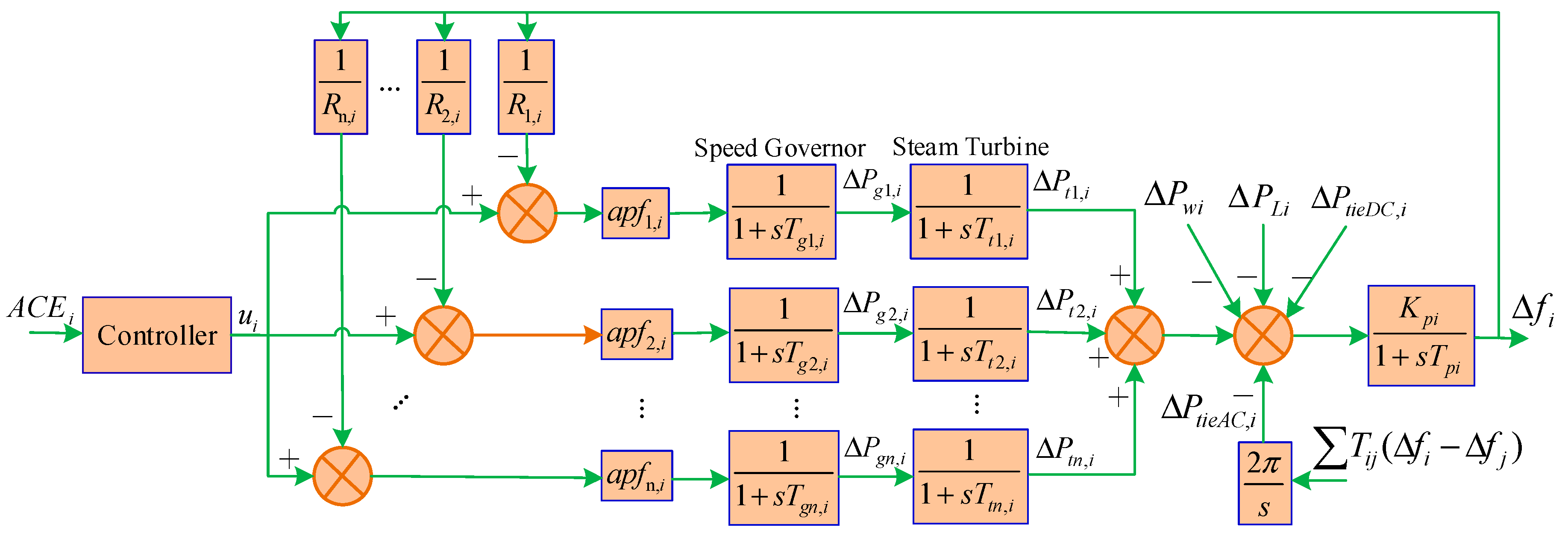
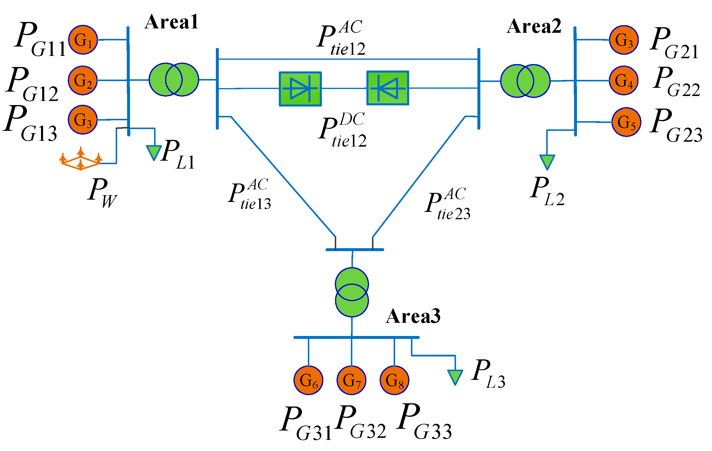
2. Automatic Generation Control Model of Multi-Area Power System with Wind Farm

Automatic generation control of the multi-area interconnected power system is required to keep the balance between generation and load. Whenever the balance is broken by any sudden change in local load and wind power output, the controller of each control area i is responsible for manipulating the AGC units to force the frequency deviations and tie-line power flow deviations to zero. Since the range of load variance is small during its normal operation, the AGC system model of the multi-area power system can be linearized around the stable operation point [28]. In this paper, the AGC model of control area i shown in Figure 1 is adopted, consisting of governor module, turbine module, rotating mass-load module, AC/DC tie-line module, wind farm module, controller, and so on. The meanings of symbols of state space variables used in Figure 1 are given in

Table 1. Meanings of symbols of state space variables.

Symbol	Name of Parameter/Constant
$\Delta f_i$	Incremental frequency deviation of area i
$\Delta P_{tieAC,i}$	Total AC tie-line power change between area i and other areas
$\Delta P_{tieDC,i}$	Total DC tie-line power change between area i and other areas
$\Delta P_{wi}$	Wind farm disturbance signal of area i
$\Delta P_{Li}$	Load disturbance signal of area i
$K_{pi}$	Gain constant of power system of area i
$T_{pi}$	Time constant of power system of area i
$T_{ij}$	AC tie-line synchronizing coefficient between area i and area j
$AC{E}_i$	Area control error of area i
$u_i$	Input control signal from controller of area i
$R_{k,i}$	Droop characteristic coefficient
$T_{gk,i}$	Steam turbine governor time constant
$T_{tk,i}$	Steam turbine time constant
$\Delta P_{tk,i}$	Power incremental change
$\Delta P_{gk,i}$	Governor-valve position incremental change
$ap{f}_{k,i}$	AGC unit participation factor

.

The transfer function model described in [29] is adopted to represent the high voltage direct current (HVDC) link in Figure 1, where the HVDC link is considered to be operated in constant current control mode, and the incremental power flow through the link is modelled with incremental change in frequency at the rectifier end [30]. For small-load perturbation HVDC tie-line flow, $\Delta P_{tieDC,ij}$ is given by

$$\Delta P_{tieDC,ij}=\frac{K_{dc}}{1+s{T}_{dc}}(\Delta f_i-\Delta f_j),$$

(1)

where $K_{dc}$ denotes HVDC modulation coefficients and $T_{dc}$ represents the delay in establishing the HVDC current after a small load disturbance. Therefore, Equation (1) can be rewritten as

$$\Delta {\dot{P}}_{tieDC,ij}=-\frac{\Delta P_{tieDC,ij}}{T_{dc}}+\frac{K_{dc}}{T_{dc}}(\Delta f_i-\Delta f_j),$$

(2)

and the total DC tie-line power change between area i and other areas is calculated as

$$\Delta P_{tieDC,i}={\displaystyle \sum _{j\in i,j\ne i}\Delta P_{tieDC,ij}}.$$

(3)

The area control error (ACE) of control area i can be expressed as

$$AC{E}_i={\beta }_i\Delta f_i+(\Delta P_{tieAC,i}+\Delta P_{tieDC,i}),$$

(4)

where ${\beta }_i$ is the frequency-biasing factor.

According to the transfer function block diagram of the AGC control model with a wind farm depicted in Figure 1, the above frequency response model for area i can be described as the following state space model

$$\{\begin{array}{l}{\mathit{x}}_i(t)={\overline{\mathit{A}}}_{ii}{\mathit{x}}_i(t)+{\overline{\mathit{B}}}_{ii}{\mathit{u}}_i(t)+{\overline{\mathit{E}}}_i{\mathit{d}}_i(t)+{\displaystyle \sum _{j=1,j\ne i}^N({\overline{\mathit{A}}}_{ij}{\mathit{x}}_j(t)+{\overline{\mathit{B}}}_{ij}{\mathit{u}}_j(t))}\\ {\mathit{y}}_i(t)={\overline{\mathit{C}}}_i{\mathit{x}}_i(t)\end{array},$$

(5)

with

$${\overline{\mathit{A}}}_{ii}=\left[\begin{array}{cccccccc}-\frac{1}{T_{g1,i}}& 0& \cdots & 0& 0& 0& 0& -\frac{1}{T_{g1,i}{R}_{1,i}}\\ \frac{1}{T_{t1,i}}& -\frac{1}{T_{t1,i}}& \cdots & 0& 0& 0& 0& 0\\ ⋮& ⋮& ⋮& ⋮& ⋮& ⋮& ⋮& ⋮\\ 0& 0& \cdots & -\frac{1}{T_{gn,i}}& 0& 0& 0& -\frac{1}{T_{gn,i}{R}_{n,i}}\\ 0& 0& \cdots & \frac{1}{T_{tn,i}}& -\frac{1}{T_{tn,i}}& 0& 0& 0\\ 0& 0& \cdots & 0& 0& 0& 0& {\displaystyle \sum _{j=1,j\ne i}^{n}2\pi T_{ij}}\\ 0& 0& \cdots & 0& 0& 0& -\frac{1}{T_{dc}}& \frac{K_{dc}}{T_{dc}}\\ 0& \frac{K_{pi}}{T_{pi}}& \cdots & 0& \frac{K_{pi}}{T_{pi}}& -\frac{K_{pi}}{T_{pi}}& -{\displaystyle \sum _{j=1,j\ne i}^n\frac{K_{pi}}{T_{pi}}}& -\frac{1}{T_{pi}}\end{array}\right],{\overline{\mathit{B}}}_{ii}=\left[\begin{array}{c}\frac{ap{f}_{1,i}}{T_{g1,i}}\\ 0\\ ⋮\\ \frac{ap{f}_{n,i}}{T_{gn,i}}\\ 0\\ 0\\ 0\\ 0\end{array}\right],$$

(6)

$$\begin{gathered} {\overline{\mathit{E}}}_i=\left[\begin{array}{cc}0& 0\\ 0& 0\\ ⋮& ⋮\\ 0& 0\\ 0& 0\\ 0& 0\\ 0& 0\\ -\frac{K_{pi}}{T_{pi}}& -\frac{K_{pi}}{T_{pi}}\end{array}\right],{\overline{\mathit{A}}}_{ij}=\left[\begin{array}{cccccccc}0& 0& \cdots & 0& 0& 0& 0& 0\\ 0& 0& \cdots & 0& 0& 0& 0& 0\\ ⋮& ⋮& ⋮& ⋮& ⋮& ⋮& ⋮& ⋮\\ 0& 0& \cdots & 0& 0& 0& 0& 0\\ 0& 0& \cdots & 0& 0& 0& 0& 0\\ 0& 0& \cdots & 0& 0& 0& 0& -{\displaystyle \sum _{j=1,j\ne i}^{n}2\pi T_{ij}}\\ 0& 0& \cdots & 0& 0& 0& 0& -\frac{K_{dc}}{T_{dc}}\\ 0& 0& \cdots & 0& 0& 0& {\displaystyle \sum _{j=1,j\ne i}^n\frac{K_{pi}}{T_{pi}}}& 0\end{array}\right], \\ {\overline{\mathit{B}}}_{ij}=\mathit{O}, \end{gathered}$$

(7)

$${\overline{\mathit{C}}}_i=\left[\begin{array}{cccccccc}0& 0& \cdots & 0& 0& 1& {\displaystyle \sum _{j=1,j\ne i}^{n}1}& {\beta }_i\end{array}\right].$$

(8)

where ${\mathit{x}}_i={[\Delta P_{g1,i},\Delta P_{t1,i},\cdots ,\Delta P_{gn,i},\Delta P_{tn,i},\Delta f_i,\Delta P_{tieAC,i},\Delta P_{tieDC,i}]}^{\mathrm{T}}$ is the state vector of area i, ${\mathit{u}}_i=\Delta P_{ci}$ is the control input, ${\mathit{d}}_i={[\Delta P_{Li},\Delta P_{wi}]}^{\mathrm{T}}$ is the disturbance input, and ${\mathit{y}}_i$ is $AC{E}_i$ in area i, which is taken as the output of the system.

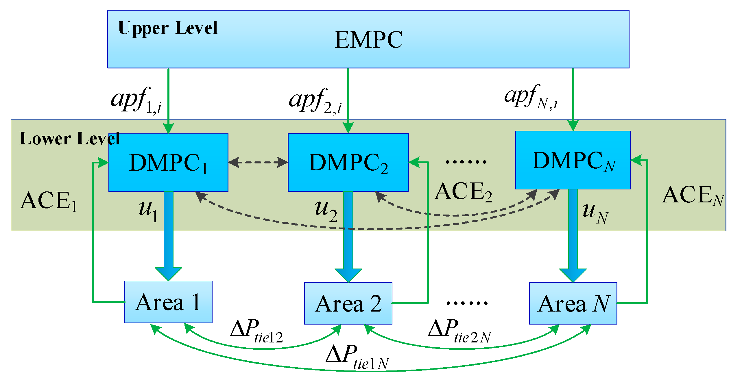
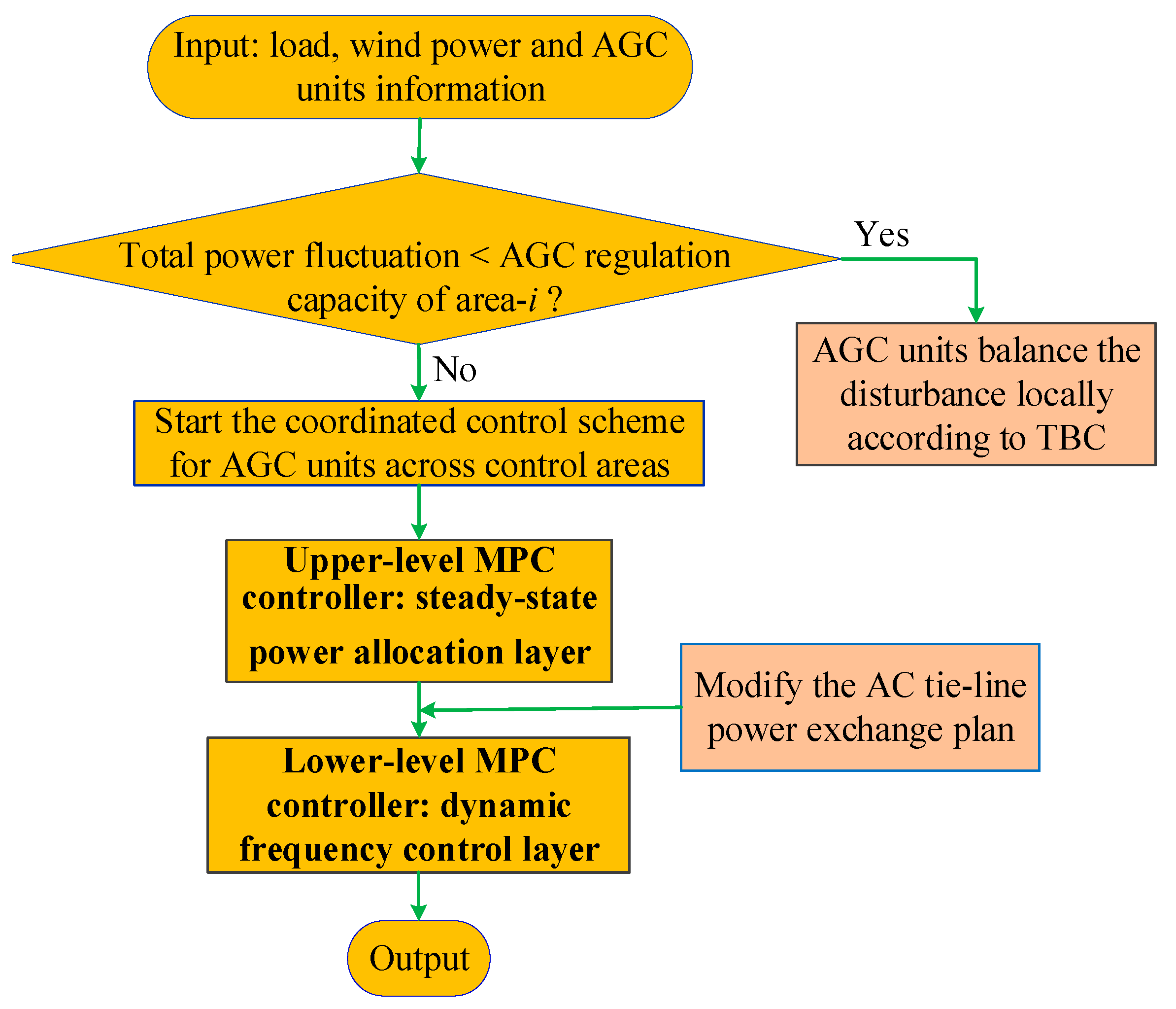
3. Coordinated Control Strategy for Automatic Generation Control Units Based on Bi-Level Model Predictive Control

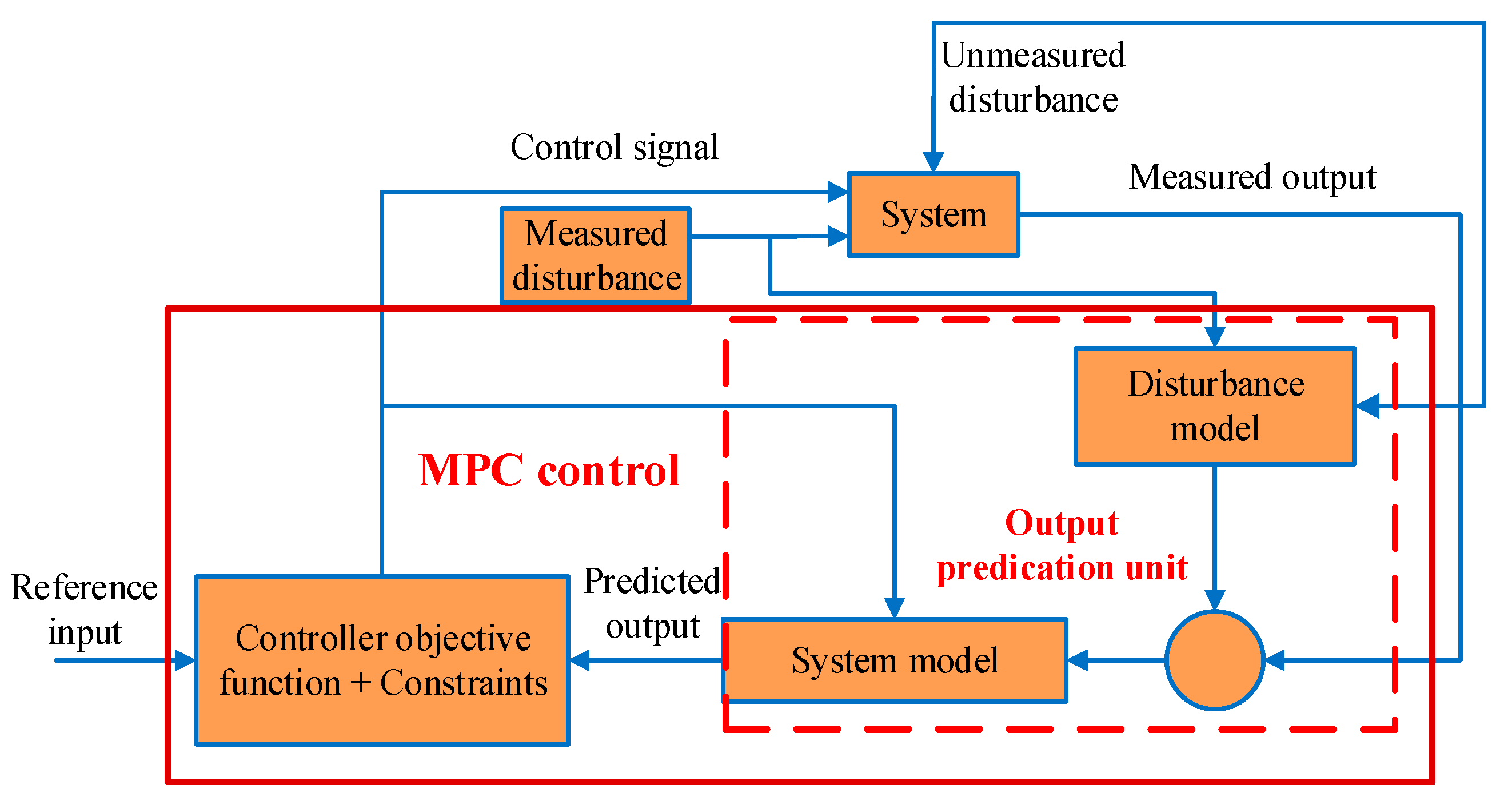
3.1. Bi-Level Model Predictive Control Framework

MPC has proved to be an effective approach to deal with large multivariable constrained control problems in industry [13], such as chemical processes, the petrol industry, power systems, and many other applications. The main idea of MPC is to choose control actions by repeatedly solving an online constrained optimization problem, which aims at minimizing a performance index over a finite prediction horizon based on predictions. Figure 2 gives a general structure of the MPC scheme. It comprises three components:

• A model of the system. This model is used to predict the future evolution of the system in an open loop, and the efficiency of the calculated control actions of an MPC highly depends on the accuracy of the model.
• A performance index over a finite horizon. This index will be minimized subject to constraints imposed by the system model, restrictions on control inputs and system state, and other considerations at each sampling time to obtain a trajectory of future control inputs.
• A receding horizon scheme. This scheme introduces the notion of feedback into the control law to compensate for disturbances and modeling errors.

MPC displays its main strengths in its computational expediency, real-time applications, and intrinsic compensation for treatment of constraints and potential for future extensions of the method. At each control interval, the first input in the optimal sequence is sent to the plant, and the entire calculation is repeated at subsequent control intervals.

With the rapid development of MPC theory, the MPC controller has developed from a single-layer to a double-layer control structure [31]. Methods of the single-layer control structure mainly consist of centralized MPC, decentralized MPC [32,33], and distributed MPC. MPC methods of double-layer control structure are optimized progressively between upper and lower level to achieve steady-state target tracking and dynamic optimal control [34].

In this paper, a two-level hierarchical control framework is proposed to guarantee the safety of AC/DC tie-lines and reduce the cost of cross-regional support, and further, to achieve better frequency control performance for multi-area interconnected systems. The control scheme divides economic optimization and process control into two layers: the upper layer adopts the EMPC to realize steady power optimal allocation of the multi-area AGC units, and the lower layer adopts the DMPC to realize dynamic frequency optimization control, which is shown in Figure 3. The upper-level EMPC controller decides the AGC units’ participation factors, which are sent down to each control area. The lower-level MPC controller realizes dynamic frequency optimization control of a multi-area interconnected system. The control signals of the DMPC controller are acted on each control area. This bi-level model predictive control method optimizes the steady-state power and dynamic frequency control of cross-regional AGC units progressively, which can effectively guarantee the safety and economy of optimal cooperation frequency control of multi-area AGC units.

3.2. Upper-Level Model Predictive Control Controller: Steady-State Power Allocation Layer

In this section, we focus on the design of the upper-level MPC controller. The aim of the steady-state power allocation layer is to cooperate with the AGC units of each control area to achieve economic and safety performance indicators, and its output is used as an optimal operating set-point for the lower-level MPC controller. Based on the ultra-short-term load forecasting and wind farm prediction information, we can obtain the total power fluctuation amount. It is balanced by the AGC units in the whole interconnected system according to the economic principle of incremental adjustment cost. Therefore, the upper-level MPC controller optimizes the incremental adjustment cost to adjust the power allocation factor of the AGC units in each control area.

According to the regulation capacity of the AGC units of area i, the steady-state power allocation layer is designed in two scenarios. The first scenario is where the regulation capacity of the AGC units of area i is sufficient; the total power fluctuation is balanced locally according to the TBC mode. Therefore, the steady-state power allocation layer can conduct economic power allocation based on the traditional equal incremental method. The second scenario is where the AGC units of area i have insufficient regulation capacity; the AC tie-line transaction protocol is modified to achieve cross-regional optimal allocation of total power fluctuations. This paper focuses on how to optimize the power allocation of the cross-regional AGC units.

The vector of state variables $\mathit{x}(k)$ is composed of the output of each AGC unit and AC tie-line exchange power, namely $\mathit{x}(k)={[P_{Gi,1}(k),P_{Gi,2}(k),\cdots ,P_{tieAC,mi}(k),\cdots ]}^{\mathrm{T}}$. In this paper, we assume that the power support transmitted across the areas is completed by the AC tie-lines and do not consider transmission losses. This is because the HVDC link usually operates at constant power. The vector of control variable $\mathit{u}(k)$ is formed by the incremental output of the multi-area AGC units, i.e., $\mathit{u}(k)={[\Delta P_{Gi,1}(k),\Delta P_{Gi,2}(k),\cdots ,\Delta P_{Gm,1}(k),\cdots ]}^{\mathrm{T}}$. The AC tie-line exchange power incremental is the output variable. According to the power balance equation of each period, the discrete state space model of the power balance equation can be formulated as

$$\{\begin{array}{l}\mathit{x}(k+\Delta t)=\left(\begin{array}{c}{P}_{Gi,1}(k+\Delta t)\\ P_{Gi,2}(k+\Delta t)\\ ⋮\\ P_{tieAC,mi}(k+\Delta t)\\ ⋮\end{array}\right)=\left[\begin{array}{ccccc}1& 0& \cdots & 0& \cdots \\ 0& 1& \cdots & 0& \cdots \\ 0& 0& \ddots & \cdots & \cdots \\ 0& 0& \cdots & 1& \cdots \\ 0& 0& \cdots & \cdots & \ddots \end{array}\right]\left(\begin{array}{c}{P}_{Gi,1}(k)\\ P_{Gi,2}(k)\\ ⋮\\ P_{tieAC,mi}(k)\\ ⋮\end{array}\right)+\left(\begin{array}{ccc}1& 0& \cdots \\ 0& 1& \cdots \\ 0& 0& \ddots \\ 1& 1& \cdots \\ ⋮& ⋮& \ddots \end{array}\right)\left(\begin{array}{c}\Delta P_{Gi,1}(k)\\ \Delta P_{Gi,2}(k)\\ ⋮\\ \Delta P_{Gm,1}(k)\\ ⋮\end{array}\right)\\ y_m(k)=\Delta P_{tieAC,mi}(k)=P_{tieAC,mi}(k+\Delta t)-P_{tieAC,mi}(k)={\displaystyle \sum _{j\in m}\Delta P_{Gm,j}(k)}\end{array}$$

(9)

Based on the discrete state space model (Equation (9)), the output $y_m(k+h\Delta t|k)$ in the prediction horizon at sample $k$ can be predicted; $h\in (1,P_u)$, $P_u$ is the prediction time domain. When the regulating capacity of AGC units is insufficient, the incremental cost of system operation is mainly composed of the incremental costs of multi-area AGC units and AC tie-line regulation. Therefore, the steady-state optimization objective at a control time domain is constructed as

$$J_u(k)={\displaystyle \sum _{h=1}^{P_u}\left[{\displaystyle \sum _{i\in N}{\displaystyle \sum _{j\in i}(K_f+K_e)S_{i,j}(\Delta P_{Gi,j}(k+h\Delta t|k))}}+{\displaystyle \sum _{m\in i,m\ne i}{D}_{mi}(\Delta P_{tieAC,mi}(k+h\Delta t|k))}\right]},$$

(10)

where N is the number of control areas; $S_{i,j}(\Delta P_{Gi,j})=a_{i,j}\Delta P_{Gi,j}^2+b_{i,j}\Delta P_{Gi,j}+c_{i,j}$ is the consumption characteristic of an AGC unit; and $a_{i,j}$, $b_{i,j}$, and $c_{i,j}$ are constant coefficients. $K_f$ and $K_e$ are the fuel price and CO₂ price, respectively. $\Delta P_{tieAC,mi}$ denotes the additional power transmission through AC tie-line $mi$, $D_{mi}(\Delta P_{tieAC,mi})=K_{ac}\Delta P_{tieAC,mi}$ is the power regulation cost of the AC tie-line, and $K_{ac}$ is the unit regulation cost of AC tie-line transmission power.

At instant k, the steady-state power allocation layer obtains the control sequence of the AGC units at a future time by solving the cost function (10)

$$\underset{\Delta P_{Gi}(k+h\Delta t|k)}{\min }{J}_u(k),$$

(11)

subject to

$${\displaystyle \sum _{j\in i}\Delta P_{Gi,j}}(k+h\Delta t|k)=\Delta P_{Li}(k+h\Delta t|k)+\Delta P_{wi}(k+h\Delta t|k)-{\displaystyle \sum _{m\in i,m\ne i}\Delta P_{tieAC,mi}(k+h\Delta t|k)},$$

(12)

$$\Delta P_{Gi,j}^{\min }\le \Delta P_{Gi,j}(k+h\Delta t|k)\le \Delta P_{Gi,j}^{\max },$$

(13)

$$\Delta P_{tieAC,mi}^{\min }\le \Delta P_{tieAC,mi}(k+h\Delta t|)\le \Delta P_{tieAC,mi}^{\max }.$$

(14)

where (12) is the real-time power balance equation; $\Delta P_{wi}(k+h\Delta t|k)$ is the deviation between predicted and actual value; $\Delta P_{Gi,j}^{\max }$ and $\Delta P_{Gi,j}^{\min }$ represent the upper and lower limits of the regulation capacity of the AGC unit, respectively; and $\Delta P_{tieAC,mi}^{\min }$ and $\Delta P_{tieAC,mi}^{\max }$ represent the upper and lower limits of the regulation capacity of the AC tie-line, respectively.

A real-time steady-state power optimal allocation model is established based on the economic MPC (EMPC) method. The EMPC method uses the incremental cost of system operation as the cost function, and the rolling optimization strategy is also adopted for each control cycle. The control variables obtained from the optimization solution are taken as the control instructions of the next time to complete the rolling optimization of the real-time steady-state power allocation of the AGC unit.

3.3. Lower-Level Model Predictive Control Controller: Dynamic Frequency Control Layer

The aim of the lower-level MPC controller is to maintain zero steady-state errors for multi-area interconnected power system frequency. According to the signal of the AGC unit power allocation factor provided by the upper-level MPC controller, the distributed MPC controller of each control area acts on the AGC units to regulate their output power, so that the ACE signal of each area is recovered to zero when the interconnected power system reaches steady state. Corresponding to the steady-state power allocation layer, the ACE signal does not need to be modified in the first scenario, and is set according to Equation (4). In the second scenario, the ACE signal needs to be modified by the AC tie-line transaction protocol, which is set as

$$AC{E}_i={\beta }_i\Delta f_i+(\Delta P_{tieAC,i}+\Delta P_{tieDC,i}+{\displaystyle \sum _{m\in i,m\ne i}\Delta P_{tieAC,mi}}).$$

(15)

According to the basic principle of distributed MPC [35,36], the discrete state space model can be obtained by discretizing Equation (10)

$$\{\begin{array}{l}{\mathit{x}}_i(k+1)={\mathit{A}}_{ii}{\mathit{x}}_i(k)+{\mathit{B}}_{ii}{\mathit{u}}_i(k)+{\mathit{E}}_i{\mathit{d}}_i(k)+{\displaystyle \sum _{j=1,j\ne i}^N({\mathit{A}}_{ij}{\mathit{x}}_j(k)+{\mathit{B}}_{ij}{\mathit{u}}_j(k))}\\ {\mathit{y}}_i(k)={\mathit{C}}_i{\mathit{x}}_i(k)\end{array}.$$

(16)

Then, with the future control trajectory $\{{\mathit{u}}_i(k|k),{\mathit{u}}_i(k+1|k)\cdots ,{\mathit{u}}_i(k+M_l-1|k)\}$ ($M_l$ is called the control horizon, dictating the number of parameters used to capture the future control trajectory) and Equation (16), the future state variable can be predicted for $P_l$ ($P_l$ is called the prediction horizon; $P_l\ge M_l$) the number of samples based on the given current plant information ${\mathit{x}}_i(k)$ as

$${\mathit{X}}_i(k)={\mathit{F}}_{ii}{\mathit{x}}_i(k)+{\mathit{G}}_{ii}{\mathit{U}}_i(k)+{\mathit{H}}_{ii}{\mathit{d}}_i(k)+{\displaystyle \sum _{j=1,j\ne i}^N\left({\mathit{F}}_{ij}{\mathit{X}}_j(k-1)+{\mathit{G}}_{ij}{\mathit{U}}_j(k)\right)},$$

(17)

where

$${\mathit{X}}_i(k)=\left[\begin{array}{c}{\mathit{x}}_i(k+1|k)\\ ⋮\\ {\mathit{x}}_i(k+P_l|k)\end{array}\right],{\mathit{F}}_{ii}(k)=\left[\begin{array}{c}{\mathit{A}}_{ii}\\ ⋮\\ {\mathit{A}}_{ii}^{P_l}\end{array}\right],$$

(18)

$${\mathit{G}}_{ii}=\left[\begin{array}{ccc}{\mathit{B}}_{ii}& 0& 0\\ ⋮& ⋮& 0\\ {\mathit{A}}_{ii}^{M_l-1}{\mathit{B}}_{ii}& \cdots & {\mathit{B}}_{ii}\\ ⋮& & ⋮\\ {\mathit{A}}_{ii}^{P_l-1}{\mathit{B}}_{ii}& \cdots & {\displaystyle \sum _{h=0}^{P_l-M_l}{\mathit{A}}_{ii}^h{\mathit{B}}_{ii}}\end{array}\right],{\mathit{U}}_i(k)=\left[\begin{array}{c}{\mathit{u}}_i(k|k)\\ ⋮\\ {\mathit{u}}_i(k+M_l-1|k)\end{array}\right],$$

(19)

$${\mathit{H}}_{ii}=\left[\begin{array}{c}{\mathit{E}}_i\\ ⋮\\ {\displaystyle \sum _{h=0}^{P_l-1}{\mathit{A}}_{ii}^h{\mathit{E}}_i}\end{array}\right],{\mathit{G}}_{ij}=\left[\begin{array}{ccc}{\mathit{B}}_{ij}& 0& 0\\ ⋮& ⋮& 0\\ {\mathit{A}}_{ii}^{M_l-1}{\mathit{B}}_{ij}& \cdots & {\mathit{B}}_{ij}\\ ⋮& & ⋮\\ {\mathit{A}}_{ii}^{P_l-1}{\mathit{B}}_{ij}& \cdots & {\displaystyle \sum _{h=0}^{P_l-M_l}{\mathit{A}}_{ii}^h{\mathit{B}}_{ij}}\end{array}\right],{\mathit{F}}_{ij}=\left[\begin{array}{ccc}{\mathit{A}}_{ij}& 0& 0\\ ⋮& ⋮& 0\\ {\mathit{A}}_{ii}^{P_l-1}{\mathit{A}}_{ij}& \cdots & {\mathit{A}}_{ij}\end{array}\right].$$

(20)

From the predicted state variables ${\mathit{X}}_i(k)$, the predicted output variables are given as

$${\mathit{y}}_i(k+l|k)={\mathit{C}}_i{\mathit{x}}_i(k+l|k),l=1,\cdots ,P_l,$$

(21)

The formulation of the distributed MPC scheme achieves the dynamic frequency control objective while maintaining the specific state constraints. For the distributed MPC controller of each area, the constrained distributed MPC method with prediction horizon $P_l$ and control horizon $M_l$ at time k becomes available to solve the following optimization problem

$$\underset{u_i(k+l|k)}{\min }{J}_{li}(k)={\displaystyle \sum _{l=1}^{P_l}{\Vert {\mathit{y}}_i(k+l|k)-{\mathit{y}}_i^{ref}(k+l|k)\Vert }_{{\mathit{Q}}_i}^2}+{\displaystyle \sum _{l=1}^{M_l}{\Vert \Delta {\mathit{u}}_i(k+l-1|k)\Vert }_{{\mathit{R}}_i}^2},$$

(22)

subject to

$${\mathit{X}}_i(k)={\mathit{F}}_{ii}{\mathit{x}}_i(k)+{\mathit{G}}_{ii}{\mathit{U}}_i(k)+{\mathit{H}}_{ii}{\mathit{d}}_i(k)+{\displaystyle \sum _{j=1,j\ne i}^N\left({\mathit{F}}_{ij}{\mathit{X}}_j(k-1)+{\mathit{G}}_{ij}{\mathit{U}}_j(k)\right)},$$

(23)

$${\mathit{x}}_i^{\min }\le {\mathit{x}}_i(k+l|k)\le {\mathit{x}}_i^{\max }.$$

(24)

where ${\mathit{Q}}_i$ and ${\mathit{R}}_i$ denote positive definite and symmetric weighting matrices. They are tuning parameters to achieve the desired performance and can be chosen freely. Equation (23) describes the power deviation rate limit of the AGC units in each area.

Then, by Equation (17), each controller estimates the future state at time k and broadcasts it in the communication network together with the optimal control sequence over the control horizon. At time k, based on the information from the communication network, the optimization problem (Equation (22)) is solved in each controller. In the MPC, only the first element of the optimal solution is selected and $u_i(k)=u_i(k-1)+\Delta u_i(k)$ is applied to each area.

The coordinated control scheme for AGC units with a wind farm across control areas described in Section 3 is presented in Figure 4. When the regulation capacity of the AGC units in the disturbance area is sufficient, the AGC units of each area balance the disturbance locally according to TBC protocol. When the regulation capacity of the AGC units in the disturbance area is insufficient, the AC tie-line power exchange plan is modified to start the coordinated control scheme for the AGC units with the wind farm across control areas. The steady-state power allocation of the AGC units is optimized at the upper-level EMPC controller; the dynamic frequency control of each control area is realized at the lower-level distributed MPC controller. This proposed hierarchical control framework between the upper and lower layers realizes the optimal allocation of total power fluctuation of the system among the AGC units across areas and the dynamic frequency control of each control frequency.

4. Simulation Results and Discussion

In order to verify the superiority of the proposed bi-level model predictive control strategy in this paper, a three-area AC/DC interconnected grid AGC system with a wind farm was built in MATLAB/Simulink, which is shown in Figure 5. The model parameters of AGC units and coal consumption coefficients of the AGC units are shown in

Table 2. AGC parameters.

AGC Unit	${\mathit{T}}_{\mathit{g}}\mathbf{s}$	${\mathit{T}}_{\mathit{t}}\mathbf{s}$	$\mathit{R}$ Hz/pu	${\mathit{K}}_{\mathit{p}\mathit{i}}\mathbf{Hz}/\mathbf{pu}$	${\mathit{T}}_{\mathit{p}\mathit{i}}\mathbf{s}$
$P_{G11}$	0.08	0.40	3.30	120	20
$P_{G12}$	0.07	0.42	3.30
$P_{G13}$	0.06	0.36	3.0
$P_{G21}$	0.06	0.44	2.73	110	15
$P_{G22}$	0.06	0.42	2.67
$P_{G23}$	0.08	0.40	2.50
$P_{G31}$	0.07	0.40	2.82	100	24
$P_{G32}$	0.07	0.40	3.00
$P_{G33}$	0.08	0.41	2.94
$T_{ij}$ pu/Hz	0.086	$T_{dc}$ s	0.2	$K_{dc}$ pu/Hz	1.0

and

Table 3. Coal consumption coefficients of AGC units.

AGC Unit	$\mathsf{\Delta }{\mathit{P}}_{\mathit{G}\mathit{i}}^{\mathbf{min}}/\mathbf{pu}$	$\mathsf{\Delta }{\mathit{P}}_{\mathit{G}\mathit{i}}^{\mathbf{max}}\mathbf{pu}$	${\mathit{a}}_{\mathit{i}}\mathbf{t}/{\mathbf{pu}}^2$	${\mathit{b}}_{\mathit{i}}\mathbf{t}/\mathbf{pu}$	${\mathit{c}}_{\mathit{i}}\mathbf{t}$
$P_{G11}$	0	0.05	15.6	345	5.61
$P_{G12}$	0	0.08	19.4	381	7.82
$P_{G13}$	0	0.12	18.2	367	5.63
$P_{G21}$	0	0.05	24.1	429	5.25
$P_{G22}$	0	0.01	46.8	383	5.28
$P_{G23}$	0	0.05	38.2	603	5.85
$P_{G31}$	0	0.08	31.5	422	6.52
$P_{G32}$	0	0.06	24.8	284	7.26
$P_{G33}$	0	0.07	19.6	381	6.97

, respectively. The fuel price is $62.47/t and the CO₂ price is $30/t. The regulation cost of AC tie-line 12 is $185/pu, and the upper and lower limits of the additional regulation capacity of tie-line 12 are 0.1 pu and −0.1 pu, respectively. The regulation cost of AC tie-line 13 is $220/pu, and the upper and lower limits of the additional regulation capacity of this tie-line are 0.15 pu and −0.15 pu, respectively.

The relevant parameters of the upper- and lower-level MPC controllers in the BMPC are set first. The parameters of the upper-level EMPC controller are set as follows: prediction horizon is 20, control horizon is 5, and sampling interval is 1 min. The parameters of the lower-level distributed MPC controllers are set as follows: prediction horizon is 20, control horizon is 10, and sampling interval is 0.1 s. In the optimization function, the error weight diagonal matrix is set to be the identity matrix, and the diagonal elements of the control weight diagonal matrix are set to 0.1. In order to verify the superiority of the proposed control strategy, three experimental examples were executed, considering different load step disturbances, random disturbance of the wind farm, and different wind penetration.

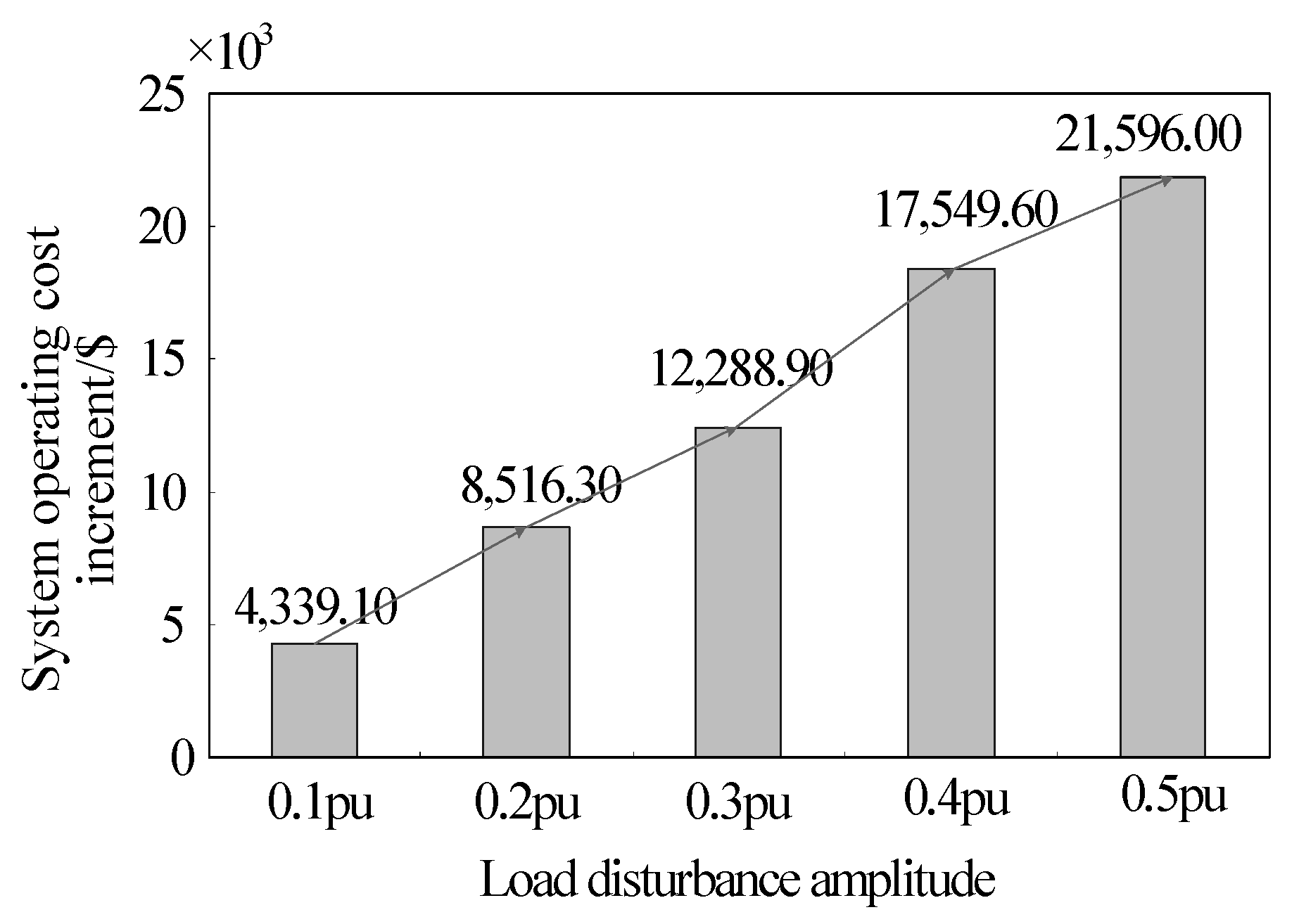
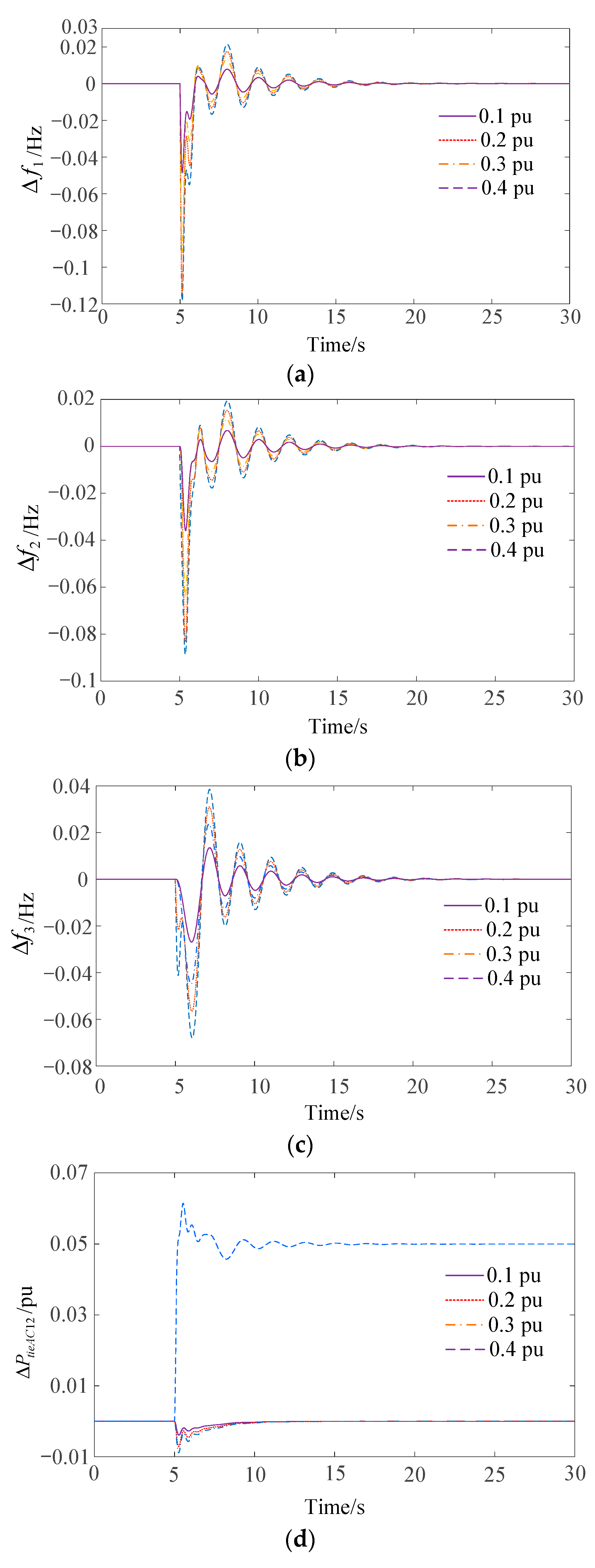
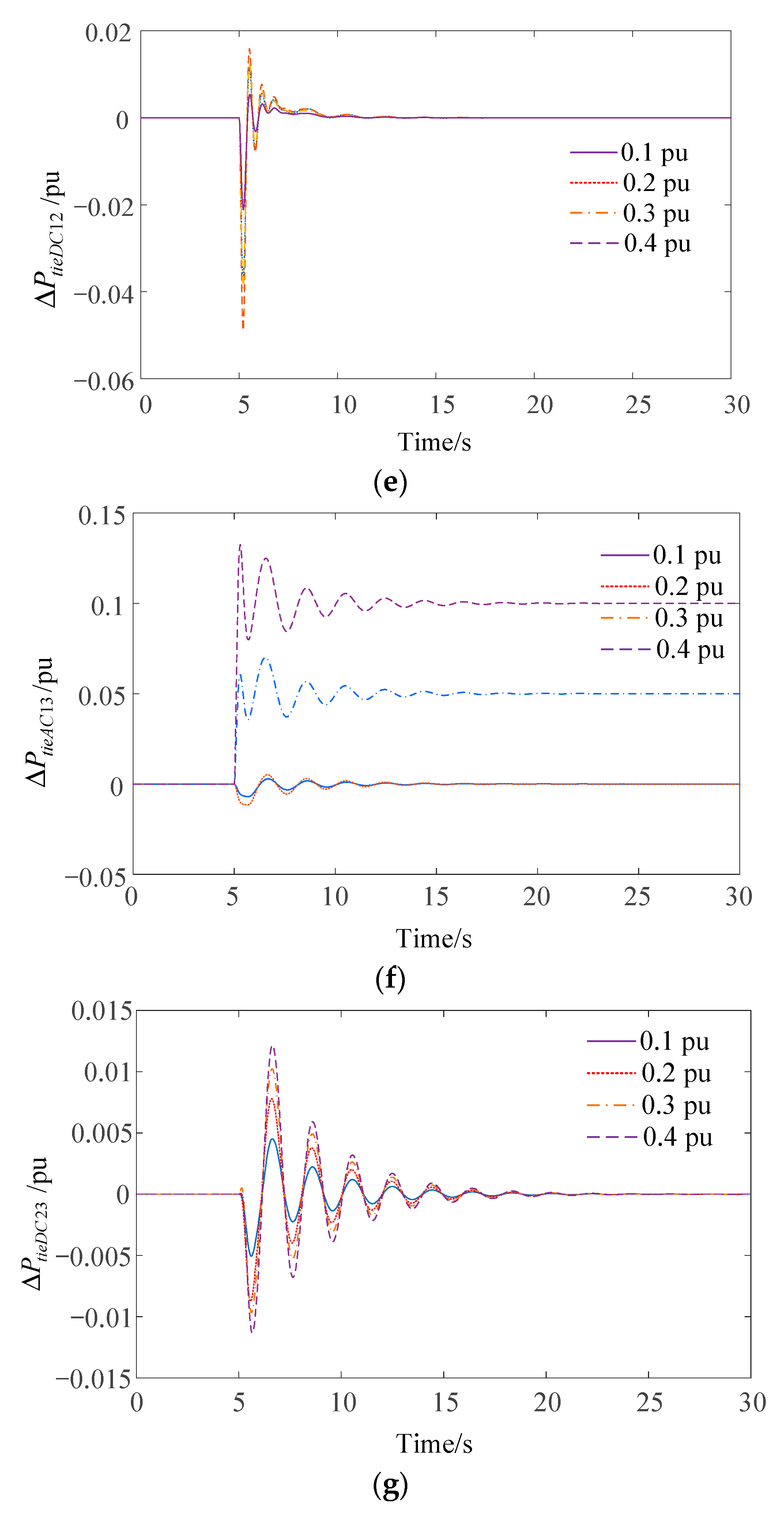
4.1. Case 1: Different Load Step Disturbance

In this scenario, a load step disturbance in Area 1 is set for the power system at t = 5 s simultaneously. The load step disturbance amplitude increases from 0.1 pu to 0.4 pu. The proposed BMPC method can allocate the output of each area AGC unit according to the system operation cost increment optimization principle.

Table 4. Power allocation of AGC units under different load step disturbances.

Load Disturbance Amplitude		0.1 pu	0.2 pu	0.3 pu	0.4 pu
AGC units of Area 1	$P_{G11}$	0.05 pu	0.05 pu	0.05 pu	0.05 pu
	$P_{G12}$	0.0 pu	0.03 pu	0.08 pu	0.08 pu
	$P_{G13}$	0.05 pu	0.12 pu	0.12 pu	0.12 pu
AGC units of Area 2	$P_{G21}$	0.0 pu	0.0 pu	0.0 pu	0.04 pu
	$P_{G22}$	0.0 pu	0.0 pu	0.0 pu	0.01 pu
	$P_{G23}$	0.0 pu	0.0 pu	0.0 pu	0.0 pu
AGC units of Area 3	$P_{G31}$	0.0 pu	0.0 pu	0.0 pu	0.0 pu
	$P_{G32}$	0.0pu	0.0pu	0.05 pu	0.06 pu
	$P_{G33}$	0.0pu	0.0pu	0.0 pu	0.04 pu

gives the steady-state power allocation of AGC units in different regions under different load step disturbances. As seen in Table 4, when the load step disturbance amplitude increases to 0.3 pu, it exceeds the regulation capacity (0.25 pu) of the AGC units in disturbance Area 1, so the AGC units of Area 3 support Area 1’s 0.05 pu through AC tie-line 13. When the load step disturbance amplitude increases to 0.4 pu, the AGC units of Areas 2 and 3 support Area 1’s 0.05 pu and 0.1 pu, respectively. Further, Figure 6 shows the trend of system operating cost increments under different load stepping disturbances. It is easy to see that the system operating cost increment increases linearly with the increased load disturbance amplitude. Also, the increase rate presents an increasing trend. This is due to the increased transmission power of the interarea AC tie-line, which increases its regulation cost.

The dynamic time domain responses of the three-area AC/DC interconnected power system under different load stepping disturbances are shown in Figure 7. It can be seen that the proposed BMPC control method can appropriately control the output of AGC units in three areas according to the total power fluctuation, so the frequency deviations of the three areas are controlled in the range of (−0.12, 0.04) Hz under different load step disturbances. Meanwhile, the DC tie-line power fluctuations between areas are controlled in the safe range. It can also be derived that the BMPC controller stabilizes the load disturbances within about 10 s after the disturbance occurs, which makes frequency deviation maintain around zero, and makes tie-line power fluctuation between areas maintain around default ratings. Due to the limited regulation capacity of the AGC units in Area 1, when the load disturbance amplitude is 0.3 pu and 0.4 pu, the AGC units of Areas 2 and 3 have additional supported power by modifying the AC tie-line transaction protocol. Therefore, the deviation of the AC tie-line is not zero when it restores to steady state, which corresponds to the results in Table 4.

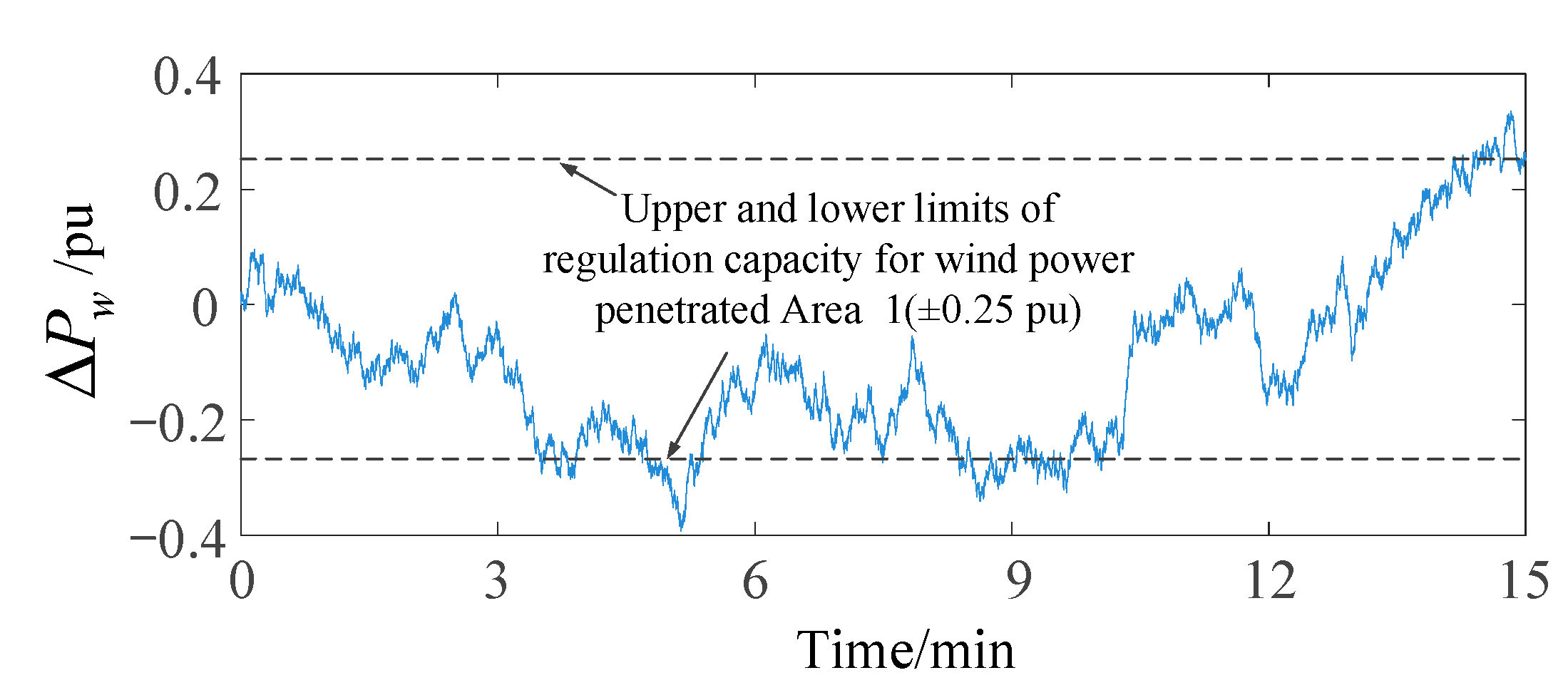
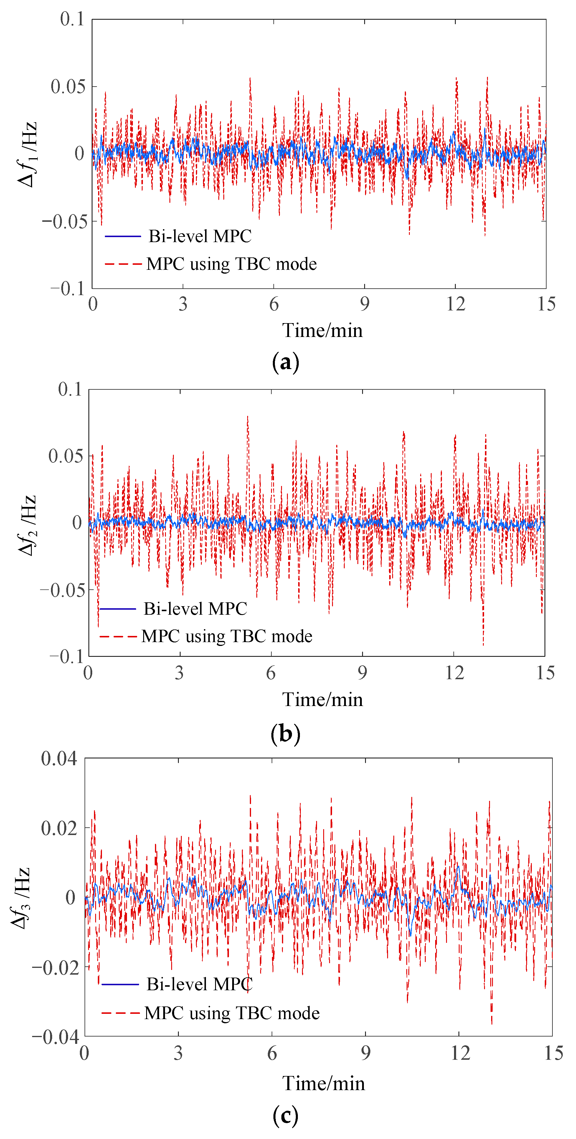
4.2. Case 2: Random Disturbance of Wind Farm

The total capacity of the wind farm in Area 1 is 400 MW, accounting for 20% of the total capacity. It is assumed that the forecast deviation of wind farm output power can be estimated [37], as shown in Figure 8. For comparison, a distributed MPC method in [36] using TBC mode is considered. From the frequency deviation curve of the three-area AC/DC interconnected system shown in Figure 9, the proposed method has better dynamic response performance than the MPC using TBC mode. Compared with the MPC using TBC mode, the frequency deviation of the three-area AC/DC interconnected system always fluctuates around zero using BMPC, and the maximum deviations of the three areas are 0.018, 0.010, and 0.009 Hz. Moreover, when the random disturbance of the wind farm exceeds the lower limit of the regulation capacity of Area 1, the frequency deviation curve of the proposed BMPC control method does not show obvious sharp points around 5 min, but the frequency deviation curve of MPC method using TBC mode shows a sharp rise and sharp point. This also reflects the strong robustness of the proposed BMPC control method. Therefore, the proposed control strategy in this paper can better suppress random disturbances of wind farm output power. Even if it exceeds the regulation capacity of the wind power penetrated area, the proposed control strategy can ensure the frequency stability of AC/DC power grids under large-scale wind farm integration.

Furthermore, the dynamic response performance of the two control methods under random disturbances of wind farm output power is compared in

Table 5. Dynamic response performance comparison of two control methods under output power of wind power random disturbance. TBC, tie-line frequency bias control.

Output	Maximum Deviation		Frequency Root Mean Square Error
	MPC Using TBC Mode	BMPC	MPC Using TBC Mode	BMPC
$\Delta f_1$/Hz	0.057	0.018	0.018	0.005
$\Delta f_2$/Hz	0.079	0.010	0.025	0.003
$\Delta f_3$/Hz	0.029	0.009	0.010	0.003
$\Delta P_{tieAC12}$/pu	0.143	0.048	0.055	0.028
$\Delta P_{tieDC12}$/pu	0.278	0.056	0.042	0.012
$\Delta P_{tieAC13}$/pu	0.219	0.062	0.085	0.020
$\Delta P_{tieAC23}$/pu	0.297	0.093	0.035	0.011
$AC{E}_1$/pu	0.598	0.819	0.035	0.015
$AC{E}_2$/pu	0.405	0.068	0.029	0.010
$AC{E}_3$/pu	0.585	0.039	0.018	0.004

. From the results, the dynamic response performance of BMPC is better than that of MPC using TBC mode. It should be pointed out that the MPC method using TBC mode does not consider the safety of the AC tie-line support. Hence, the maximum deviation of AC tie-lines 12 and 13 in Table 5 exceed the safety limit. In other words, the MPC method using TBC mode cannot provide sufficient regulation capacity to stabilize random fluctuations of wind farm output power, which makes the frequency deviation fluctuation range larger.

The system operating cost increments of the two control methods for random disturbances of a wind farm are given in

Table 6. Economic comparison of two control methods under output power of wind power random disturbance.

Method	System Operating Cost Increment ($)
MPC using TBC mode	19,279.50
BMPC	10,545.30

. The MPC method using TBC mode optimizes the power allocation factor of AGC units every 15 min and remains unchanged during this period. The proposed BMPC method performs rolling optimization of the power allocation factor of AGC units within 5 min at each control domain, which can effectively reduce the regulation cost of multi-area AGC units.

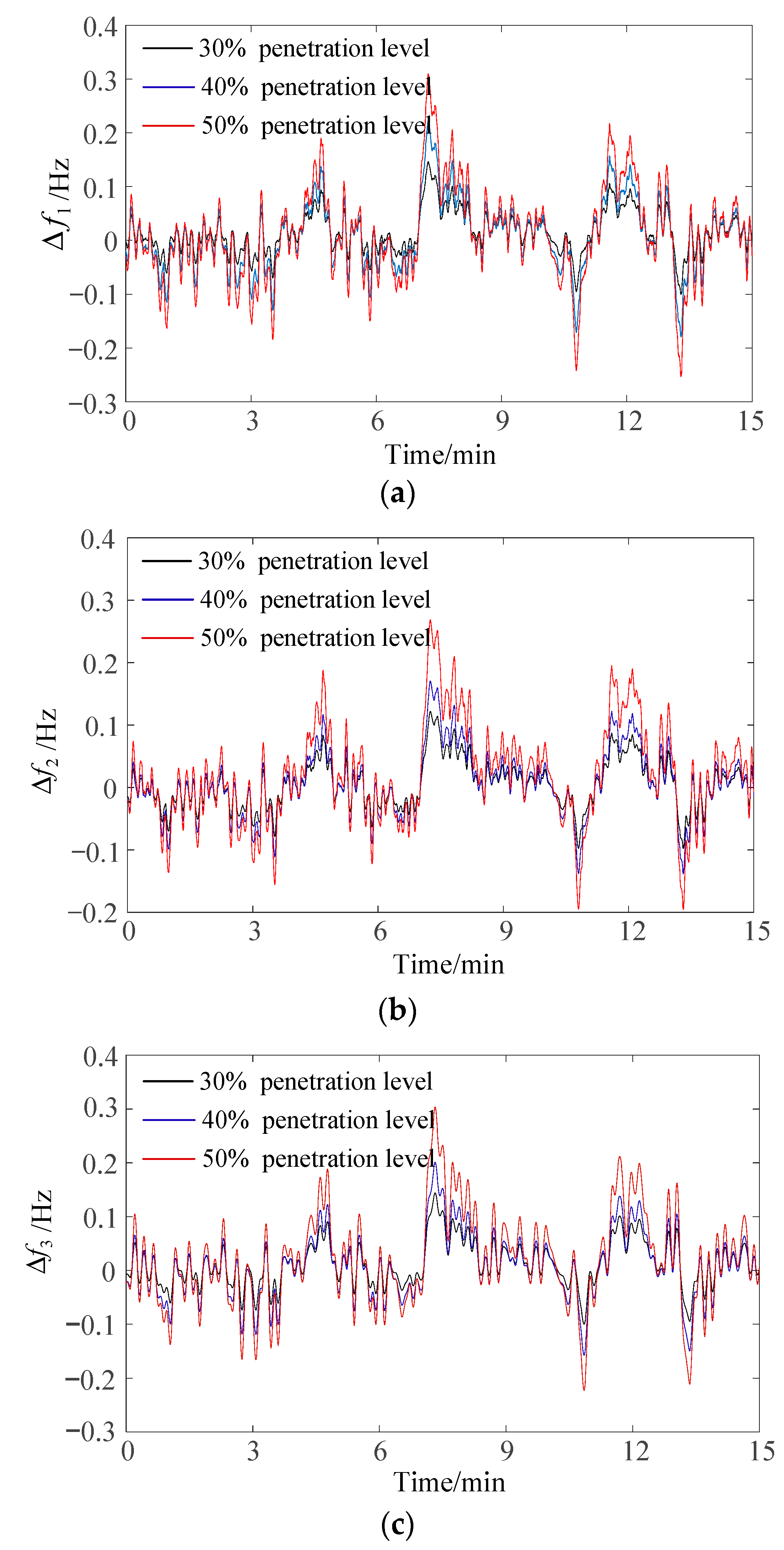
4.3. Case 3: Different Wind Power Penetration

The applicability of the proposed control method under different wind power penetration levels was investigated. The frequency deviation curve of the three-area AC/DC interconnected power grid when the wind power penetration level in Area 1 is 30%, 40%, and 50% is shown in Figure 10. It can be seen that the frequency deviation fluctuation of each area is intensified with increasing wind power penetration. When the wind power penetration level reaches 40%, the proposed method can share the wind power random fluctuation power to every area, so it can still maintain the frequency deviation range of each area within ±0.2 Hz. When the wind power penetration level reaches 50%, the frequency deviation range of each area exceeds the safe range.

5. Conclusions

In order to solve the problem of insufficient frequency regulation capacity of AGC units in wind power penetrated areas, this paper proposes a multi-area AGC unit hierarchical control framework based on bi-level model predictive control. The dynamic simulation results of a three-area AC/DC interconnected power grid with a wind farm show the following:

(1)

Compared with the MPC method using TBC mode [36], the proposed BMPC method not only can keep the frequency deviation within a smaller range under disturbance but also can ensure the safety of AC tie-line power support.

(2)

The proposed BMPC method optimizes the output of AGC units in each area on a minute time scale, avoiding deviation of the AGC unit from the optimal operating point during scheduling periods, which can effectively reduce the frequency regulation cost of multi-area AGC units.

(3)

With increased wind power permeability, the frequency deviation of each regional system fluctuates greatly. When the penetration rate of wind power reaches 40%, the proposed control strategy can still maintain a frequency fluctuation range within ±0.2 Hz, and the wind power random fluctuation power shortage is allocated to maximize the frequency regulation capability of each area.

On the basis of establishing a detailed AGC model of a wind farm and incorporating it into economic frequency control of multi-area AGC units, it can not only improve the dispatchability of the wind farm, but also improve the economy of the AGC units. Therefore, the coordinated control of multi-area AGC units considering a detailed wind farm model needs to be further studied. In addition, a real object experiment is too complicated to realize in our current experimental conditions.

References

1. Fox, B. Introduction. In Wind Power Integration: Connection and System Operational Aspects; IET Power and Energy Series; Institution of Engineering and Technology: Stevenage, UK, 2007; Volume 50, pp. 77–85. [Google Scholar]
2. Suh, J.; Yoon, D.H.; Cho, Y.S.; Jang, G. Flexible frequency operation strategy of power system with high renewable penetration. IEEE Trans. Sustain. Energy 2017, 8, 192–199. [Google Scholar] [CrossRef]
3. Keyhani, A.; Chatterjee, A. Automatic generation control structure for smart power grids. IEEE Trans. Smart Grid 2012, 3, 1310–1316. [Google Scholar] [CrossRef]
4. Zhang, L.; Luo, Y.; Ye, J.; Xiao, Y.-Y. Distributed coordination regulation marginal cost control strategy for automatic generation control of interconnected power system. IET Gener. Transm. Distrib. 2017, 11, 1337–1344. [Google Scholar] [CrossRef]
5. Bevrani, H. Robust Power System Frequency Control, 2nd ed.; Springer: Gewerbestrasse, Switzerland, 2014. [Google Scholar]
6. Chen, C.; Zhang, K.; Yuan, K.; Gao, Z.; Teng, X.; Ding, Q. Disturbance rejection-based LFC for multi-area parallel interconnected AC/DC system. IET Gener. Transm. Distrib. 2016, 10, 4105–4117. [Google Scholar] [CrossRef]
7. Patel, R.B.; Li, C.; Yu, X.; McGrath, B. Optimal automatic generation control of an interconnected power system under network constraints. IEEE Trans. Ind. Electron. 2018, 65, 7220–7228. [Google Scholar] [CrossRef]
8. Sahu, R.K.; Panda, S.; Chandra Sekhar, G.T. A novel hybrid PSO-PS optimized fuzzy PI controller for AGC in multi area interconnected power systems. Int. J. Electr. Power Energy Syst. 2015, 64, 880–893. [Google Scholar] [CrossRef]
9. Raju, M.; Saikia, L.C.; Sinha, N. Automatic generation control of a multi-area system using ant lion optimizer algorithm based PID plus second order derivative controller. Int. J. Electr. Power Energy Syst. 2016, 80, 52–63. [Google Scholar] [CrossRef]
10. Arya, Y. AGC performance enrichment of multi-source hydrothermal gas power systems using new optimized FOFPID controller and redox flow batteries. Energy 2017, 127, 704–715. [Google Scholar] [CrossRef]
11. Sharma, Y.; Saikia, L.C. Automatic generation control of a multi-area ST—Thermal power system using Grey Wolf Optimizer algorithm based classical controllers. Int. J. Electr. Power Energy Syst. 2015, 73, 853–862. [Google Scholar] [CrossRef]
12. Camacho, E.F.; Bordons, C. Model Predictive Control; Springer: London, UK, 2004; Volume 2. [Google Scholar]
13. Mayne, D. Model predictive control: Recent developments and future promise. Automatica 2014, 50, 2967–2986. [Google Scholar] [CrossRef]
14. Wang, L. Model Predictive Control System Design and Implementation Using MATLAB; Springer: London, UK, 2009. [Google Scholar]
15. Ersdal, A.M.; Imsland, L.; Uhlen, K. Model predictive load-frequency control. IEEE Trans. Power Syst. 2015, 31, 777–785. [Google Scholar] [CrossRef]
16. Mohamed, T.H.; Morel, J.; Bevrani, H.; Hiyama, T. Model predictive based load frequency control design concerning wind turbines. Int. J. Electr. Power Energy Syst. 2012, 43, 859–867. [Google Scholar] [CrossRef]
17. Elsisi, M.; Soliman, M.; Aboelela, M.; Mansour, W. Bat inspired algorithm based optimal design of model predictive load frequency control. Int. J. Electr. Power Energy Syst. 2016, 83, 426–433. [Google Scholar] [CrossRef]
18. Zheng, Y.; Li, S.; Qiu, H. Networked coordination-based distributed model predictive control for large-scale system. IEEE Trans. Control Syst. Technol. 2013, 21, 991–998. [Google Scholar] [CrossRef]
19. Venkat, A.N.; Hiskens, I.A.; Rawlings, J.B.; Wright, S.J. Distributed MPC strategies with application to power system automatic generation control. IEEE Trans. Control Syst. Technol. 2008, 16, 1192–1206. [Google Scholar] [CrossRef]
20. Ma, M.; Chen, H.; Liu, X.; Allgöwer, F. Distributed model predictive load frequency control of multi-area interconnected power system. Int. J. Electr. Power Energy Syst. 2014, 62, 289–298. [Google Scholar] [CrossRef]
21. Liu, X.; Kong, X.; Lee, K.Y. Distributed model predictive control for load frequency control with dynamic fuzzy valve position modelling for hydro–thermal power system. IET Control. Theory Appl. 2016, 10, 1653–1664. [Google Scholar] [CrossRef]
22. Zheng, Y.; Zhou, J.; Xu, Y.; Zhang, Y.; Qian, Z. A distributed model predictive control based load frequency control scheme for multi-area interconnected power system using discrete-time Laguerre functions. ISA Trans. 2017, 68, 127–140. [Google Scholar] [CrossRef]
23. Ma, M.; Liu, X.; Zhang, C. LFC for multi-area interconnected power system concerning wind turbines based on DMPC. IET Gener. Transm. Distrib. 2017, 11, 2689–2696. [Google Scholar] [CrossRef]
24. Liu, X.; Zhang, Y.; Lee, K.Y. Coordinated distributed MPC for load frequency control of power system with wind farms. IEEE Trans. Ind. Electron. 2017, 64, 5140–5150. [Google Scholar] [CrossRef]
25. Christofides, P.D.; Scattolini, R.; de la Peña, D.M.; Liu, J. Distributed model predictive control: A tutorial review and future research directions. Comput. Chem. Eng. 2013, 51, 21–41. [Google Scholar] [CrossRef]
26. Picasso, B.; De Vito, D.; Scattolini, R.; Colaneri, P. An MPC approach to the design of two-layer hierarchical control systems. Autom. 2010, 46, 823–831. [Google Scholar] [CrossRef]
27. Zhang, T.; Gooi, H.B. Hierarchical MPC-based energy management and frequency regulation participation of a virtual power plant. In Proceedings of the IEEE Innovative Smart Grid Technologies Conference Europe, Istanbul, Turkey, 12–15 October 2014. [Google Scholar]
28. Babahajiani, P.; Shafiee, Q.; Bevrani, H. Intelligent Demand Response Contribution in Frequency Control of Multi-Area Power Systems. IEEE Trans. Smart Grid 2018, 9, 1282–1291. [Google Scholar] [CrossRef]
29. Sharma, G.; Nasiruddin, I.; Niazi, K.R.; Bansal, R.C. Robust automatic generation control regulators for a two-area power system interconnected via AC/DC tie-lines considering new structures of matrix Q. IET Gener. Transm. Distrib. 2016, 10, 3570–3579. [Google Scholar] [CrossRef]
30. Niazi, K.R.; Bansal, R.C.; Sharma, G.; Nasiruddin, I. Optimal AGC of a multi-area power system with parallel AC/DC tie lines using output vector feedback control strategy. Int. J. Electr. Power Energy Syst. 2016, 81, 22–31. [Google Scholar]
31. Scattolini, R. Architectures for distributed and hierarchical model predictive control–A review. J. Process Control 2009, 19, 723–731. [Google Scholar] [CrossRef]
32. Mohamed, T.H.; Bevrani, H.; Hassan, A.A.; Hiyama, T. Decentralized model predictive based load frequency control in an interconnected power system. Energy Convers. Manag. 2011, 52, 1208–1214. [Google Scholar] [CrossRef]
33. Mohamed, T.H.; Morel, J.; Bevrani, H.; Hassan, A.A.; Mohamed, Y.S.; Hiyama, T. Decentralized model predictive-based load-frequency control in an interconnected power system concerning wind turbines. IEEJ Trans. Electr. Electron. Eng. 2012, 7, 487–494. [Google Scholar] [CrossRef]
34. Kennel, F.; Gorges, D.; Liu, S. Energy management for smart grids with electric vehicles based on hierarchical MPC. IEEE Trans. Ind. Inf. 2013, 9, 1528–1537. [Google Scholar] [CrossRef]
35. Ma, M.; Zhang, C.; Liu, X.; Chen, H. distributed model predictive load frequency control of the multi-area power system after deregulation. IEEE Trans. Ind. Electron. 2017, 64, 5129–5139. [Google Scholar] [CrossRef]
36. Liao, X.; Liu, K.; Wang, N.; Liang, Q.; Ma, Y.; Chen, Z.; Ding, K.; Zhou, Q. Cooperative DMPC-based load frequency control of AC/DC interconnected power system with solar thermal power plant. In Proceedings of the 2018 IEEE PES Asia-Pacific Power and Energy Engineering Conference (APPEEC), Kota Kinabalu, Sabah, Malaysia, 7–10 October 2018; pp. 341–346. [Google Scholar]
37. Zhang, Y.; Liu, K.; Qin, L.; An, X. Deterministic and probabilistic interval prediction for short-term wind power generation based on variational mode decomposition and machine learning methods. Energy Convers. Manag. 2016, 112, 208–219. [Google Scholar] [CrossRef]
Figure 1. Diagram of automatic generation control (AGC) model for control area i with wind farm. ACE, area control error.
Processes 07 00669 g001
Figure 2. General structure of model predictive control (MPC) scheme.
Processes 07 00669 g002
Figure 3. Bi-level model predictive control framework. EMPC, upper-level economic model predictive control; DMPC, distributed model predictive control.
Processes 07 00669 g003
Figure 4. Coordinated control scheme for AGC units with wind farm across control areas.
Processes 07 00669 g004
Figure 5. Three-area AC/DC interconnected power grid with wind farm.
Processes 07 00669 g005
Figure 6. System operating cost increments under different load stepping disturbances.
Processes 07 00669 g006
Figure 7. Dynamic time domain responses of three-area system under different load stepping disturbances: (a) frequency deviation of Area 1; (b) frequency deviation of Area 2; (c) frequency deviation of Area 3; (d) power deviation of AC tie-line 12; (e) power deviation of DC tie-line 12; (f) power deviation of AC tie-line 13; (g) power deviation of AC tie-line 23.
Processes 07 00669 g007aProcesses 07 00669 g007b
Figure 8. Forecast deviation of wind farm output power.
Processes 07 00669 g008
Figure 9. Frequency deviation of three-area system under output power of wind power random disturbance: (a) Area 1; (b) Area 2; (c) Area 3.
Processes 07 00669 g009
Figure 10. Frequency deviation of three-area system under different wind power penetration: (a) Area 1; (b) Area 2; (c) Area 3.
Processes 07 00669 g010