Pore Structure Prediction from Well Logs in Deep Tight Sandstone Reservoirs Using Machine Learning Methods

Abstract

In this study, deep tight sandstone was selected as an example to propose a complete method for predicting reservoir pore structure by capillary pressure curves and conventional well log data. This method pioneers the integration of grey relational analysis, principal component analysis, ensemble clustering, and deep neural networks to establish a systematic predictive framework for transitioning from conventional logging data to pore structure types. A total of 186 core data from three wells were used in this study. First, sensitive pore structure parameters from mercury injection capillary pressure data were extracted using grey correlation analysis and principal component analysis. Then, unsupervised clustering analysis was applied to classify the reservoir pore structures in the study area, dividing it into three categories. These category labels were combined with conventional well logs to create learning samples for a deep neural network (DNN) model developed to predict reservoir pore structure categories. The accuracy of the training set of the model reached 88.2%, while the accuracy of the testing set was 80.43%. Finally, the method was applied to field well log data. The results showed significant differences in pore structure classifications among gas layers, water–gas layers, and dry layers. This method is versatile, with its core components transferable to other deep sandstone reservoir studies, and can accurately predict the pore structure of tight sandstone reservoirs, which is critical for advancing the characterization of deep and complex oil and gas reservoirs.

1. Introduction

Deep and ultra-deep formations have become strategic areas for securing China’s oil and gas supply and optimizing its energy structure. In the Kuqa Depression of the Tarim Basin, multiple gas fields have been discovered, including Keshen, Bozi, Dabei, Kela, and Dina. The deep and ultra-deep continental oil and gas systems in this region hold resources equivalent to 5.05 × 10⁹ tons of oil, with proven reserves of 1.38 × 10⁹ tons [1]. This study focuses on deep tight sandstones in this region, with core research value and significance centered on two aspects including reservoir characteristics and resource attributes. From a reservoir perspective, these deep tight sandstone reservoirs are influenced by structural factors, diagenesis, and compaction. They typically exhibit low porosity and permeability, with complex micrometer- and submicron-scale pore throats. This pore structure not only governs hydrocarbon migration and accumulation but also determines hydrocarbon flow characteristics. Precise assessment of pore structure plays a vital role in predicting how hydrocarbons are distributed and migrate, as well as assessing reservoir performance. From a reserve and hydrocarbon accumulation perspective, deep hydrocarbon reserves are primarily hosted within tight sandstones, whose physical properties dictate reserve scale and enrichment intensity.

Pore structures are characterized by the quantity, size, geometry, distribution, and connectivity of pores and throats [2,3]. Common evaluation methods include mercury intrusion capillary pressure (MICP), scanning electron microscopy (SEM), nuclear magnetic resonance (NMR), X-ray computed tomography (XCT), infrared spectroscopy (AFM-IR), and gas adsorption [4,5,6]. Specifically, MICP reveals pore-throat size and connectivity [7]; SEM provides pore morphology [8]; NMR analyzes multifractal characteristics of the T₂ relaxation spectrum [9,10]; XCT enables nanoscale 3D visualization [11,12,13]; and gas adsorption quantifies pore characteristics through gas uptake at varying relative pressures [14]. Although laboratory techniques provide detailed pore structure parameters, they are limited to core samples and cannot feasibly be applied to every well or depth.

Traditionally, pore structure parameters are estimated from well log data by building predictive models based on laboratory measurements. These models are developed using conventional or NMR logging data through algorithms such as multiple regression. Early studies predominantly employed this multivariate regression approach combining conventional logging data with core experimental results. With advancements in microscale experimental techniques, subsequent research has progressively integrated multiscale microscopic experimental methods including X-ray diffraction (XRD), MICP, and SEM with NMR logging technology. This integration has enabled a leap in reservoir pore structure characterization from macroscopic statistics to microscopic quantification. Simultaneously, the parameters used to characterize pore structure have expanded beyond macroscopic physical properties like porosity and permeability to include microscopic pore structure parameters such as the displacement pressure, sorting coefficient, and structural coefficient. This provides a more reliable basis for precise reservoir classification and quantitative parameter prediction [15,16,17,18,19,20,21]. However, the accuracy of these methods is limited, and NMR logging has not been widely applied across all regions, especially in deep and ultra-deep formations where data acquisition is particularly challenging. Consequently, machine learning methods have been introduced to integrate core data with conventional logs for improved pore structure characterization. Machine learning enables the identification of complex patterns and correlations for accurate prediction and classification of reservoir parameters. In this study, it is first used to classify core data through unsupervised learning methods such as K-Means clustering [22,23], hierarchical clustering [24], second-order clustering [25,26,27], decision trees [28], and self-organizing maps (SOMs) [29]. Clustering validity is assessed using Bayes discriminant analysis [26]. Machine learning also enables modeling of nonlinear relationships between well logs and core-derived parameters, supporting accurate prediction and classification. Neural networks, a core technique in machine and deep learning, have been widely used to evaluate complex pore structures from logging, testing, and geological data, allowing continuous reservoir classification [30,31,32,33,34]. For example, Liao et al. (2020) combined core MICP clustering with a two-layer convolutional neural network to predict pore categories from logs [35]. Han (2021) applied support vector machines (SVMs) to classify non-core intervals based on capillary pressure and logs, aligning well with core data [36]. The LightGBM algorithm outperformed other neural networks for reservoir classification, as reported by Yang et al. (2025) [37]. Decision trees, k-nearest neighbors, and SVMs have also been used to identify ultra-low-permeability reservoirs [38]. Genetic algorithm-optimized neural networks have predicted permeability and classified lithology using parameters such as the pore aspect ratio and shear factor [39]. The Random Forest model was applied to quantify the relationship between paraffin content and production performance [40]. Image-based models, including backpropagation neural networks (BPNs) and stacked autoencoders (SAEs), have been applied to classify porosity from thin-section images [41]. Probabilistic neural networks and boosted regression models have been used to predict permeability [42]. Although existing research has made progress in utilizing clustering and deep learning (DNN) for reservoir characterization, most approaches perform clustering classification independently and then directly apply the clustering results to DNN training. Furthermore, clustering input parameters are not screened, making the results prone to deviation from geological reality due to parameter redundancy and multicollinearity. Furthermore, the model’s generalization capability is constrained by the random errors inherent in a single clustering method, making it difficult to ensure stability and reliability. Although numerous methods exist for evaluating and predicting pore structure using laboratory and logging data, a systematic procedure remains lacking.

Therefore, this study focuses on deep tight sandstone reservoirs and proposes an integrated workflow for predicting pore structure based on capillary pressure curves and conventional well logs. The pore structure parameters are initially extracted from the capillary pressure data and subsequently analyzed using grey relational analysis and principal component analysis to screen characteristic parameters and eliminate multicollinearity effects. Based on these results, a voting-based clustering method is employed to classify rock core samples, thereby reducing the error associated with a single clustering algorithm. Finally, the classification results and logging data are used to train a neural network model for predicting the pore structure characteristics of the entire reservoir.

2. Materials, Study Area, and Data

Situated on the northern margin of the Tarim Basin, the Kuqa Depression is a foreland basin formed on a Paleozoic folded basement. Under the influence of the tectonic activity in the southern Tianshan orogenic belt, the region generally slopes from high elevations in the north to lower elevations in the south. Seven structural belts with nearly east–west strikes are developed from north to south. Figure 1a shows the regional tectonic map, while Figure 1b depicts the geographical location of the region; the Dibei gas reservoir is positioned at the central part of the Dibei slope zone. The target reservoir is the Lower Jurassic Ahe Formation, which comprises interbedded sandstone and mudstone (J1a1), upper conglomerate (J1a2), and lower conglomerate (J1a3) from top to bottom. The Ahe Formation is primarily characterized by braided river delta plain subfacies deposition, characterized by low compositional maturity, which makes it difficult to classify the pore structure, and the data in this study were collected from this stratigraphic section. The lithology predominantly consists of gravel-bearing coarse sandstone and medium sandstone, with sand bodies that crisscross and overlap. The reservoir has a thickness ranging from 260 to 300 m [43].

The natural gas distribution in the Dibei gas reservoir is complex. It exhibits characteristics similar to tight sandstone gas reservoirs of the trap type, being mainly distributed within structural traps. At the same time, it also shares features with continuous tight sandstone gas reservoirs that are not entirely controlled by structural factors. As a result, it represents a transitional type of gas reservoir between these two end-members [43,44,45]. The overlying Jurassic Yangxia Formation contains thick sequences of coal seams and dark mudstone, while the underlying Triassic Taliqike Formation likewise develops substantial dark mudstone. These two formations have significant thickness and high organic matter abundance, functioning as both source rocks and effective cap rocks. They overlap with the Jurassic Ahe Formation reservoir in a “sandwich” configuration, forming an optimal source–reservoir–seal assemblage. The close spatial association between source rocks and reservoirs improves hydrocarbon generation, expulsion, and accumulation efficiency, making it a key factor in tight sandstone gas formation and reservoir development in the Dibei region [44].

Figure 1. Structural position of the Dibei gas reservoirs. (a) Regional tectonic map of the Dibei gas reservoir; (b) Geographical location of the Dibei gas reservoir. (modified after Li et al. 2025 [46]).

Figure 1. Structural position of the Dibei gas reservoirs. (a) Regional tectonic map of the Dibei gas reservoir; (b) Geographical location of the Dibei gas reservoir. (modified after Li et al. 2025 [46]).

In this study, three wells (YN2C, YN4, and YN5) in the Dibei area are used. The well logs in the three wells contain Caliper (CAL), Gamma Ray (GR), Bulk Density (DEN), Neutron Porosity (CNL), and Acoustic Transit Time (DT). The resistivity of the three wells are array induction logs or dual induction logs, including deep induction and medium induction logs.

A total of 186 samples from the target formation in the three wells were chosen, cut, and ground into regular blocks. These 186 samples encompass multiple reservoir types, including oil-bearing layers, residual oil layers, water–oil-bearing layers, and dry layers. These samples were first subjected to oil and salt washing. Then, the porosity and permeability were measured using the helium method via a helium porosimeter. Next, after vacuum drying to remove moisture and impurities within pores, the helium displacement method was employed to determine the true volume of the solid rocks. The mercury intrusion process in large pores was measured using a low-pressure system, followed by high-pressure system measurements for small-pore filling data. Original data were recorded at each pressure point after stabilization.

In the reservoir classification prediction model with DNN, the GR, DEN, CNL, DT, deep resistivity (M2RX or RD), and shallow resistivity (M2R3 or RM) are used. The six logs reflect the properties of lithology, the physical properties, and the oiliness of the reservoir. After importing core data into the software, the core depth is repositioned by comparing the porosity values of the cores with the density logs, so that the trend of the core porosity after repositioning is consistent with the density log curves. Then, the curve values corresponding to the depth of each sample were extracted. In total, 75 percent of core samples with the corresponding log values were selected as the training set, with the test set comprising the remaining 25 percent of samples. During partitioning, 138 samples are randomly selected from the dataset as the training set, followed by randomly selecting the remaining data as the validation set.

3. Methods

3.1. Pore Structure Parameters Based on MICP Curve

The capillary pressure curve illustrates the relationship between pressure and pore-throat radius, revealing the distribution of pore throats within rocks. Typically derived from MICP tests, these curves help characterize the pore-throat ratio, sorting, flow properties, uniformity, and connectivity [47,48]. The key pore structure parameters used in this study are as follows:

(1)

Displacement pressure (P_d): Capillary pressure at the largest connected pore throat, identified as the inflection point on mercury injection curves with clear linear segments.

(2)

Maximum connected pore-throat radius (R_d): The radius of the largest interconnected pore throat that permits the non-wetting phase to first enter the rock matrix. The expression is as follows [49]:

$$R_d={\displaystyle \frac{2\gamma \cos \theta }{P_d}},$$

(1)

where $\gamma$ represents the surface tension of mercury, and $\theta$ denotes the angle of contact. According to generally accepted standards in the field of rock physics, the surface tension of mercury is taken as 485 mN/m, and the angle of contact is taken as 140°.

(3)

Median pressure (P₅₀): Capillary pressure at 50% mercury saturation on the capillary pressure curve. It can be further converted to median aperture through a capillary pressure equation.

(4)

Median pore-throat radius (R₅₀): Pore-throat radius at 50% mercury saturation, which represents the median size of interconnected flow channels in the rock. The expression is as follows [21]:

$$R_{50}={\displaystyle \frac{2\gamma \cos \theta }{P_{50}}},$$

(2)

(5)

Sorting coefficient (S_p): Quantitative indicator of pore size distribution uniformity in reservoir rocks, with higher values signifying greater heterogeneity in pore-throat sizes. The expression of S_p is as follows [50]:

$$S_p={\displaystyle \frac{R_{84}-R_{16}}{4}}+{\displaystyle \frac{R_{95}-R_5}{6.6}},$$

(3)

where R_i represents the pore radius at a cumulative saturation of i%, which can be calculated by expressions similar to Equations (1) and (2).

(6)

Relative sorting coefficient (D): This is a normalized metric that quantifies pore size heterogeneity by measuring deviations from R₅₀ relative to the standard sorting coefficient. A smaller D value indicates better throat sorting and weaker reservoir heterogeneity. This not only governs the absolute permeability of the rock but also fundamentally influences the fluid flow patterns during water injection development and ultimately affects the recovery rate. The expression of D is as follows [51]:

$$D=S_p/D_m,$$

(4)

where D_m represents average pore radius.

(7)

Structural coefficient (J): Dimensionless parameter that quantifies interphase interactions in multiphase flow, reflecting the mutual influence and coupling between fluid phases within porous media. The expression of structural coefficient is as follows [52]:

$$J={\displaystyle \frac{\overline{R^2}\varphi }{8K}},$$

(5)

where $\varphi$ represents the porosity (dimensionless, expressed as a decimal value between 0 and 1), $\overline{R}$ denotes the mean pore-throat radius (micrometers, μm), and K represents the permeability (millidarcies, mD).

(8)

Characteristic structural coefficient (Ch): A dimensionless parameter that quantifies the wettability-controlled flow capacity in multiphase systems, reflecting how the internal pore structure of the rock influences fluid-phase interactions. Its value is closely related to permeability. Research data indicates that the Ch of medium-to-high-permeability reservoirs increases with increasing permeability. The expression of this parameter is as follows [52]:

$$Ch={\displaystyle \frac{1}{DJ}},$$

(6)

where D is the relative sorting coefficient and J is the structural coefficient.

(9)

Homogeneity coefficient (α): The homogeneity coefficient represents the average-to-maximum pore diameter ratio, characterizing the deviation degree of individual pore-throat radii relative to the maximum pore-throat radius in porous media. Its calculation equation is as follows [53]:

$$\alpha ={\displaystyle \frac{\overline{R}}{R_{\max }}},$$

(7)

where $R_{\max }$ represents the maximum pore-throat radius (micrometers, μm).

(10)

Pore-throat skewness (S_kp): A statistical parameter that characterizes the asymmetry of the pore-throat size distribution, indicating whether smaller or larger pore-throat radii dominate within the rock fabric. It can also be regarded as a measure of the modal concentration of pore-throat sizes. The expression of pore-throat skewness is given as follows [54]:

$$S_{kp}={\displaystyle \frac{R_{84}+R_{16}-2R_{50}}{2\left(R_{84}-R_{16}\right)}}+{\displaystyle \frac{R_{95}+R_5-2R_{50}}{2\left(R_{95}-R_5\right)}}.$$

(8)

3.2. Classification of Pore Structure of Core Samples

There are many parameters derived from MICP curves, making it complex to classify the pore structures of core samples. Therefore, these parameters underwent standardized preprocessing before being incorporated into subsequent analytical workflows. In this study, parameters that more effectively reflect pore structure characteristics were first selected. Principal component analysis (PCA) was then utilized to perform dimensionality reduction on the selected parameters. Finally, the rock samples were classified using multiple clustering analysis methods, and the final classification was determined through a voting-based ensemble approach.

3.2.1. Selection of Pore Structural Parameters

The capillary pressure curve allows for the calculation of numerous pore structure parameters, each reflecting different aspects of pore structure characterization. In this study, grey relational analysis is employed to identify the parameters most strongly correlated with pore structure for subsequent classification. The Flow Zone Indicator (FZI), which is widely used to characterize reservoir flow capacity, demonstrates a high degree of correlation with pore structure because it is directly related to porosity and permeability [55]. Compared to single permeability parameters, the Rock Quality Index (RQI), and nuclear magnetic resonance (NMR)-derived parameters, the FZI is chosen as the index parameter for pore structure screening. Based on the modified Kozeny–Carmen equation, the FZI is a parameter extracted from permeability and porosity that directly characterizes the essence of microscopic pore structure, enabling effective differentiation between reservoir types with distinct flow characteristics. In contrast, the single permeability parameter only provides a macroscopic reflection of reservoir fluid flow capacity and cannot distinguish the fundamental differences between various pore structure types. While the RQI establishes a correlation between permeability and porosity, it fails to account for the impact of bound water saturation on effective flow pores, making it difficult to eliminate interference from micro-pores in tight sandstones. NMR-derived parameters can intuitively reflect pore size distribution, but face limitations in deep and ultra-deep formations. High-temperature and high-pressure logging environments affect the applicability of NMR instruments, and data acquisition costs are high. In comparison, FZI calculations rely solely on conventional logging data or core test results which are readily available and cost-effective, and the FZI is more suitable as an indicator parameter for selecting pore structures in highly heterogeneous tight sandstone reservoirs. The expression of this parameter is as follows [56,57]:

$$RQI=0.0314\sqrt{{\displaystyle \frac{K}{\varphi }}}.$$

(9)

$$FZI=RQI{\displaystyle \frac{1-\varphi }{\varphi }}.$$

(10)

where $\varphi$ denotes the porosity (%), and K represents the permeability (mD).

Grey relational analysis is a multivariate statistical method for assessing similarity between datasets, used to evaluate correlations among pore structure parameters [58]. The grey relational coefficient (ξ_i(k)) between the normalized reference and comparative sequences is expressed as follows [59]:

$${\xi }_i\left(k\right)={\displaystyle \frac{\underset{i}{\min } \underset{k}{\min }\left|y\left(k\right)-x_i\left(k\right)\right|+p \underset{i}{\max } \underset{k}{\max }\left|y\left(k\right)-x_i\left(k\right)\right|}{\left|y\left(k\right)-x_i\left(k\right)\right|+p \underset{i}{\max } \underset{k}{\max }\left|y\left(k\right)-x_i\left(k\right)\right|}}.$$

(11)

$$r_i={\displaystyle \frac{1}{n}}{\displaystyle \sum _{k=1}^n{\xi }_i\left(k\right),k=1,2,\dots ,n}$$

(12)

where x denotes the comparative sequence, m represents the number of comparative sequences, y indicates the normalized reference sequence, ξ_i(k) stands for the grey relational coefficient, and p presents the distinguishing coefficient (0–1), typically set to 0.5. Setting the distinguishing coefficient to 0.5 balances noise interference and sensitivity to variation, though it may reduce resolution when data exhibits significant fluctuations. In this study, the PCA-processed data exhibited minimal variability, rendering the 0.5 coefficient appropriate.

3.2.2. Principal Component-Based Dimensionality Reduction Analysis

The pore structure parameters exhibit multicollinearity issues, which may compromise the accuracy of subsequent classification. PCA can effectively address multicollinearity in multidimensional data by transforming the data into eigenvectors. Then, the principal components are screened based on the contribution rates of their corresponding eigenvalues, thereby achieving the goal of reducing multicollinearity [60,61,62]. The principal component analysis algorithm is a linear method, which has limitations in dealing with complex nonlinear data. Although nonlinear dimensionality reduction methods such as t-distributed Stochastic Neighbor Embedding (t-SNE) and autoencoders can theoretically capture the nonlinear structure of data, they exhibit the following limitations in practical applications that render them unsuitable for this study: The t-SNE algorithm is sensitive to hyperparameters and exhibits randomness in its computational results, making it difficult to provide stable features for subsequent pore structure analysis. Autoencoders typically require large-scale labeled data for thorough training, whereas this study has a limited number of available core samples, making them prone to overfitting under small-sample conditions. In contrast, although PCA has its limitations, its computational simplicity and strong interpretability of results make it more suitable for the core requirements of this study. In this paper, PCA was performed on the screened pore structure parameters to construct synthetic pore structure parameters that retain the essential information of the original variables while demonstrating low multicollinearity.

Principal component analysis is used to calculate the covariance matrix of normalized data. Thereafter, the covariance matrix is then subjected to eigenvalue decomposition, yielding both eigenvalues and their respective eigenvectors. The calculation formula is as follows [61]:

$$C={\displaystyle \frac{1}{n-1}}X{\prime }^{T}X\prime .$$

(13)

$$Cv=\lambda v.$$

(14)

where X′ represents the normalized standard matrix, λ denotes the eigenvalue, v is the corresponding eigenvector, and C stands for the covariance matrix. The eigenvalues and eigenvectors can quantify the contribution of different data features. A larger eigenvalue indicates that the corresponding eigenvector contains more significant information.

3.2.3. Classification of Pore Structure by Unsupervised Learning Methods

Unsupervised learning clustering algorithms are data analysis methods that partition datasets into multiple clusters based on the similarity between data points. In the case of no reliance on manual annotation, unsupervised learning technology can directly conduct independent analysis based on unmarked datasets, effectively overcoming the actual limitation of scarce data annotation resources, and is suitable for practical application scenarios with scarce labels. Among these approaches, three methods have demonstrated particularly effective performance: K-Means, Fuzzy C-Means (FCM), and the Gaussian Mixture Model (GMM). K-Means, FCM, and the GMM, respectively, provide hard-cutting cluster centers, fuzzy membership functions, and probabilistic models, forming a complementary classification system. Given that the data in this study exhibits dispersed characteristics and lacks typical density features after PCA dimensionality reduction, these three methods were selected.

The K-Means algorithm begins by randomly selecting a set of K data objects from the dataset as initial centroids. It then calculates the Euclidean distance between every sample point and the current centroids and reassigns each sample to the cluster featuring the nearest centroid based on the minimum Euclidean distance. Next, the algorithm recomputes the mean of all samples within each cluster and updates the centroids to these new mean values. This iterative process continues until either the centroids no longer change or the predetermined maximum number of iterations is reached [63]. As shown in Figure 2, the workflow of the K-Means algorithm is illustrated.

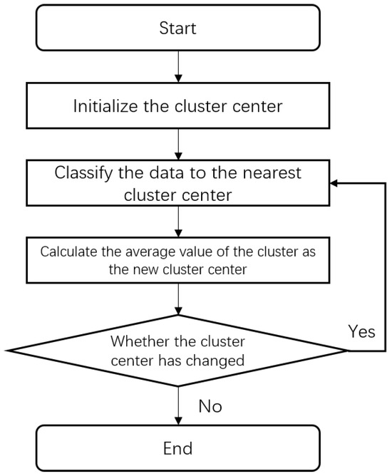
Figure 2. Flow chart of the K-Means clustering algorithm.

The FCM clustering algorithm first initializes the membership matrix and cluster centers. Then, it iteratively updates cluster centers and the membership matrix, minimizing the objective function until convergence, when either the maximum iterations are reached or the change in membership values falls below a set threshold [64,65]. As shown in Figure 3, the FCM algorithm workflow is illustrated.

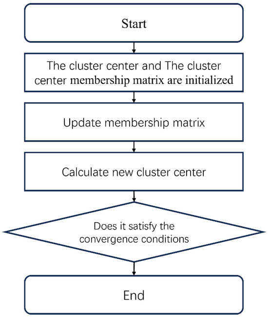
Figure 3. Flow chart of the FCM clustering algorithm.

The GMM is a probabilistic generative model that describes the overall data distribution by estimating the means, covariance matrices, and mixture weights of component Gaussian distributions. It classifies samples by maximizing the log-likelihood function [66]. As shown in Figure 4, the GMM algorithm workflow is presented.

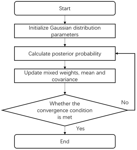
Figure 4. Flow chart of the GMM clustering algorithm.

The first step is to initialize the number of clusters k. Then, the posterior probability of each sample belonging to each cluster is calculated. The model parameters, including means, covariance matrices, and mixture weights, are updated accordingly. Using these parameters, the class probabilities are recalculated. This process iteratively refines the Gaussian parameters and computes the log-likelihood until its rate of change falls below a set threshold.

3.2.4. Classification Result Comparison Method

Unsupervised learning methods do not rely on pre-labeled data but do require the number of clusters to be specified in advance. The elbow method offers a systematic way for determining the optimal cluster number.

The elbow method calculates the within-cluster sum of squares for candidate cluster numbers, which is defined as the aggregate of squared Euclidean distances from each sample point to its respective cluster center. Finally, the number of clusters corresponding to the inflection point in the curve is selected as the optimal cluster number. The calculation formula for the within-cluster sum of squares is presented as follows [23]:

$$SSE={\displaystyle \sum _{i=1}^k{\displaystyle \sum _{p\in C_i}{\left|p-m_i\right|}^2}}.$$

(15)

where SSE denotes the within-cluster sum of squares, C_i represents the i-th cluster, k denotes the total number of clusters, m_i represents the centroid of cluster C_i, and p refers to the sample points in C_i excluding the centroid.

The silhouette coefficient is a widely used metric for assessing clustering quality, which simultaneously considers both intra-cluster cohesion and inter-cluster separation. The range of values for the silhouette coefficient typically falls between −1 and 1, signifying that better clustering performance is associated with higher values. By comparing the results of the three clustering algorithms using the silhouette coefficient, the appropriateness of the classification of core pore structure parameters can be assessed. The silhouette coefficient for each data point is calculated based on a formula, and the average of all data point silhouette coefficients is given as the silhouette coefficient for the clustering results. The formula is given below [67].

$$s(i)={\displaystyle \frac{b(i)-a(i)}{\max \left(a(i),b(i)\right)}}.$$

(16)

where a(i) signifies the mean distance between data point “i” and all other points in the same cluster, and b(i) refers to the mean distance from data point “i” to all points in the nearest neighboring cluster.

3.3. Prediction via Well Logs of Reservoir Pore Structure by DNNs

The aforementioned pore structure parameters of core samples can be used to accurately classify reservoirs. However, due to the difficulty of obtaining core samples and the high cost of laboratory testing, many wells lack sufficient pore structure data for effective reservoir classification and evaluation. Logging data serve as an indirect means of assessing reservoir pore structure parameters, providing continuous logging curves that reflect pore structure characteristics. This approach offers abundant data at comparatively low cost. Therefore, in this study, the reservoir classification results derived from pore structure parameters were used as labels and combined with corresponding logging data at the same depths to train a DNN model for predicting reservoir classifications based on logging curves.

A DNN is a type of feedforward neural network featuring multiple hidden layers that autonomously learns complex patterns from large datasets. Mimicking the human brain’s neural structure, it extracts relevant features directly from raw input data for advanced processing and decision-making [68]. A typical DNN architecture includes an input layer, multiple hidden layers, and an output layer. The input layer acquires external data and delivers it to the first hidden layer. Each hidden layer processes signals using neurons and activation functions, forwarding results to the following layer. This process persists until the final hidden layer transmits its output to the output layer, generating the network’s final output.

The workflow of a DNN is illustrated in Figure 5. The iterative optimization process of the network primarily consists of the following three key stages: forward propagation, in which activation functions are applied layer by layer to generate prediction values at the output layer; construction of a loss function to quantify model errors based on the difference between the predicted values and actual labels; and updating of network weight gradients through the backpropagation algorithm. These three steps are repeated iteratively, progressively adjusting the network parameters until either the convergence criteria, such as a preset accuracy threshold, are satisfied or the maximum iteration count is attained.

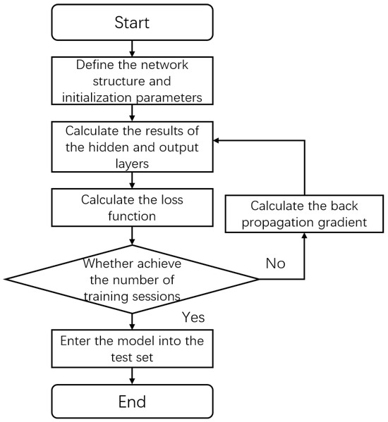
Figure 5. Flow chart of the DNN.

The computational process of neural networks takes place at the nodes, as expressed in [69]

$$Z=({\omega }^{T}x+\mathrm{b}).$$

(17)

where Z represents the output propagated forward, ω denotes the neuron’s weight vector, x is the input feature vector, and b signifies the bias term. Z is calculated as the sum of the weighted input features and the bias and is then propagated to the next layer. The weight vector ω defines the influence of each input on the neuron’s output, while the input vector x represents the features or activation values fed into the neuron. After model training and prediction, the loss function is calculated to evaluate result quality. For classification tasks, the cross-entropy loss is commonly used and is defined as follows [70]:

$$loss=-{\displaystyle \sum _{\mathrm{i}=1}^{\mathrm{C}}{\mathrm{y}}_i\log \left(z_i\right)}.$$

(18)

where y represents the true values, c denotes the number of classes, and z refers to the predicted outputs.

The cross-entropy loss function is effective for classification tasks, especially with imbalanced datasets, as it places greater emphasis on hard-to-classify samples, improving the model’s performance on them.

After obtaining the loss function, backpropagation is performed to update the network parameters. The most commonly used optimization approach is the gradient descent algorithm. Gradient descent updates the network weights and bias parameters to minimize the loss function by calculating the gradient of the loss function with respect to each parameter. The adjustments to these parameters are determined by using hyperparameters like the learning rate. The ultimate goal is to reduce the loss function and train the model effectively. The equation for the gradient descent algorithm is as follows [71]:

$$W_{ij}^L={\displaystyle \frac{\partial J}{\partial W_{ij}^L}}={\delta }_j^L{a}_i^{L-1}.$$

(19)

$$b_j^L={\displaystyle \frac{\partial J}{b_j^L}}={\delta }_j^L$$

(20)

where δ_j^L is defined as the error term between the predicted value and the true value, J denotes the loss function, W_ij^L represents the connection weight between output layer neuron j and the preceding layer neuron i, a_i^L−1 denotes the output value of the preceding layer neuron i, and b_j^L is the bias of the output layer neuron j.

3.4. DNN Reservoir Classification Prediction Model

This study utilizes six conventional well-logging curves, GR, DEN, CNL, DT, M2RX or RD, and M2R3 or RM, along with core-derived classification results as input data for the deep learning network, with the logging curve values having undergone standardized preprocessing.

Given the limited dataset in this study, employing a single hidden layer suffices to achieve the experimental objectives while reducing computational complexity. In preliminary experiments, we progressively decreased the learning rate within the range of 0.1 to 0.01, while comparing batch sizes of 16, 32, and 64. The results indicate that the optimal combination of model fitting accuracy and training efficiency is achieved when the learning rate is set to 0.01 and the batch size is 32.

The DNN designed in this study consists of three hidden layers. The number of neurons significantly affects both the computational complexity and the convergence speed of the model. To promote efficient convergence, the neuron quantity in each successive hidden layer is reduced. Specifically, the first hidden layer contains 64 neurons, and the neuron count is halved in each of the subsequent two layers. The first two hidden layers employ the ReLU activation function to maintain computational efficiency, while the Softmax activation function is applied in the final hidden layer to improve classification performance. The ReLU function accelerates network training, whereas the Softmax function reduces overfitting and enhances the network’s generalization capability.

The weight matrix was initialized using the Gaussian random initialization method, while the bias matrix was initialized to zero. After initialization, the activation function for the hidden layers was set, and gradient descent was selected as the optimization method for backpropagation. The cross-entropy loss function was employed as the loss function, with the learning rate set to 0.01. After each iteration, the training and test sets were shuffled and regrouped to prevent overfitting and ensure that the model could learn from all label parameters. The training process continued until the change in the loss function fell below a specified threshold or the predefined number of iterations was reached. Finally, the trained network was applied to the training and test sets from the final iteration.

4. Results

4.1. Porosity, Permeability, and Pore Structure Parameters of the Samples

Figure 6 shows the histogram of rock porosity and permeability distribution. It can be seen from the figure that porosity is distributed between 0.3% and 10.7% (Figure 6a), with the highest frequency of porosity distribution in the range of 4% to 6%, with an average porosity of 5.94%. The permeability is distributed between 0.01 mD and 10 mD (Figure 6b), with the highest frequency of distribution in the range of 0.01 mD to 1.0 mD, with an average permeability of 0.818 mD, which indicates that the Jurassic Ahe Formation reservoir in the Dibei area is a typical tight reservoir.

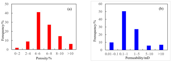
Figure 6. Histogram of porosity and permeability of core samples. (a) Histogram of porosity; (b) histogram of permeability.

Displacement pressure, the sorting coefficient, and skewness were chosen for histogram analysis. The three parameters shown in Figure 7 are used to characterize the sorting, size, and connectivity of the pore structure. Displacement pressure is distributed between 0.3 and 0.6 MPa, the sorting coefficient ranges from 0.25 to 0.5, and skewness is primarily within the range of 0.25 to 0.5. As shown in Table 1, all the pore structure parameters of representative samples are presented.

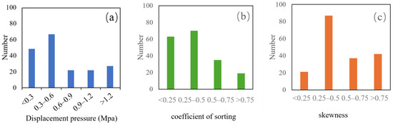
Figure 7. Histogram of pore structure parameters. (a) Displacement pressure; (b) coefficient of sorting; (c) skewness.

Table 1. Pore structure parameters of selected core samples in well YN2C.

Depth (m)	Lithology	Porosity (%)	Permeability (mD)	Median Stress (MPa)	Relative Sorting Coefficient	Max Throat Radius (um)	Sorting Coefficient	Displacement Pressure (MPa)	Structural Coefficient	Feature Structure Coefficient	Median Throat Radius (um)	Skewness	Uniformity Coefficient
4729.95	Coarse sandstone	5.6	0.324	4.947	1.101	1.501	0.298	0.500	3.599	0.252	0.151	1.809	0.271
4730.35	Breccia	9.0	29.4	1.404	1.193	5.863	0.823	0.128	0.349	2.397	0.534	1.891	0.689
4731.02	Breccia	3.9	0.385	3.936	1.022	1.550	0.330	0.484	3.057	0.319	0.190	1.642	0.323
4731.3	Fine-grained sandstone	3.5	1.154	12.68	1.393	0.729	0.259	1.029	3.196	0.224	0.059	2.363	0.185
4731.5	Gravelly coarse sandstone	4.9	0.3	6.151	1.337	0.818	0.257	0.916	2.096	0.356	0.121	2.353	0.192
4731.85	Gravelly coarse sandstone	7.1	0.955	2.772	1.026	1.720	0.370	0.436	2.581	0.377	0.270	1.644	0.360
4732.12	Gravelly coarse sandstone	7.4	1.18	2.080	1.046	2.349	0.466	0.319	2.981	0.320	0.360	1.589	0.446
4732.38	Gravelly coarse sandstone	7.2	1.35	2.145	1.026	2.210	0.450	0.339	2.627	0.370	0.349	1.630	0.438
4732.77	Medium sandstone	4.0	0.156	9.738	1.346	0.703	0.281	1.066	3.626	0.204	0.077	2.095	0.208
4733.26	Medium sandstone	3.7	0.111	14.84	1.113	0.677	0.151	1.107	2.348	0.382	0.050	1.851	0.135
4733.39	Medium sandstone	2.9	0.059	19.04	1.029	0.383	0.071	1.954	1.013	0.958	0.039	1.822	0.069
4733.6	Coarse sandstone	4.5	0.14	7.330	1.065	0.772	0.172	0.971	2.923	0.321	0.102	1.726	0.161
4733.86	Coarse sandstone	6.0	0.829	2.243	0.944	1.569	0.363	0.478	2.463	0.429	0.334	1.307	0.384
4734.25	Coarse sandstone	5.2	0.575	4.049	1.064	1.632	0.3198	0.459	2.281	0.4116	0.1852	1.774	0.1839
4729.95	Coarse sandstone	3.6	0.135	8.661	1.336	0.787	0.2475	0.953	3.047	0.2456	0.0865	2.353	0.2354

4.2. Results of Data Feature Extraction

In this study, the FZI is used as the reference sequence, and MICP parameters are the comparative sequences for evaluating their interrelationships. The rock samples from the study area were analyzed for pore structure parameters through grey relational analysis. Bigger correlation coefficients indicate stronger relationships between pore structure parameters and the FZI. Table 2 presents the grey relational analysis results, revealing that the following seven parameters exhibit particularly high correlation with FZI: relative sorting coefficient, displacement pressure, median pore-throat radius, sorting coefficient, structural coefficient, feature structural coefficient, and skewness. Consequently, these seven pore structure parameters were selected for subsequent application and analysis.

Table 2. Results of the grey association correlation analysis.

Relative Sorting Coefficient	Displacement Pressure (MPa)	Structural Coefficient	Sorting Coefficient	Median Pore-Throat Radius (um)
0.929	0.901	0.873	0.867	0.865
Feature Structure Coefficient	Skewness	Max Throat Radius (um)	Uniformity Coefficient	Median Stress (MPa)
0.864	0.836	0.804	0.757	0.656

Figure 8 presents the changes in eigenvalues with the number of principal components obtained from the PCA of pore structure parameters. Table 3 presents the eigenvalues and contribution rates. Larger eigenvalues indicate that the associated principal components capture a higher proportion of variance and information in the original dataset. In practical applications, principal components featuring substantially large eigenvalues and cumulative contribution rates exceeding a specified threshold are typically selected as the basis for analysis. As shown in Figure 8 and Table 3, the variance contribution rate of the fourth principal component exhibits a significant decline, and the cumulative variance contribution rate has plateaued after the first three principal components. This characteristic clearly indicates that the first three principal components fully capture the most essential and discriminative feature information within the original data. Including the fourth principal component offers negligible improvement in the clustering results. On the contrary, introducing redundant dimensions would increase computational complexity and reduce classification efficiency. In this study, the threshold was set at 80%, and the three principal components with the highest eigenvalues were selected, achieving a cumulative contribution rate of 85%. This threshold is a commonly used empirical value in multivariate statistical analysis, achieving a good balance between retaining core information and reducing data dimensions. These three components effectively represent the characteristics of the original data while reducing data redundancy and multicollinearity.

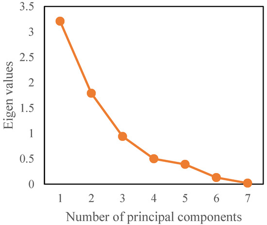
Figure 8. Changes in eigenvalues with the number of principal components.

Table 3. Eigenvalues for the PCA.

Number	Eigenvalues	Proportion of Information Contained (%)
1	3.21	45.85
2	1.79	71.52
3	0.94	85.00
4	0.50	92.20
5	0.39	97.82
6	0.13	99.70
7	0.02	100

4.3. Classification of Pore Structure

Using the K-Means method, the samples are divided into two to eight groups, and with the within-cluster sum of squares value calculated for each classification, the three principal components obtained from the PCA were applied to Equation (15) to generate an elbow method plot (Figure 9). Based on the observed inflection point, where the rate of SSE reduction markedly decreased beyond this value, the optimal number of clusters was determined to be three.

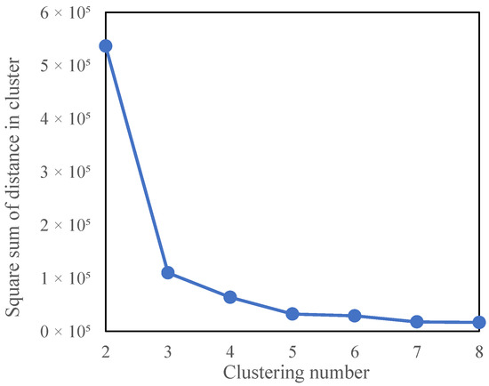
Figure 9. Plot of elbow method.

The three principal components extracted earlier were classified using K-Means, FCM, and GMM clustering methods, resulting in three distinct clustering outcomes. As shown in Table 4, all three algorithms produced positive silhouette coefficients, confirming the validity of the classifications.

Table 4. The contour coefficients of the clustering algorithms.

Clustering Algorithm	Silhouette Coefficient
K-Means	0.448
FCM	0.305
GMM	0.532

The K-Means algorithm demonstrates computational efficiency and low complexity. Through appropriate initialization methods and parameter optimization, it achieves relatively high silhouette coefficients, resulting in satisfactory clustering performance. The FCM algorithm employs fuzzy logic principles to determine clusters based on membership degrees, producing stable classification outcomes that show minimal sensitivity to initial centroid selection. However, FCM is sensitive to outliers, and when anomalous data points are present in the sample set, the calculated silhouette coefficient tends to be lower. The GMM operates on the fundamental assumption that the data originate from a mixture of multiple Gaussian distributions. By employing the Expectation–Maximization algorithm for parameter estimation, the GMM effectively handles complex data distributions and noise interference while avoiding convergence to local maxima caused by isolated points. Consequently, the GMM consistently produces the highest silhouette coefficients among the three methods. The silhouette coefficients for all three clustering results are positive values, indicating that the classification results are valid. This study uses pore connectivity as the classification criterion; lower silhouette coefficient values suggest that the classification of stratigraphic pore structure characteristics lacks clear boundaries, with rocks of different pore structures exhibiting similar seepage capabilities. According to the voting scheme, the majority category among the three clustering results was adopted as the overall classification outcome. When classification results from different methods conflict, the classification result derived from the method with the highest contour coefficient is adopted. Representative classification results are presented in Table 5.

Table 5. Classification of selected samples.

Sample Depth (m)	K-Means Clustering Algorithm	FCM Clustering Algorithm	GMM Clustering Algorithm	Final Classification
4729.95	1	1	1	1
4730.35	2	2	2	2
4731.02	3	2	3	3
4731.3	3	3	3	3
4731.5	2	2	2	2
4731.85	2	3	2	2
4732.12	2	3	2	2
4732.38	3	2	2	2
4732.77	3	2	3	3
4733.26	1	1	2	1
4733.39	1	1	2	1
4733.6	2	2	2	2
4733.86	1	1	2	1
4734.25	2	3	3	3
4729.95	3	3	3	3

Given the substantial number of mercury injection curves, this study presents representative capillary pressure curves for three types of classification and images of cast plates for the three types of classification (Figure 10). The cumulative capillary pressure curves for each category are also plotted. Additionally, the cumulative mercury saturation curves corresponding to the three pore structure categories are shown in Figure 11. Among these, Type I exhibits the most favorable pore structure, with an average maximum mercury saturation of 83.7% and a peak value of 96.3%. Type II follows, with an average maximum mercury saturation of 73.8% and a maximum value of 85.6%. Type III displays the least favorable pore structure, with an average maximum mercury saturation of 59.5% and a maximum value of 73.3%. Based on significant differences in cumulative mercury saturation, the distinct characteristics of the three pore structures in terms of porosity, permeability, and flow behavior can be further clarified. Regarding porosity, Type I exhibits high mercury saturation, indicating well-developed pore spaces with excellent connectivity, resulting in the highest porosity among the three types; Type II exhibits moderate development with correspondingly lower porosity; and Type III features scarce interconnected pathways and a high proportion of isolated pores, resulting in the lowest porosity. Permeability is closely correlated with pore-throat radius and connectivity. Type I exhibits coarse throats and well-sorted pore structures, enabling unobstructed flow pathways and delivering the highest permeability. Type II features reduced throat radii and diminished connectivity, resulting in decreased permeability. Type III possesses narrow throats and poor connectivity, hindering the formation of effective flow pathways and yielding the lowest permeability. Regarding flow behavior, Type I exhibits the lowest displacement pressure and highest permeability, with minimal seepage resistance during fluid flow, enabling rapid and uniform passage through the pore network. Type II features moderate displacement pressure and permeability, where fluid flow is readily constrained by localized narrow throats, resulting in lower seepage rates than Type I. Type III exhibits very high displacement pressure and extremely low permeability, presenting significant flow resistance. Fluid flow only commences upon reaching the critical pressure threshold. This flow pattern is intrinsically consistent with the conclusion drawn by Zou et al. (2025) that the initial fracture angle influences gas flow processes [72]. It not only confirms the critical role of pore structure type in controlling reservoir permeability but also further supports the geological plausibility of the clustering results. The capillary pressure curves reveal clear distinctions among the three reservoir types, demonstrating that reservoir classification using clustering methods is effective.

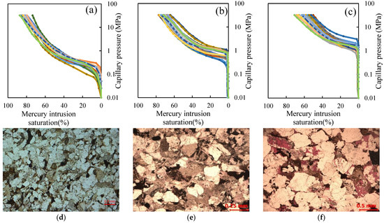
Figure 10. Capillary pressure curves of three types of reservoirs. Curves of different colors represent the capillary pressure curves of different rock samples. (a) The first type of MICP curve; (b) the second type of MICP curve; (c) the third type of MICP curve; (d) the first type of casting thin section; (e) the second type of casting thin section; (f) the third type of casting thin section.

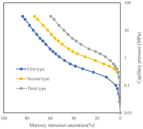
Figure 11. Cumulative capillary pressure curves for three different types of reservoirs.

4.4. DNN Reservoir Classification Prediction

After inputting the training and test sets into the model, the training set achieved an accuracy rate of 88.2%, while the test set achieved 80.43%. Overall, the prediction results demonstrated relatively high accuracy. The corresponding confusion matrices are presented in Figure 12 and Figure 13. From the figures, confusion matrices are used to illustrate classification accuracy. The vertical axis displays the classification results obtained from rock experimental data after clustering computation, while the horizontal axis shows the classification outcomes predicted by the neural network. Categories marked with diagonal lines indicate correct predictions. In the diagram, correct predictions are highlighted in blue and incorrect ones in red. The precision rate is marked in blue at the bottom of the image, and the recall rate is marked in blue on the right side of the image. The F1 scores of the training set are 0.865, 0.866, and 0.917, and those of the test set are 0.812, 0.817, and 0.762. The 95% CI for the training set is 79% to 92%, and the 95% CI for the test set is 79% to 94%. It can be seen that the accuracy distribution of each category on the training set is relatively even, indicating that the neural network’s learning ability for different categories is relatively balanced. On the test set, the classification performance of category 2 is better than other categories, indicating that the features of category 2 are more prominent in the test set samples, or the model is more easily recognizable for this category.

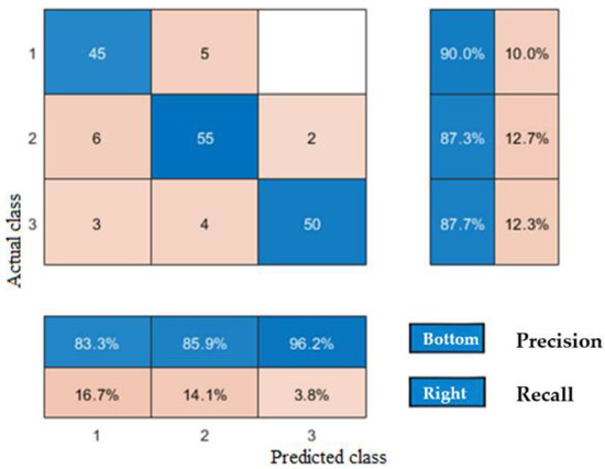
Figure 12. Confusion matrices for the training sets.

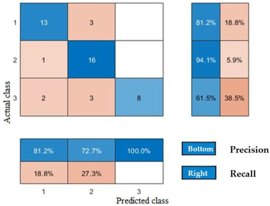
Figure 13. Confusion matrices for the test sets.

Based on a further analysis of the confusion matrix, Type III reservoirs exhibit high precision but low recall. This indicates that while these samples achieve high recognition rates during the learning phase, their relatively small sample size may cause the model to prioritize fitting majority-class features during classification. Consequently, they are more likely to be misclassified as other types. This reflects the complex pore structure and extreme heterogeneity of Type III reservoirs, which often contain localized anomalies such as microfractures and high-resistance mineral bands. In conventional logging curves, these minute anomalies within tight layers can generate logging responses similar to those of high-quality reservoirs, leading to confusion in model classification. In contrast, both precision and recall rates are higher for Type I and Type II reservoirs.

To validate the effectiveness of the trained model in practical applications, this study applied the deep learning model to the logging curve analysis of the high-productivity well YN2C and the low-productivity well YN4. The prediction results are presented in Figure 14 and Figure 15. In these figures, the first track is depth, the second track, GR, is the natural gamma log, the third track, DT, is the acoustic log, CNL is the Neutron Porosity log, and DEN is the density log. The fourth track has three resistivity curves for deep, medium, and shallow; the fifth track compares the predicted classifications with the core-derived classifications. The second track reflects the lithology of the reservoir, the third one reflects the physical properties of the stratum, and the fourth one reflects the oil-bearing characteristics of the reservoir. In the fifth track, the purple regions represent Type I reservoirs with good pore structure, the green regions represent Type II reservoirs with moderate pore structure, and the red regions represent Type III reservoirs with relatively poor pore structure. The results show that the predicted classifications align well with the core classifications.

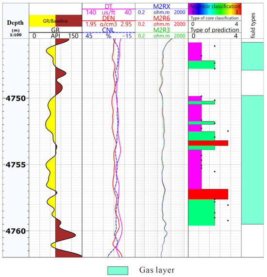
Figure 14. Classification results of well YN2C. The GR, DT, DEN, CNL, M2RX, and M2R3 are input logs. The purple, green, and red regions in track five represent Type I, II, and III predictions. The dots in this track are classifications of core samples.

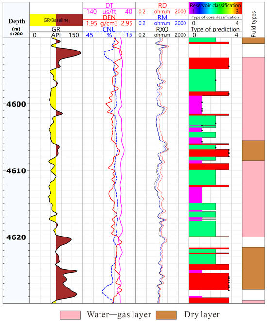
Figure 15. Classification results of well YN4. The GR, DT, DEN, CNL, RD, and RM are input logs.

Furthermore, the proportions of each classification within the different gas-bearing reservoirs (gas layer, water–gas interlayer, and dry layer) of the three wells were statistically analyzed, as shown in Table 6. Gas layers are primarily distributed in Type I and Type II reservoirs, which have relatively good pore structures that facilitate the storage and flow of hydrocarbons. In contrast, poor gas layers are mainly composed of Type II reservoirs, though they also include some Type III reservoirs. Dry layers are primarily composed of Type II and Type III reservoirs, reflecting relatively poor pore structures in these intervals. When comparing individual wells, the high-productivity well YN2C predominantly constitutes Type I and Type II reservoirs, indicating an overall favorable pore structure in the reservoir. In the low-productivity well YN4, the water-bearing gas layer also primarily consists of Type I and Type II reservoirs, while the dry layer contains a relatively higher proportion of Type III reservoirs.

Table 6. Proportion of each pore structure type in different layers.

Layers	Proportion of Type I (%)	Proportion of Type II (%)	Proportion of Type III (%)
Gas layer	53.5	34.6	11.8
Water–gas layer	30.6	51.3	17.9
Dry layer	7.1	31.7	61.1

5. Discussion

This paper presents a methodology for predicting the pore structure of deep tight sandstones based on conventional logging data and machine learning approaches. The pore structure parameters are derived from capillary pressure data of core samples. And the classification was further conducted using K-Means, FCM, and GMM clustering methods. By inputting the results of pore structure classification into a deep neural network (DNN) model, we predict reservoir pore structure categories with conventional well logs. The purpose of this article is to propose an integrated workflow for pore structure prediction, not to prove which ML methods to choose. Thus, the three clustering methods could be replaceable. The DNN method could be replaced by any ML approach if the accuracy is higher. The error of the MICP measurements may have influence on the pore structure prediction, but this could not be avoided and is hard to quantify. The use of machine learning algorithms for prediction has the limitation of quantity and representativeness of samples, which exposes models to the risk of overfitting and insufficient generalization capabilities in heterogeneous reservoirs. Therefore, prior to training, the study strictly maintained distributional proximity among different sample types to prevent models from overfitting to training set noise. When directly transferring this model to deep tight sandstone reservoirs across different blocks and stratigraphic levels, prediction accuracy may decline to varying degrees. Subsequent optimization of the prediction model can be achieved by expanding the core sample set across blocks and stratigraphic levels.

This study used machine learning to analyze the relationship between pore structure parameters and logging values. Compared with the traditional pore structure prediction method, this method reduces the complex derivation process and reduces the calculation complexity by feature mapping. The experimental verification phase focuses on empirical research in the DB region. In the future, this research area will be gradually expanded in accordance with the principle of multi-region and multi-model verification, and machine learning algorithms with different principles will be introduced for comparative verification.

6. Conclusions

The primary conclusions are summarized as follows:

(i) Using the capillary pressure curves obtained through laboratory measurements, the pore structure parameters of the reservoir rock samples were processed. Through sensitivity analysis and dimensionality reduction, these parameters were transformed into three principal component variables. Subsequently, K-Means, FCM, and GMM clustering methods were applied to classify the core samples. The capillary pressure curves of the resulting categories exhibited significant differences across all parameters.

(ii) Using the core classification results as labels and six conventional logging curves as input data, a pore structure classification prediction model was trained with a DNN. The model achieved an accuracy of 88.2% on the validation set and 80.4% on the test set, demonstrating that the proposed method provides high predictive accuracy.

(iii) The results of applying the neural network model to reservoir prediction indicate that gas zones are predominantly classified as Type I reservoirs with optimal pore structures. Poor gas zones are mainly composed of Type II reservoirs with moderate pore structures, while dry zones are primarily classified as Type III reservoirs with poor pore structures. The predicted reservoir category is consistent with the interpretation conclusion.

(iv) The DNN model has demonstrated promising results in tight sandstone reservoirs within this region. The use of machine learning algorithms for prediction has the limitation of quantity and representativeness of samples. Future research could employ the convolutional neural network (CNN) and other interpretable methods or explore their application in other tight sandstone structures with larger datasets to refine neural network models for application across diverse geological formations.

References

- Tian, J. Petroleum exploration achievements and future targets of Tarim basin. Xinjiang Pet. Geol. 2019, 40, 1–11. [Google Scholar] [CrossRef]
- Mangi, H.N.; Chi, R.; DeTian, Y.; Sindhu, L.; He, D.; Ashraf, U.; Fu, H.; Zixuan, L.; Zhou, W.; Anees, A. The ungrind and grinded effects on the pore geometry and adsorption mechanism of the coal particles. J. Nat. Gas Sci. Eng. 2022, 100, 104463. [Google Scholar] [CrossRef]
- Mirzaei-Paiaman, A.; Sabbagh, F.; Ostadhassan, M.; Shafiei, A.; Rezaee, R.; Saboorian-Jooybari, H.; Chen, Z. A further verification of FZI* and PSRTI: Newly developed petrophysical rock typing indices. J. Pet. Sci. Eng. 2019, 175, 693–705. [Google Scholar] [CrossRef]
- Wang, L.; Liu, B.; Bai, L.; Yu, Z.; Huo, Q.; Gao, Y. Pore evolution modeling in natural lacustrine shale influenced by mineral composition: Implications for shale oil exploration and CO2 storage. Adv. Geo-Energy Res. 2024, 13, 218–230. [Google Scholar] [CrossRef]
- Wang, L.; Zhao, N.; Sima, L.; Meng, F.; Guo, Y. Pore structure characterization of the tight reservoir: Systematic integration of mercury injection and nuclear magnetic resonance. Energy Fuels 2018, 32, 7471–7484. [Google Scholar] [CrossRef]
- Wang, X.; Hou, J.; Liu, Y.; Zhao, P.; Ma, K.E.; Wang, D.; Ren, X.; Yan, L.I.N. Overall psd and fractal characteristics of tight oil reservoirs: A case study of lucaogou formation in junggar basin, China. Fractals 2019, 27, 1940005. [Google Scholar] [CrossRef]
- Duan, C.; Deng, J.; Li, Y.; Lu, Y.; Tang, Z.; Wang, X. Effect of pore structure on the dispersion and attenuation of fluid-saturated tight sandstone. J. Geophys. Eng. 2018, 15, 449–460. [Google Scholar] [CrossRef]
- Su, Y.; Zha, M.; Ding, X.; Qu, J.; Wang, X.; Yang, C.; Iglauer, S. Pore type and pore size distribution of tight reservoirs in the Permian Lucaogou Formation of the Jimsar Sag, Junggar Basin, NW China. Mar. Pet. Geol. 2018, 89, 761–774. [Google Scholar] [CrossRef]
- Zhao, P.; Wang, Z.; Sun, Z.; Cai, J.; Wang, L. Investigation on the pore structure and multifractal characteristics of tight oil reservoirs using NMR measurements: Permian Lucaogou Formation in Jimusaer Sag, Junggar Basin. Mar. Pet. Geol. 2017, 86, 1067–1081. [Google Scholar] [CrossRef]
- Xin, Y.; Wang, G.; Liu, B.; Ai, Y.; Cai, D.; Yang, S.; Liu, H.; Xie, Y.; Chen, K. Pore structure evaluation in ultra-deep tight sandstones using NMR measurements and fractal analysis. J. Pet. Sci. Eng. 2022, 211, 110180. [Google Scholar] [CrossRef]
- Cnudde, V.; Boone, M.N. High-resolution X-ray computed tomography in geosciences: A review of the current technology and applications. Earth Sci. Rev. 2013, 123, 1–17. [Google Scholar] [CrossRef]
- Malakhov, A.O.; Saifullin, E.R.; Al-Janabi, O.; Bykov, A.O.; Zharkova, D.I.; Nazarychev, S.A.; Zharkov, D.A.; Kadyrov, R.I.; Nguyen, T.H.; Varfolomeev, M.A. Dynamic adsorption of sulfate propoxylate and alkylbenzene sulfonate surfactants: Correlation with 3d pore geometry in highly heterogeneous high-salinity carbonate reservoirs. Arab. J. Sci. Eng. 2025, 50, 10489–10506. [Google Scholar] [CrossRef]
- Yang, C.; Yang, E. Mineral composition and pore structure on spontaneous imbibition in tight sandstone reservoirs. Sci. Rep. 2025, 15, 7504. [Google Scholar] [CrossRef]
- Labani, M.M.; Rezaee, R.; Saeedi, A.; Hinai, A.A. Evaluation of pore size spectrum of gas shale reservoirs using low pressure nitrogen adsorption, gas expansion and mercury porosimetry: A case study from the Perth and Canning Basins, Western Australia. J. Pet. Sci. Eng. 2013, 112, 7–16. [Google Scholar] [CrossRef]
- Yang, Q.L.; Li, A.Q.; Sun, Y.N.; Cui, P.F. Classification method for extra-low permeability reservoirs. Lithol. Reserv. 2007, 4, 51–56. [Google Scholar] [CrossRef]
- Ge, H. Classifcation method and evaluation of flow unit in low porosity and permeability reservoir. Offshore Oil 2016, 36, 45–50. [Google Scholar] [CrossRef]
- Xiao, L.; Mao, Z.Q.; Zou, C.C.; Jin, Y.; Zhu, J.C. A new methodology of constructing pseudo capillary pressure (Pc) curves from nuclear magnetic resonance (NMR) logs. J. Pet. Sci. Eng. 2016, 147, 154–167. [Google Scholar] [CrossRef]
- Xu, Z.; Zhao, P.; Wang, Z.; Ostadhassan, M.; Pan, Z. Characterization and consecutive prediction of pore structures in tight oil reservoirs. Energies 2018, 11, 2705. [Google Scholar] [CrossRef]
- Wu, H.P.; Wang, Z.W.; Xu, F.H.; Cui, Y.T.; Yu, H. Pore structure evaluation of volcanic reservoir of the 2nd Member of Huoshiling Formation in Wangfu fault depression. Glob. Geol. 2021, 40, 100–106+124. [Google Scholar] [CrossRef]
- Wang, Y.X.; Xie, B.; Lai, Q.; Zhao, Z.A.; Xia, X.Y.; Xie, R.H. Evaluation of pore structure and classification in tight gas reservoir based on NMR logging. Prog. Geophys. 2023, 38, 759–767. [Google Scholar] [CrossRef]
- Zhou, J.; Liu, B.; Shao, M.; Song, Y.; Ostadhassan, M.; Yin, C.; Liu, J.; Jiang, Y. Pore structure analysis and classification of pyroclastic reservoirs in the Dehui fault depression based on experimental and well-logging data. Geoenergy Sci. Eng. 2023, 224, 211620. [Google Scholar] [CrossRef]
- Peng, J.; Han, H.; Xia, Q.; Li, B. Evaluation of the pore structure of tight sandstone reservoirs based on multifractal analysis: A case study from the Kepingtage Formation in the Shuntuoguole uplift, Tarim Basin, NW China. J. Geophys. Eng. 2018, 15, 1122–1136. [Google Scholar] [CrossRef]
- Iraji, S.; Soltanmohammadi, R.; Matheus, G.F.; Basso, M.; Vidal, A.C. Application of unsupervised learning and deep learning for rock type prediction and petrophysical characterization using multi-scale data. Geoenergy Sci. Eng. 2023, 230, 212241. [Google Scholar] [CrossRef]
- Wu, H.; Liu, R.E.; Ji, Y.L.; Zhang, C.L.; Zhou, Y.; Zhang, Y.Z. Classification of pore structures in typical tight sandstone gas reservoir and its significance: A case study of the He8 Member of Upper Palaeozoic Shihezi Formation in Ordos Basin, China. Nat. Gas. Geosci. 2016, 27, 835–843. [Google Scholar] [CrossRef]
- An, X.; Wang, D.S.; Xiang, L.P.; Wang, Z.Q.; Zhang, G.S. Cluster analysis of pore structure characteristics of tight oil reservoir—A case study in Lucaogou formation of Jimusar Sag. Reserv. Eval. Dev. 2016, 6, 7–13. [Google Scholar] [CrossRef]
- Zhao, X.Y.; Wang, Z.Q. The characteristic of K2d reservoir pore structure and its evaluation in the middle zone of southern Junggar basin. Sci. Technol. Eng. 2017, 17, 49–56. [Google Scholar] [CrossRef]
- Wang, J.; Zhang, C.M. Pore structures and classification of carbonate reservoirs in the middle east. Well Log. Technol. 2019, 43, 631–635. [Google Scholar] [CrossRef]
- Chen, P.; Wang, X.; Guo, L. Complex pore structure geological modeling of carbonate reservoirs: A case of M formation of B oilfield in Missan Oilfields, Iraq. Sci. Technol. Eng. 2019, 19, 81–89. [Google Scholar] [CrossRef]
- Lu, Y.; Liu, Z.B.; Liao, X.W.; Li, C.; Li, Y. Automatic classification of pore structures of low-permeability sandstones based on self-organizing-map neural network algorithm. Bull. Geol. Sci. Technol. 2024, 43, 318–330. [Google Scholar] [CrossRef]
- Lin, J.L.; Nie, J.; Li, P.J.; Yang, Y. Micropore structure type identification based on BP neural network. Well Log. Technol. 2009, 33, 355–359. [Google Scholar] [CrossRef]
- Sun, X.X. On Classification and evaluation of extra-low porosity and permeability reservoir in Yongjin oilfield, Dzungaria Basin. Well Log. Technol. 2012, 36, 479–484. [Google Scholar] [CrossRef]
- Liu, X.D.; Zheng, W.; Ma, X.L. Study on pore structure of Hanjiang Formation sandstone reservoir in A area of Yangjiang sag. Chin. Energy Environ. Prot. 2023, 45, 216–223. [Google Scholar] [CrossRef]
- Zhang, X.B.; Cheng, G.D.; Zhao, J.L.; Dai, W.X.; Tao, Y. Research on classification and evaluation of Chang 3 reservoir in H area based on BP neural network technology. Prog. Geophys. 2023, 38, 1272–1281. [Google Scholar] [CrossRef]
- Song, Z.; Qian, Y.; Mao, Y.; Chen, X.; Ranjith, P.G.; Deng, Q. Artificial intelligence-based investigation of fault slip induced by stress unloading during geo-energy extraction. Adv. Geo-Energy Res. 2024, 14, 106–118. [Google Scholar] [CrossRef]
- Liao, G.Z.; Li, Y.Z.; Xiao, L.Z.; Qin, Z.J.; Hu, X.Y.; Hu, F.L. Prediction of microscopic pore structure of tight reservoirs using convolutional neural network mode. Petrol. Sci. Bull. 2020, 5, 26–38. [Google Scholar] [CrossRef]
- Han, B.H. Study on Logging Evaluation Method of Glutenite Reservoir in Niudong Area, Northern Margin of Qaidam Basin. Master’s Thesis, Chang’an University, Xi’an, China, 2021. [Google Scholar] [CrossRef]
- Yang, T.; Tang, H.; Dai, J.; Wang, H.; Wen, X.; Wang, M.; He, J.; Wang, M. Quantitative classification and prediction of pore structure in low porosity and low permeability sandstone: A machine learning approach. Geoenergy Sci. Eng. 2025, 247, 213708. [Google Scholar] [CrossRef]
- Tang, X.M.; Yin, X.S.; LÜ, Y.J.; Song, Y.J.; Chen, X.Y.; Yi, J. Determination of permeability of medium-low porosity and extra-low permeability reservoirs based on pore structure reservoir classification: A case study of S reservoir in block B. Prog. Geophys. 2023, 38, 271–284. [Google Scholar] [CrossRef]
- Ding, Q.; Gan, L.; Wei, L.; Zhang, Y.; Yang, H.; Jiang, X.; Wang, Y. The dual pore structure factors and its application in seismic prediction of reservoir permeability. Acta Petrol. Sin. 2023, 44, 339–347. [Google Scholar] [CrossRef]
- Ilyushin, Y.; Nosova, V. Development of mathematical model for forecasting the production rate. Int. J. Eng. 2025, 38, 1749–1757. [Google Scholar] [CrossRef]
- Abedini, M.; Ziaii, M.; Negahdarzadeh, Y.; Ghiasi-Freez, J. Porosity classification from thin sections using image analysis and neural networks including shallow and deep learning in Jahrum formation. J. Min. Environ. 2018, 9, 513–525. [Google Scholar] [CrossRef]
- Al-Mudhafar, W.J. Integrating well log interpretations for lithofacies classification and permeability modeling through advanced machine learning algorithms. J. Pet. Explor. Prod. Technol. 2017, 7, 1023–1033. [Google Scholar] [CrossRef]
- Tang, Y.G.; Yang, X.Z.; Xie, H.W.; Xu, Z.P.; Wei, H.X.; Xie, Y.N. Tight gas reservoir characteristics and exploration potential of jurassic ahe formation in kuqa depression, tarim basin. China Pet. Explor. 2021, 26, 113–124. [Google Scholar] [CrossRef]
- Zou, C.; Jia, J.; Tao, S.; Tao, X. Analysis of reservoir forming conditions and prediction of continuous tight gas reservoirs for the deep jurassic in the eastern kuqa depression, tarim basin. Acta Geol. Sin. 2011, 85, 1173–1186. [Google Scholar] [CrossRef]
- Liu, L.W.; Sun, X.W.; Zhao, Y.J.; Jin, J.N. Hydrocarbon distribution and accumulation mechanism of Dibei tight sandstone gas reservoir in Kuqa depression, Tarim Basin. Xinjiang Pet. Geol. 2016, 37, 257–261. [Google Scholar] [CrossRef]
- Li, D.; Wang, G.-W.; Bie, K.; Lai, J.; Lei, D.-W.; Wang, S.; Qiu, H.-H.; Guo, H.-B.; Zhao, F.; Zhao, X.; et al. Formation mechanism and reservoir quality evaluation in tight sandstones under a compressional tectonic setting: The Jurassic Ahe Formation in Kuqa Depression, Tarim Basin, China. Pet. Sci. 2025, 22, 998–1020. [Google Scholar] [CrossRef]
- Xu, C.; Torres-Verdín, C. Pore system characterization and petrophysical rock classification using a bimodal gaussian density function. Math. Geosci. 2013, 45, 753–771. [Google Scholar] [CrossRef]
- Li, Y.Z. Research on Reservoir Pore Structure Evaluation and Reservoir Classification Prediction Method Based on Deep Learning. Master’s Thesis, China University of Petroleum, Beijing, China, 2020. [Google Scholar] [CrossRef]
- Washburn, E.W. Note on a method of determining the distribution of pore sizes in a porous material. Proc. Natl. Acad. Sci. USA 1921, 7, 115–116. [Google Scholar] [CrossRef]
- Folk, R.L.; Ward, W.C. Brazos River bar [Texas]; a study in the significance of grain size parameters. J. Sediment. Res. 1957, 27, 3–26. [Google Scholar] [CrossRef]
- Liu, G.; Xie, S.; Tian, W.; Wang, J.; Li, S.; Wang, Y.; Yang, D. Effect of pore-throat structure on gas-water seepage behaviour in a tight sandstone gas reservoir. Fuel 2022, 310, 121901. [Google Scholar] [CrossRef]
- Wang, X.; Yang, S.; Zhao, Y.; Wang, Y. Improved pore structure prediction based on MICP with a data mining and machine learning system approach in Mesozoic strata of Gaoqing field, Jiyang depression. J. Pet. Sci. Eng. 2018, 171, 362–393. [Google Scholar] [CrossRef]
- Liu, Y.; Liu, Y.; Zhang, Q.; Li, C.; Feng, Y.; Wang, Y.; Xue, Y.; Ma, H. Petrophysical static rock typing for carbonate reservoirs based on mercury injection capillary pressure curves using principal component analysis. J. Pet. Sci. Eng. 2019, 181, 106175. [Google Scholar] [CrossRef]
- Yang, S.L.; Wei, J.Z. Reservoir Physics; Petroleum Industry Press: Beijing, China, 2004; ISBN 7-5021-4678-4. [Google Scholar]
- Jing, T.T.; Han, Y.N.; Shi, Y.K.; Ma, Y.N.; Wei, L.J.; Wang, M.X.; Guo, Y.Q. Study on flow unit of Yan91 reservoir in Y66 area of Jing’an oilfield. J. Hebei Geo Univ. 2021, 44, 32–36. [Google Scholar] [CrossRef]
- Amaefule, J.O.; Altunbay, M.; Tiab, D.; Kersey, D.G.; Keelan, D.K. Enhanced reservoir description: Using core and log data to identify hydraulic (flow) units and predict permeability in uncored intervals/wells. In Proceedings of the SPE Annual Technical Conference and Exhibition, Houston, TX, USA, 3–6 October 1993. SPE–26436–MS. [Google Scholar] [CrossRef]
- Abbaszadeh, M.; Fujii, H.; Fujimoto, F. Permeability prediction by hydraulic flow units—Theory and applications. SPE Form. Eval. 1996, 11, 263–271. [Google Scholar] [CrossRef]
- Zhou, Y.; Zhang, Q.; Bai, G.; Zhao, H.; Shuai, G.; Cui, Y.; Shao, J. Groundwater dynamics clustering and prediction based on grey relational analysis and LSTM model: A case study in Beijing Plain, China. J. Hydrol. Reg. Stud. 2024, 56, 102011. [Google Scholar] [CrossRef]
- Arıcı, E.; Keleştemur, O. Optimization of mortars containing steel scale using Taguchi based grey relational analysis method. Constr. Build. Mater. 2019, 214, 232–241. [Google Scholar] [CrossRef]
- Draper, B.A.; Baek, K.; Bartlett, M.S.; Beveridge, J.R. Recognizing faces with PCA and ICA. Comput. Vis. Image Underst. 2003, 91, 115–137. [Google Scholar] [CrossRef]
- Wu, B.-H.; Xie, R.H.; Xiao, L.Z.; Guo, J.F.; Jin, G.W.; Fu, J.W. Integrated classification method of tight sandstone reservoir based on principal component analysis–Simulated annealing genetic algorithm–fuzzy cluster means. Pet. Sci. 2023, 20, 2747–2758. [Google Scholar] [CrossRef]
- Chang, X.; Han, R.; Zhang, J.; Vandeginste, V.; Zhang, X.; Liu, Y.; Han, S. Prediction of coal body structure of deep coal reservoirs using logging curves: Principal component analysis and evaluation of factors influencing coal body structure distribution. Nat. Resour. Res. 2024, 34, 1023–1044. [Google Scholar] [CrossRef]
- Zhang, Z.; Chen, X.; Wang, C.; Wang, R.; Song, W.; Nie, F. Structured multi-view k-means clustering. Pattern Recognit. 2025, 160, 111113. [Google Scholar] [CrossRef]
- Estiri, H.; Abounia Omran, B.; Murphy, S.N. Kluster: An efficient scalable procedure for approximating the number of clusters in unsupervised learning. Big Data Res. 2018, 13, 38–51. [Google Scholar] [CrossRef]
- Wang, Z.H.; Wang, S.Y.; Du, H. Improved fuzzy C-means clustering algorithm based on density-sensitive distance. Comput. Eng. 2021, 47, 88–96+103. [Google Scholar] [CrossRef]
- Wang, W.D.; Xu, J.H.; Zhang, Z.F.; Yang, X.B. Gaussian mixture models algorithm based on density peaks clustering. Comput. Sci. 2021, 48, 191–196. [Google Scholar] [CrossRef]
- Bagirov, A.M.; Aliguliyev, R.M.; Sultanova, N. Finding compact and well-separated clusters: Clustering using silhouette coefficients. Pattern Recognit. 2023, 135, 109144. [Google Scholar] [CrossRef]
- Jiang, Y.Y.; Xia, L.; Jiang, B.Y.; Han, W.; Wang, K. Research on fault detection and localization system for wireless private network devices based on DNN-SVM. J. Test. Meas. Technol. 2024, 38, 435–440. [Google Scholar] [CrossRef]
- Veerasamy, V.; Wahab, N.I.A.; Othman, M.L.; Padmanaban, S.; Sekar, K.; Ramachandran, R.; Hizam, H.; Vinayagam, A.; Islam, M.Z. LSTM recurrent neural network classifier for high impedance fault detection in solar pv integrated power system. IEEE Access. 2021, 9, 32672–32687. [Google Scholar] [CrossRef]
- Polat, G.; Çağlar, Ü.M.; Temizel, A. Class distance weighted cross entropy loss for classification of disease severity. Expert. Syst. Appl. 2025, 269, 126372. [Google Scholar] [CrossRef]
- Yang, Y.; Voyles, R.M.; Zhang, H.H.; Nawrocki, R.A. Fractional-order spike-timing-dependent gradient descent for multi-layer spiking neural networks. Neurocomputing 2025, 611, 128662. [Google Scholar] [CrossRef]
- Zou, Q.L.; Lv, F.X.; Chen, Z.H.; Li, Q.S.; Zhao, J.J.; Ran, Q.C.; Li, Q.M. Effect of initial fracture angle on the failure pattern and gas flow channel of sandstone under multistage loading. J. Rock. Mech. Geotech. Eng. 2025. [Google Scholar] [CrossRef]
Disclaimer/Publisher’s Note: The statements, opinions and data contained in all publications are solely those of the individual author(s) and contributor(s) and not of MDPI and/or the editor(s). MDPI and/or the editor(s) disclaim responsibility for any injury to people or property resulting from any ideas, methods, instructions or products referred to in the content. |
© 2026 by the authors. Licensee MDPI, Basel, Switzerland. This article is an open access article distributed under the terms and conditions of the Creative Commons Attribution (CC BY) license.