Study on Time-Dependent Load Characteristics of CO₂ Fracturing Tubing Considering Multi-Field Coupling Effects

Abstract

The complex changes in fluid phase behavior during the CO₂ fracturing process result in significantly different temperature-pressure coupling characteristics compared to hydraulic fracturing. The complex temperature-pressure changes make it difficult to obtain a rapid and effective evaluation between fracturing parameters and string safety. To solve this problem, considering the flow and heat transfer of CO₂ and the change of phase state, and then considering the deformation of string load under the constraint of packer, this study established the thermal fluid mechanical coupling analysis model of CO₂ fracturing process, realized the dynamic analysis of string load in the whole process of fracturing, systematically revealed the evolution law of string stress in the process of fracturing, and provided theoretical basis and technical support for the optimization of CO₂ fracturing process parameters and the safety design of string. The research results show that with the fracturing process, the temperature, pressure, and flow rate distribution of the medium in the wellbore have significant nonlinear characteristics, and the string load increases slowly at first and then increases rapidly. The reduction of CO₂ fracturing temperature or the increase of pressure will significantly increase the string load. The findings provide direct theoretical and technical support for optimizing CO₂ fracturing parameters and ensuring tubing safety in engineering practice.

1. Introduction

With the large-scale development of unconventional oil and gas resources, hydraulic fracturing technology has become a core method for enhancing reservoir permeability and improving single-well production [1]. However, traditional water-based fracturing fluids often cause issues such as clay swelling and emulsion blockage in low-permeability, highly water-sensitive formations, which severely impact fracturing effectiveness and reservoir modification efficiency [2]. Although previous studies have optimized the performance of water-based fracturing fluids through methods such as synthesizing modified crosslinking agents to enhance fracture propagation and reduce fluid loss [3], the fundamental issue of water-induced damage remains difficult to completely avoid. Consequently, supercritical carbon dioxide fracturing technology has garnered significant attention in recent years due to its advantages of being water-free, low-damage, high-fracture-capacity, and environmentally friendly [4]. Under high temperatures and pressures, CO₂ exhibits a physical state intermediate between gas and liquid, characterized by low viscosity, high diffusivity, and strong solubility. These properties enable it to effectively avoid water-sensitive damage and demonstrate markedly different mechanical behavior from conventional hydraulic fracturing during fracture propagation [5]. Notably, CO₂ applications in the energy sector extend beyond fracturing media. Its potential for sequestration in depleted reservoirs and hydrogen storage has become a research hotspot, involving similar gas injection and reservoir interaction processes [6].

During the CO₂ fracturing process, the wellbore tubing, as a key channel for high-pressure fluid transmission, is subjected to complex multi-physical field coupling effects, including the dynamic injection of high-temperature and high-pressure fluids, intense heat exchange processes, significant axial and annular pressure differences, as well as the resulting string deformation and stress concentration [7]. Notably, the injection temperature of supercritical CO₂ is typically far below formation temperatures, creating intense transient temperature gradients between the inner and outer walls of the tubing and inducing significant thermal stresses [8]. Similarly, in reservoir geothermal extraction studies, the coupled effects of temperature fields and fluid transport have been confirmed as critical factors affecting energy extraction efficiency, with their microscopic transport mechanisms revealed through molecular dynamics modeling [9]. Concurrently, rapid injection of high-pressure CO₂ causes rapid wellbore pressure buildup, subjecting the tubing inner wall to instantaneous pressure fluctuations reaching tens of megapascals [10]. This strong coupling between temperature and pressure fields results in highly nonlinear, transient evolution, and spatially heterogeneous tubing loading characteristics [11].

Previous studies have demonstrated that temperature variations significantly influence the mechanical behavior of tubing strings. Large temperature differentials can induce axial expansion, bending deformation, or even buckling instability in the string [12]. Ferla et al. [13] used finite element simulations to show that thermal stresses contribute significantly to the total axial stress experienced by deep well tubing strings. Similarly, Zhang, Zhi, et al. [14] pointed out that neglecting temperature effects in high-temperature, high-pressure wells leads to overestimation of string strength. However, these studies primarily focus on steady-state or quasi-steady-state conditions in conventional oil and gas wells, with limited dynamic load analysis for transient, strongly coupled processes like CO₂ fracturing.

Regarding pressure loads, numerous studies have examined string forces during hydraulic fracturing. Li et al. [15] developed a tubing mechanics model incorporating friction, dead weight, and pressure effects, revealing axial force distribution patterns during fracturing. Khudayarov, B.A. et al. [16] further incorporated fluid-solid coupling mechanisms to analyze tubing vibration and fatigue characteristics under varying flow rates. However, as a non-Newtonian fluid, CO₂ exhibits fundamental differences from water-based fluids in flow friction and pressure transmission velocity [17]. Moreover, CO₂’s low density results in a smaller hydrostatic pressure gradient, complicating the pressure differential distribution between the wellhead and wellbottoms [18].

More critically, strong bidirectional coupling exists between temperature and pressure fields during CO₂ fracturing. On one hand, temperature variations affect CO₂’s physical parameters, thereby altering its flow behavior and pressure distribution [19]. This temperature-driven modification of fluid properties significantly impacts macroscopic processes, a phenomenon corroborated in other enhanced recovery techniques. For instance, optimising the temperature and concentration of nanofluids can induce favourable changes in their thermophysical properties, substantially enhancing displacement efficiency [20]. Conversely, pressure fluctuations reciprocally influence CO₂’s phase state and thermal conductivity [21]. This coupling effect further acts upon the tubing structure through thermo-mechanical constitutive relations, forming a “flow-thermal-solid” multi-field coupled system [22]. Ai, Zhi Yong et al. [23] pioneered a multi-field coupled model for tubing based on thermoelastic theory, but it assumed linear materials and neglected transient flow effects. Kocabas et al. [24] developed a transient analysis model in numerical simulations to characterize non-isothermal fluid injection processes, yet retained simplified assumptions for pressure field calculations.

In recent years, with advances in computational mechanics and multiphysics simulation techniques, finite element methods [25], finite volume methods [26], and coupled Eulerian-Lagrangian methods [27] have been widely applied to wellbore mechanics analysis. For instance, Li, Yurong et al. [28] established a finite element model using Abaqus to simulate the influence of CO₂ injection on casing deformation. However, these studies primarily focus on casing or formation, with limited systematic research on the dynamic load evolution of tubing during CO₂ fracturing.

Furthermore, the mechanisms by which injection parameters influence tubing loads remain unclear. While high flow rates enhance fracturing efficiency, they may significantly increase erosion wear risks on the inner pipe walls [29]. Low-temperature injection, though beneficial for maintaining CO₂ in a supercritical state, imposes pressure on the near-wellbore environment and may induce thermal stress concentration in the near-wellbore region [30]. Demonstrated through parameter sensitivity analysis that flow rate substantially influences wellbore temperature distribution, with reduced flow rates effectively maintaining elevated wellbore temperatures [31]. However, these conclusions are largely based on simplified models and lack careful consideration of multi-field coupling effects under actual operating conditions.

From an engineering safety perspective, the failure risk of tubing under extreme loads cannot be overlooked. Field monitoring data reveal typical failure characteristics in low-temperature CO₂ displacement operations, including tubing shrinkage deformation, casing crushing, and coupling loosening [32]. These failures are often linked to insufficient consideration of transient multi-field coupling effects during the design phase. Standards such as API 5C3 [33] and ISO 10400 [34] provide strength verification methods for tubing strings; these are primarily applicable to static or quasi-static conditions and struggle to accurately assess safety factors under dynamic loading.

To address this, this paper establishes a computational model for transient temperature-pressure fields and tubing string loading in CO₂ fracturing wells based on multi-field coupling theory. Python 3.12 programming is employed to iteratively solve the transient nonlinear system, systematically analyzing the spatiotemporal evolution of tubing axial forces, equivalent stresses, and safety factors during fracturing. It quantitatively reveals the influence mechanisms of injection temperature, pressure, and flow rate on load distribution. By comparing with conventional hydraulic fracturing, it clarifies the distinct tubing load characteristics of CO₂ fracturing, providing theoretical support for optimizing CO₂ fracturing parameters and ensuring tubing safety design.

2. Multi-Field Coupled Transient Analysis Model

The multi-field coupled transient analysis model integrates transient temperature-pressure field modeling with tubing load calculation, enabling precise characterization of multi-physics interactions during CO₂ fracturing. This provides the theoretical foundation for tubing load analysis.

2.1. CO₂ Transient Temperature-Pressure Field Model

The physical model of the CO₂ fracturing wellbore established in this paper is shown in Figure 1. Its structure comprises the tubing wall, annulus, casing wall, and cement ring. Key geometric parameters of the model include: vertical section length z_v, m; inner tubing radius r_ti, m; outer tubing radius r_to, m; inner casing radius r_ci, m; outer casing radius r_co, m; cement ring radius r_h, m; and formation outer boundary radius r_f, m.

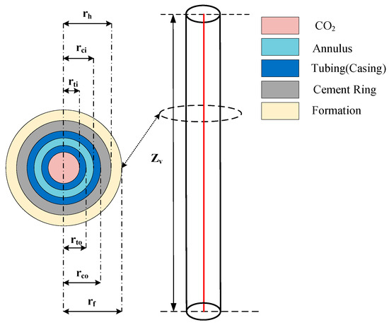
Figure 1. Schematic diagram of the CO₂ fracturing wellbore physical model.

Considering the large aspect ratio of the wellbore and the flow characteristics of carbon dioxide, a modeling method combining one-dimensional axial non-isothermal flow and one-dimensional radial transient heat transfer is adopted. To ensure the multi-physics problem remains manageable while preserving dominant coupling mechanisms, the following simplifying assumptions are introduced:

(1)

CO₂ flow within the tubing is treated as one-dimensional axial flow along the wellbore axis, accounting for temperature and pressure variations in the axial direction;

(2)

Heat conduction in the wellbore and formation zones is assumed to be one-dimensional radially;

(3)

Both the cement casing and formation are modeled as linear elastic materials;

(4)

The formation is treated as a homogeneous isotropic medium with a uniformly distributed initial temperature field; non-homogeneous and anisotropic effects are neglected;

(5)

At the initial time, the wellbore is filled with stationary fluid, and no pre-existing pressure fluctuations exist.

Based on the aforementioned physical assumptions, the computational domain is divided into the CO₂ zone, the wellbore zone, and the formation zone. The CO₂ zone exhibits non-isothermal flow characteristics, requiring the simultaneous solution of the continuity equation, momentum equation, and energy equation to describe its flow behavior. The wellbore zone and formation zone primarily experience natural convective heat transfer, necessitating only the solution of the energy equation. According to the law of mass conservation during CO₂ flow, the continuity equation is derived as:

$$u{\displaystyle \frac{\partial {\rho }_{\mathrm{f}}}{\partial z}}+{\rho }_{\mathrm{f}}{\displaystyle \frac{\partial u}{\partial z}}+{\displaystyle \frac{\partial {\rho }_{\mathrm{f}}}{\partial t}}=0$$

(1)

In the equation, ${\rho }_{\mathrm{f}}$ denotes the density of CO₂, kg/m³; t represents time, s; z indicates the axial extension distance of the wellbore, m; and u signifies the flow velocity of CO₂, m/s.

The pressure gradient represents the change in pressure per unit length along the tubing column. Based on the momentum equation, the expression for the pressure gradient within the tubing column is:

$${\displaystyle \frac{\partial p_{\mathrm{f}}}{\partial z}}={\rho }_{\mathrm{f}}g\sin \theta -{\displaystyle \frac{1}{2}}{f}_{\mathrm{D}}{\displaystyle \frac{{\rho }_{\mathrm{f}}{u}^2}{d_{\mathrm{ti}}}}-{\rho }_{\mathrm{f}}{\displaystyle \frac{\partial u}{\partial t}}$$

(2)

In the equation, ${\rho }_{\mathrm{f}}$ denotes CO₂ pressure, Pa; g is the acceleration due to gravity, m/s²; θ is the well inclination angle, rad; d_ti represents the inner diameter of the tubing, m; f_D is the friction factor, which can be calculated using the empirical formula proposed by Chen [35] applicable to the entire range of Reynolds numbers.

$${\displaystyle \frac{1}{\sqrt{f_{\mathrm{D}}}}}=-2\lg \left({\displaystyle \frac{e/d_{\mathrm{h}}}{3.7065}}-{\displaystyle \frac{5.0452}{Re}}\lg \left({\displaystyle \frac{{\left(e/d_{\mathrm{h}}\right)}^{1.1098}}{2.8257}}+{\displaystyle \frac{5.8506}{R{e}^{0.8981}}}\right)\right)$$

(3)

In the equation, e represents the absolute roughness of the wall surface, m; d_h denotes the hydraulic diameter, which can be taken as the diameter of the oil pipe, m.

The R_e calculation formula is as follows:

$$Re={\displaystyle \frac{{\rho }_{\mathrm{f}}u{d}_{\mathrm{h}}}{{\mu }_{\mathrm{f}}}}$$

(4)

In the equation, µ_f is the dynamic viscosity of CO₂, Pa·s.

To establish the energy change equation for CO₂, the energy conservation equation within an infinitesimal segment can be derived based on the law of conservation of energy:

$$A{\rho }_{\mathrm{f}}{c}_{\mathrm{pf}}\left({\displaystyle \frac{\partial T_{\mathrm{f}}}{\partial t}}+u{\displaystyle \frac{\partial T_{\mathrm{f}}}{\partial z}}\right)=Q_{\mathrm{wall}}$$

(5)

In the equation, A represents the cross-sectional area of the oil pipe, m²; c_pf denotes the specific heat capacity of CO₂, (J/(kg·°C)); T_f is the fluid temperature, °C.

Q_wall is the heat flux generated by wall heat transfer per unit axial length, in °C/m, defined as:

$$Q_{\mathrm{wall}}=\pi d_{\mathrm{ti}}{h}_{\mathrm{t}}\left(T_{\mathrm{f}}-T_{\mathrm{t}}\right)$$

(6)

In the equation, T_f is the fluid temperature, °C; T_t is the tubing temperature, °C; and h_t is the forced convective heat transfer coefficient on the tubing wall, W/(m²·°C), expressed as:

$$h_{\mathrm{t}}={\displaystyle \frac{{\lambda }_{\mathrm{f}}\left(f_{\mathrm{D}}/8\right)\left(Re-1000\right)Pr}{2r_{\mathrm{ti}}\left(1+12.7{\left(f_{\mathrm{D}}/8\right)}^{1/2}\left(P{r}^{2/3}-1\right)\right)}}$$

(7)

In the equation, λ_f denotes the thermal conductivity of CO₂, W/(m·°C); Pr is the Prandtl number for CO₂, defined as:

$$Pr={\displaystyle \frac{c_{\mathrm{pf}}{\mu }_{\mathrm{f}}}{{\lambda }_{\mathrm{f}}}}$$

(8)

The wellbore region comprises the tubing wall, annulus, casing wall, and cement ring. Except for the annulus, all other regions are solid phases, requiring consideration only of thermal conduction. Within the annulus, the internal fluid undergoes natural convection, characterized here by the natural convection heat transfer coefficient. The overall governing equation for the wellbore region is as follows:

$${\displaystyle \frac{1}{r}}{\displaystyle \frac{\partial }{\partial r}}\left(\lambda r{\displaystyle \frac{\partial T}{\partial r}}\right)=\rho c_{\mathrm{p}}{\displaystyle \frac{\partial T}{\partial t}}$$

(9)

In the equation, ρ, c_p, and λ represent material parameters that vary with spatial location, and temperatures at interfaces between different regions are continuous. The wellbore region is divided into single-layer meshes comprising the tubing wall, annulus, casing wall, and cement ring. The radial temperature distribution and geometric mesh division for the wellbore and formation during CO₂ fracturing are shown in Figure 2. The governing equations for each wellbore section are provided below.

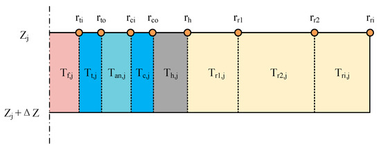
Figure 2. Radial mesh partitioning of the wellbore during CO₂ fracturing.

The energy control equation for the oil pipe wall is:

$${\displaystyle \frac{2r_{\mathrm{to}}{h}_{\mathrm{an}}\left(T_{\mathrm{an}}-T_{\mathrm{t}}\right)}{r_{\mathrm{to}}^2-r_{\mathrm{ti}}^2}}-{\displaystyle \frac{2r_{\mathrm{ti}}{h}_{\mathrm{t}}\left(T_{\mathrm{t}}-T_{\mathrm{f}}\right)}{r_{\mathrm{to}}^2-r_{\mathrm{ti}}^2}}={\rho }_{\mathrm{t}}{c}_{\mathrm{pt}}{\displaystyle \frac{\partial T_{\mathrm{t}}}{\partial t}}$$

(10)

The annular energy control equation is:

$${\displaystyle \frac{2r_{\mathrm{ci}}{h}_{\mathrm{an}}\left(T_{\mathrm{c}}-T_{\mathrm{an}}\right)}{r_{\mathrm{ci}}^2-r_{\mathrm{to}}^2}}-{\displaystyle \frac{2r_{\mathrm{to}}{h}_{\mathrm{an}}\left(T_{\mathrm{an}}-T_{\mathrm{t}}\right)}{r_{\mathrm{ci}}^2-r_{\mathrm{to}}^2}}={\rho }_{\mathrm{an}}{c}_{\mathrm{pan}}{\displaystyle \frac{\partial T_{\mathrm{an}}}{\partial t}}v$$

(11)

The energy control equation for the casing wall is:

$${\displaystyle \frac{2r_{\mathrm{co}}{\lambda }_{\mathrm{c},\mathrm{h}}\left(T_{\mathrm{h}}-T_{\mathrm{c}}\right)}{\left(r_{\mathrm{co}}^2-r_{\mathrm{ci}}^2\right)\left(r_{\mathrm{h}}-r_{\mathrm{ci}}\right)}}-{\displaystyle \frac{2r_{\mathrm{ci}}{h}_{\mathrm{an}}\left(T_{\mathrm{c}}-T_{\mathrm{an}}\right)}{r_{\mathrm{co}}^2-r_{\mathrm{ci}}^2}}={\rho }_{\mathrm{c}}{c}_{\mathrm{pc}}{\displaystyle \frac{\partial T_{\mathrm{c}}}{\partial t}}$$

(12)

The energy control equation for the cement ring is:

$${\displaystyle \frac{4r_{\mathrm{h}}{\lambda }_{\mathrm{h},\mathrm{r}}\left(T_{\mathrm{r}1}-T_{\mathrm{h}}\right)}{\left(r_{\mathrm{h}}^2-r_{\mathrm{co}}^2\right)\left(r_{\mathrm{r}1}-r_{\mathrm{co}}\right)}}-{\displaystyle \frac{4r_{\mathrm{co}}{\lambda }_{\mathrm{c},\mathrm{h}}\left(T_{\mathrm{h}}-T_{\mathrm{c}}\right)}{\left(r_{\mathrm{h}}^2-r_{\mathrm{co}}^2\right)\left(r_{\mathrm{h}}-r_{\mathrm{ci}}\right)}}={\rho }_{\mathrm{h}}{c}_{\mathrm{ph}}{\displaystyle \frac{\partial T_{\mathrm{h}}}{\partial t}}$$

(13)

In the equation, r_ti denotes the inner radius of the tubing, m; r_to denotes the outer radius of the tubing, m; T_an represents the annular temperature, °C; T_t indicates the tubing temperature, °C; T_h is the temperature of the cement annulus, °C; r_ci denotes the inner radius of the casing, m; ρ_an is the annular density, kg/m³; c_pan is the annular specific heat capacity, J/(kg·°C); T_c is the casing temperature, °C; r_co is the casing outer radius, m; ρ_c is the density of the casing, kg/m³; c_pc is the specific heat capacity of the casing, J/(kg·°C); T_h is the temperature of the cement annulus, °C; r_h is the outer radius of the cement annulus, m; ρ_h is the density of the cement annulus, kg/m³; c_ph is the specific heat capacity of the cement annulus, J/(kg·°C); r_r1 denotes the position of the first grid in the formation, m; T_r1 denotes the temperature of the first formation grid, °C; λ_c,h and λ_h,r are the composite thermal conductivities.

The equivalent heat transfer coefficient formula for plates by Dropkin and Somerscales [36] is approximated for h_an as follows:

$$h_{\mathrm{an}}={\displaystyle \frac{0.049{\left(Gr\cdot Pr\right)}^{1/3}P{r}^{0.074}{\lambda }_{\mathrm{an}}}{r_{\mathrm{to}}\ln \left(r_{\mathrm{ci}}/r_{\mathrm{to}}\right)}}$$

(14)

$$G{r}_{\mathrm{an}}={\displaystyle \frac{{\left(r_{\mathrm{ci}}-r_{\mathrm{to}}\right)}^{3}g{\rho }_{\mathrm{an}}^2{\beta }_{\mathrm{an}}\left(T_{\mathrm{t}}-T_{\mathrm{c}}\right)}{{\mu }_{\mathrm{an}}^2}}$$

(15)

$$P{r}_{\mathrm{an}}={\displaystyle \frac{c_{\mathrm{pan}}{\mu }_{\mathrm{an}}}{{\lambda }_{\mathrm{an}}}}$$

(16)

In the equation, G_ran denotes the Grashof number of the annular fluid; P_ran denotes the Prandtl number of the annular fluid; λ_an represents the thermal conductivity of the annular fluid, W/(m·°C); ρ_an indicates the density of the annular fluid, kg/m³; μ_an signifies the viscosity of the annular fluid, Pa·s; c_pan reflects the specific heat capacity at constant pressure of the annular fluid, J/(kg·°C); β_an signifies the thermal expansion coefficient of the annular fluid, 1/°C. λ_c,h, and λ_h,r can be calculated according to Fourier’s law:

$${\lambda }_{\mathrm{c},\mathrm{h}}={\displaystyle \frac{{\lambda }_{\mathrm{c}}{\lambda }_{\mathrm{h}}\ln \left(\frac{r_{\mathrm{co}}+r_{\mathrm{h}}}{r_{\mathrm{co}}+r_{\mathrm{ci}}}\right)}{{\lambda }_{\mathrm{c}}\ln \left(\frac{r_{\mathrm{co}}+r_{\mathrm{h}}}{2r_{\mathrm{co}}}\right)+{\lambda }_{\mathrm{h}}\ln \left(\frac{2r_{\mathrm{co}}}{r_{\mathrm{co}}+r_{\mathrm{ci}}}\right)}}$$

(17)

$${\lambda }_{\mathrm{h},\mathrm{r}}={\displaystyle \frac{{\lambda }_{\mathrm{h}}{\lambda }_{\mathrm{r}}\ln \left(\frac{r_{\mathrm{h}}+r_{\mathrm{r}1}}{r_{\mathrm{h}}+r_{\mathrm{co}}}\right)}{{\lambda }_{\mathrm{h}}\ln \left(\frac{r_{\mathrm{h}}+r_{\mathrm{r}1}}{2r_{\mathrm{h}}}\right)+{\lambda }_{\mathrm{r}}\ln \left(\frac{2r_{\mathrm{h}}}{r_{\mathrm{h}}+r_{\mathrm{co}}}\right)}}$$

(18)

In the equation, λc is the thermal conductivity of the casing, W/(m·°C); λ_h is the thermal conductivity of the cement annulus, W/(m·°C); λ_r is the thermal conductivity of the formation, W/(m·°C).

Given the absence of fluid flow within the strata, its energy conservation equation can be simplified to the heat conduction equation:

$${\displaystyle \frac{4r_{\mathrm{r}1}{\lambda }_{\mathrm{r}}\left(T_{\mathrm{r}2,\mathrm{j}}-T_{\mathrm{r}1,\mathrm{j}}\right)}{\left(r_{\mathrm{r}1}^2-r_{\mathrm{h}}^2\right)\left(r_{\mathrm{r}2}-r_{\mathrm{h}}\right)}}-{\displaystyle \frac{4r_{\mathrm{h}}{\lambda }_{\mathrm{h},\mathrm{r}}\left(T_{\mathrm{r}1,\mathrm{j}}-T_{\mathrm{h},\mathrm{j}}\right)}{\left(r_{\mathrm{r}1}^2-r_{\mathrm{h}}^2\right)\left(r_{\mathrm{r}1}-r_{\mathrm{co}}\right)}}={\rho }_{\mathrm{r}}{c}_{\mathrm{pr}}{\displaystyle \frac{\partial T_{\mathrm{r}1}}{\partial t}}$$

(19)

In the equation, r_ri denotes the i-th grid position in the formation, m; T_ri denotes the temperature of the i-th grid in the formation, °C.

The flow of CO₂ within fracturing tubing represents a dynamic evolution of its physical and thermodynamic properties. Therefore, when calculating temperature and pressure variations during CO₂ fracturing operations, it is essential to account for the significant changes in its physical properties with respect to temperature and pressure, particularly when crossing phase transitions such as liquid, supercritical phases, and regions near critical points. To accurately capture this complex phase behavior and its impact on flow and heat transfer, this study employs the following extensively validated, high-precision physical property calculation models: The Span-Wagner equation of state [37] is used to calculate CO₂ density and specific heat capacity at constant pressure. This equation offers excellent accuracy, fully covering the supercritical, liquid, and critical regions commonly encountered in CO₂ fracturing operations. It reliably describes the thermodynamic properties of CO₂ across multiple phases and accurately characterizes the dramatic changes in physical properties near the critical point. The Fenghour model [38] was employed to calculate CO₂’s dynamic viscosity. This model accurately characterizes viscosity changes in both subcritical and supercritical regions, aligning with the temperature-pressure range encountered in fracturing operations. The Vesovic model [39] was used to compute CO₂’s thermal conductivity. This model accounts for the enhancement effect of thermal conductivity near the critical region, aligning with the temperature-pressure range of the fracturing injection process. This is crucial for simulating heat transfer during CO₂ injection. The aforementioned models are invoked in real-time at each time step and spatial node during computation. Local CO₂ properties are updated based on the instantaneous temperature and pressure obtained from the coupled solution, ensuring the model accurately reflects the impact of CO₂ phase transitions and nonlinear property changes on multiphysics processes.

Considering the influence of initial and boundary conditions, the initial wellbore temperature may be calculated using the geothermal gradient. For pressure, assuming the wellbore is filled with CO₂, the initial hydrostatic column pressure within the wellbore may be obtained via an iterative method incorporating a CO₂ density model. The governing equations for initial conditions are as follows:

$${\left.T\right|}_{t=0}=T_{\mathrm{surf}}+T_{\mathrm{G}}\cdot z$$

(20)

$${\left.p\right|}_{t=0}={\displaystyle {\int }_0^z\rho \left(T,p\right)}g\mathrm{d}z$$

(21)

In the equation, T_surf represents the surface temperature in °C; T_G is the geothermal gradient, °C/m.

For the CO₂ regional flow field, the injection flow rate is specified at the wellhead as the velocity boundary condition, while pressure must be specified at the wellbore bottom. In this project, fracture closure pressure is employed as the wellbore bottom pressure boundary. For the CO₂ regional temperature field, the injection temperature is specified at the wellhead as the temperature boundary condition, with the wellbore bottom treated as adiabatic but accounting for thermal convection. The governing equations for the boundary conditions are as follows:

$${\left.u\right|}_{z=0}=Q_{\mathrm{inj}}/\left(\pi r_{\mathrm{ti}}^2\right)$$

(22)

$${\left.p\right|}_{z=z_{\mathrm{bh}}}=p_{\mathrm{w}}$$

(23)

$${\left.T\right|}_{z=0}=T_{\mathrm{inj}}$$

(24)

$${\left.{\displaystyle \frac{\partial T}{\partial z}}\right|}_{z=z_{\mathrm{bh}}}=0$$

(25)

In the equation, Q_inj denotes the injection flow rate, m³/min; p_w represents the bottomhole fracture closure pressure, Pa; T_inj indicates the injection temperature, °C; and z_bh signifies the bottomhole depth, m. For radial heat transfer in the wellbore and formation regions, the inner boundary adjacent to the CO₂ zone is defined as a Neumann boundary, where heat flux is determined by the temperature difference between CO₂ and the tubing wall. The outer formation boundary temperature is maintained constant at the original formation temperature. The governing equations are as follows:

$${\left.{\displaystyle \frac{1}{r}}{\displaystyle \frac{\partial }{\partial r}}\left(\lambda r{\displaystyle \frac{\partial T}{\partial r}}\right)\right|}_{r=r_{\mathrm{ti}}}={\displaystyle \frac{2h_{\mathrm{t}}}{r_{\mathrm{ti}}}}\left(T_{\mathrm{t}}-T_{\mathrm{f}}\right)$$

(26)

$${\left.T\right|}_{r=r_{\mathrm{f}}}=T_{\mathrm{out}}={\left.T\right|}_{t=0}$$

(27)

Based on the group equations established earlier, the changes in flow velocity, pressure, and temperature during the CO₂ flow process can be systematically solved. Further derivation yields:

$$\Delta u={\displaystyle \frac{-\Delta z\Delta {\rho }_{\mathrm{f}}\left(\frac{1}{\Delta t}+u\frac{1}{\Delta z}\right)}{{\rho }_{\mathrm{f}}}}$$

(28)

$$\Delta p_f=\Delta z\left({\rho }_{f}g\sin \theta -{\displaystyle \frac{1}{2}}{f}_D{\displaystyle \frac{{\rho }_f{u}^2}{d_{ti}}}-{\rho }_f{\displaystyle \frac{\Delta u}{\Delta t}}\right)$$

(29)

$$\Delta T_f={\displaystyle \frac{\pi d_{ti}{h}_t\left(T_f-T_t\right)}{A{\rho }_f{c}_{pf}\left(\frac{1}{\Delta t}+u\frac{1}{\Delta z}\right)}}$$

(30)

As derived earlier, this model constitutes a transient nonlinear system coupled by the continuity equation, momentum equation, and energy equation. These equations are coupled through the interaction of temperature, pressure, and CO₂ physical properties. Due to the highly nonlinear and transiently coupled nature of this system of equations, obtaining an analytical solution directly is challenging. Therefore, this study employs Python for numerical iterative solutions. The core solution employs a double-loop iterative structure: the inner loop is a pressure-velocity iteration, solving the continuity and momentum equations under a given initial temperature; the outer loop is a temperature iteration, which simultaneously solves the energy equations for the CO₂ domain, wellbore domain, and formation domain. The updated pressure, velocity, and physical property parameters are then fed into the temperature iteration process to solve the energy equations. This nested strategy ensures full coupling of pressure, velocity, and temperature variables at each time step. Only when all variables meet convergence criteria does the next time step proceed. The detailed solution workflow is illustrated in Figure 3. To further guarantee solution stability, convergence is achieved through error correction of the medium flow velocity within the tubing during iteration. No convergence issues have been observed to date. In terms of computational efficiency, simulating a 1-s fracturing process requires approximately 0.5 to 1 s of computation time, meeting the rapid analysis demands of engineering applications.

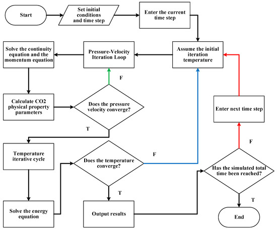
Figure 3. Temperature-pressure calculation flowchart for the CO₂ fracturing process.

2.2. Calculation Model for Tubing Loads During CO₂ Fracturing Processes

Under CO₂ fracturing conditions, the axial load state of the downhole tubing string exhibits complex multi-factor coupling characteristics. Figure 4 illustrates the force distribution on the tubing string during CO₂ fracturing. Beyond the axial forces induced by the tubing’s self-weight and temperature effects, the additional axial forces generated by expansion effects and fluid friction resistance during CO₂ fracturing must also be considered in analyzing the tubing’s mechanical behavior [40]. Due to the gravitational distribution characteristics of the tubing string, axial forces exhibit a gradient variation along the wellbore depth. The near-wellhead region bears accumulated axial loads from the weight of the lower tubing string, resulting in significantly higher axial forces compared to other well sections. The specific axial force calculation method is as follows:

$$F_a=F_t+F_p+F_w+F_z$$

(31)

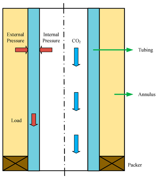
Figure 4. Schematic diagram of tubing loading during the CO₂ fracturing process.

In the equation, F_t represents the axial force caused by temperature effects, N; F_p represents the axial force caused by swelling effects on the fracturing string, N; F_w represents the axial force caused by fluid friction effects, N; F_z represents the axial force caused by the weight of the string, N.

After CO₂ injection, the transient temperature field calculation yields ΔT_f, creating a temperature difference between the inner and outer walls of the tubing. This causes the tubing string to contract due to cooling. If constrained by the packer and unable to contract freely, an additional axial force is generated, calculated as follows:

$$F_t={\sigma }_t{A}_i=E\alpha \Delta T_f{A}_i$$

(32)

In the formula: σ_t represents the axial stress caused by temperature variation, Pa; E denotes the elastic modulus of the tubing string, Pa; α signifies the linear thermal expansion coefficient of the tubing material, 1/°C; ΔT_f indicates the temperature change of CO₂, °C; A_i represents the cross-sectional area of the tubing, m².

The internal and external pressure differential ΔP, calculated from the transient pressure field, comprises internal pressure from CO₂ and external pressure from the annulus. This differential is not constant but varies with time and depth. This dynamic value is obtained by solving the energy equations for the annulus and surrounding wellbore regions within the coupled transient model. The resulting expansion effect on the tubing string generates axial forces as follows:

$$F_p={\sigma }_p{A}_{\mathrm{j}}=2\mu \left(p_i{A}_i-p_o{A}_o\right)$$

(33)

In the equation: σ_p is the axial stress caused by expansion effects, Pa; µ is the Poisson’s ratio of the tubing material; P_i is the CO₂ pressure, Pa; P_o is the annular pressure, Pa; A_i is the inner surface area of the tubing, m²; A_o is the outer surface area of the tubing, m²; A_j is the cross-sectional area of the tubing, m².

The fluid velocity u calculated from the transient temperature-pressure field determines the fluid friction resistance between CO₂ and the inner wall of the tubing string. During flow, the axial force induced by fluid friction within the pipe is:

$$F_w={\tau }_w(L\pi d)={\displaystyle \frac{125L\pi d_{\mathrm{ti}}{\mathrm{u}}^2\rho }{48\sqrt{R_e}}}$$

(34)

In the equation, τ_w represents the shear stress on the pipe wall, Pa; Re denotes the Reynolds number; d_ti indicates the inner diameter of the tubing, m; ρ signifies the fluid density within the wellbore, kg/m³; u represents the CO₂ flow velocity, m/s; L denotes the length of the tubing string, m.

Axial force caused by the weight of the lower section of the z-th pipe section:

$$F_z={\sigma }_z{A}_{\mathrm{z}}={\rho }_{\mathrm{g}}\mathrm{g}{L}_{\mathrm{down}}$$

(35)

In the equation, σ_z represents the axial stress caused by the weight of the tubing string, Pa; ρ_g denotes the nominal weight of the tubing string, kg/m; L_down indicates the length of the lower section of the z-th segment, m; and A_z signifies the cross-sectional area of the tubing, m².

Considering that the downhole tubing string typically experiences triaxial stress conditions during CO₂ fracturing operations, triaxial stress verification is conducted according to the fourth strength theory. The safety factor calculation formula is as follows:

$$K_s={\displaystyle \frac{\left[\sigma \right]}{{\sigma }_4}}$$

(36)

In the formula, [σ] denotes the allowable stress of the tubing string, Pa; σ₄ denotes the equivalent stress, Pa.

According to the fourth-strength theory, the expression for equivalent stress can be derived:

$${\sigma }_4={\displaystyle \frac{\sqrt{2}}{2}}\sqrt{{\left({\sigma }_a-{\sigma }_{\theta }\right)}^2+{\left({\sigma }_{\theta }-{\sigma }_r\right)}^2+{\left({\sigma }_r-{\sigma }_a\right)}^2}$$

(37)

In the equation, σ_a represents axial stress, Pa; σ_r represents radial stress of the tubing string, Pa; σ_θ represents circumferential stress of the tubing string, Pa.

2.3. Solving Multi-Physics Coupled Transient Analysis Models

Solving the CO₂ fracturing multi-field coupled transient analysis model requires Python numerical iteration as the core tool, integrating the transient temperature-pressure field model with the tubing string load calculation model. The CO₂ temperature, pressure, and flow velocity parameters obtained from the transient temperature-pressure field model are then processed through the tubing load calculation model. This model superimposes temperature-induced forces, pressure-induced forces, fluid friction forces, and tubing gravity to derive the tubing axial force. Subsequently, the safety factor is calculated to evaluate the engineering safety. If unsafe, the injection parameters are adjusted, and the relevant parameters and safety factor are re-iterated and recalculated. Finally, the tubing load indicators are output, as shown in Figure 5.

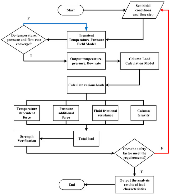
Figure 5. Computational flowchart for multiphysics coupled transient analysis of CO₂ fracturing Processes.

3. Results

Taking an experimental well in the Xinjiang oilfield as an example for computational analysis, the well depth structure is shown in Figure 6, with basic parameters listed in Table 1 and detailed tubing configuration provided in Appendix A. During the experiment, sensors deployed in the perforated section recorded real-time fracturing-related data. After calibration, the measurement error was verified to be less than 10%, providing reliable data support for subsequent analysis. By systematically controlling the injection temperature, pressure, and flow rate of the CO₂ fluid, the study focused on investigating the evolution patterns of tubing string loads during fracturing and the influence mechanisms of injection parameters on these loads. This clarified the correlation between different injection parameters and the dynamic characteristics of tubing string loads.

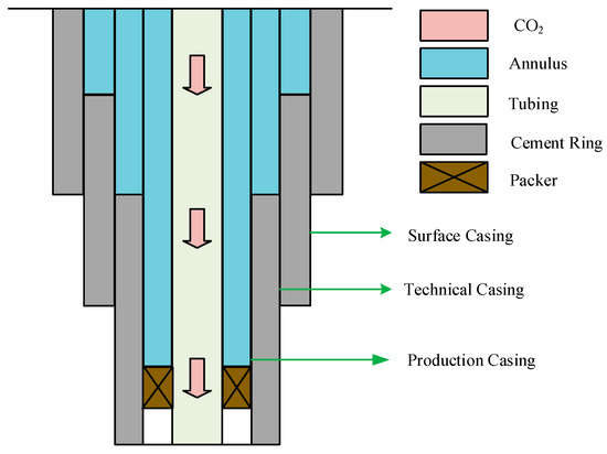
Figure 6. Schematic diagram of well depth structure during the CO₂ fracturing process.

Table 1. Basic parameters of an experimental well in Xinjiang Oilfield.

Parameters	Symbol	Numerical Value
Well depth/m	H	6200
Surface temperature/°C	Tsurf	12.89
Oil pipe Inner Diameter/mm	rti	69.86
Oil pipe Outer Diameter/mm	rto	88.9
Casing Inner Diameter/mm	rci	124.26
Casing Outer Diameter/mm	rco	139.7
Cement ring radius/mm	rh	234.5
Nominal weight of pipe column/(kg/m)	ρg	18.90
Elastic modulus of the pipe column/Pa	E	2.06 × 1011
Thermal conductivity of the casing/(W/(m·°C))	λc	44.8
Thermal Conductivity of Cement Ring/(W/(m·°C))	λh	0.89
Thermal conductivity of formation/(W/(m·°C))	λr	1.92
Geothermal gradient/(°C/m)	TG	0.024
Injection temperature/°C	Tinj	10
Injection pressure/MPa	Pf	80
Injection flow rate/(m3/min)	Qinj	2

3.1. Evolutionary Characteristics of Dynamic Loads on the Tubing String During the Fracturing Process

A multi-field coupled transient analysis model was used for computation based on the previously mentioned operating parameters. Figure 7 displays the transient temperature field contour plots produced by the model at 180, 360, 540, and 720 s during the CO₂ fracturing process. The spatiotemporal evolution characteristics of temperatures within the wellbore and near-formation regions under multi-field coupling effects are graphically depicted in this figure. Two fundamental features are evident in the simulation results: (1) The temperature drops radially in a gradient from the tubing’s inner wall toward the formation; (2) The temperature at the same wellbore depth keeps dropping as the fracturing time increases. The thorough analysis of tubing string loads under multi-field coupling conditions is crucially supported by these temperature field simulation results, which offer trustworthy core input parameters for ensuing tubing string load computations.

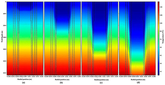
Figure 7. Transient temperature field contour plots under CO₂ fracturing multi-field coupling at different fracturing times: (a) t = 180 s, (b) t = 360 s, (c) t = 540 s, and (d) t = 720 s.

By injecting CO₂ fracturing fluid at a temperature of 10 °C, pressure of 80 MPa, and flow rate of 2 m³/min, the resulting time-dependent contour plots for temperature, pressure, flow velocity, load, equivalent stress, and safety factor are shown in Figure 8 and Figure 9. The variation patterns of each parameter with well depth and fracturing duration are as follows.

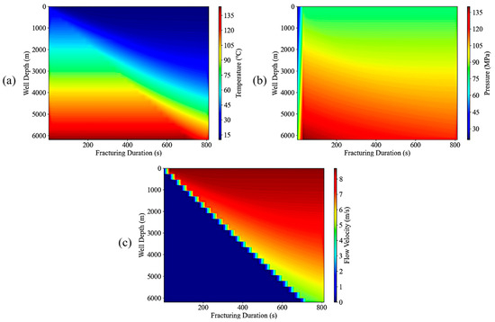
Figure 8. Injection parameters—time cloud diagram: (a) temperature, (b) pressure, (c) flow rate.

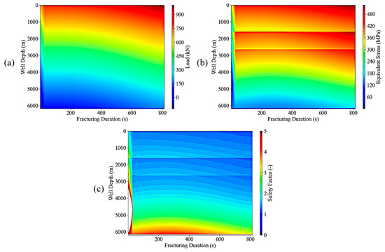
Figure 9. String load-time cloud diagram: (a) load, (b) equivalent stress, (c) Safety factor.

CO₂ undergoes continuous heat exchange with the formation through the wellbore wall. Under the influence of the geothermal gradient, temperature increases significantly with increasing well depth. Simultaneously, the continuous injection of low-temperature CO₂ cools the surrounding formation, causing the temperature at the same well depth to decrease with prolonged injection duration. For instance, at a depth of 3000 m, following a fracturing duration exceeding 300 s, the temperature gradually decreased from 95 °C to approximately 75 °C. This cooling effect is more pronounced in shallow well sections due to faster thermal equilibrium, whereas in deeper sections with greater thermal capacity, significant cooling only occurs after prolonged fracturing, as illustrated in Figure 8a.

As well, depth increases, and static pressure gradually accumulates, with pressure rising significantly with depth. For instance, pressures in deep well sections exceed 120 MPa, while those in shallow sections remain below 60 MPa. Concurrently, CO₂ continuously diffuses and permeates into the formation, entering fractures and pores. This causes wellbore pressure to decrease with increasing fracturing duration, as shown in Figure 8b.

Flow velocities exhibit significant variations at different depths within the wellbore, with the highest velocities occurring near the shallow well section, exceeding 8 m/s in such zones. Besides, under identical fracturing durations, velocities decrease progressively with increasing well depth. During the initial fracturing phase, high-velocity zones are concentrated near the wellbore’s proximal end. As fractures propagate and expand, these high-velocity zones gradually advance deeper into the formation, concurrently leading to a more uniform overall velocity distribution, as illustrated in Figure 8c.

As the wellhead constitutes the suspension end of the tubing string, it typically bears greater mechanical loads. Load values exhibit a gradual decrease with increasing well depth, whilst at a given depth, they show an upward trend with extended fracturing duration. For instance, at the 6000 m deep well section, load values progressively rose from 0 to approximately 150 kN as fracturing duration increased from 0 to 800 s. The load gradient transition zone progressively extends towards the deep well section with increasing fracturing duration, as illustrated in Figure 9a.

Due to high wellhead loads and substantial axial stresses, coupled with low bottomhole loads and minimal axial stresses, equivalent stress decreases significantly with increasing well depth. For instance, values exceed 480 MPa in shallow sections but fall below 60 MPa in deep sections, exhibiting distinct stratification influenced by packers. At the same depth, equivalent stress increases with extended fracturing duration, as illustrated in Figure 9b.

The wellhead exhibits the highest equivalent stress and a fixed allowable stress, resulting in the lowest safety factor. Conversely, the well bottoms display the lowest equivalent stress and the highest safety factor. The safety factor increases with well depth, approaching 5 at 6000 m in the deep well section and approximately 1.5 in the shallow well section and certain stratified intermediate zones. A distinct stratification is observed due to the effects of the packer. As fracturing duration increases, safety factors across all well sections exhibit a sustained downward trend. Notably, the lower well section approaches critical values during the latter stages of fracturing, as illustrated in Figure 9c.

3.2. Influence of Characteristics of Injection Parameters on Payload

Injection temperature, pressure, and flow rate significantly affect tubing string loads and safety factors. Well depth is the key determinant of load variation, while injection parameters serve a regulatory function.

When the injection time is fixed at 50 MPa injection pressure and 2 m³/min injection flow rate, the corresponding load distribution and safety factor effects for injection temperatures of 0 °C, 5 °C, 10 °C, 15 °C, and 20 °C are calculated and shown in Figure 10. Figure 10a indicates that the tubing string load decreases with well depth, and the peak load at the wellhead is influenced by the following factors: (1) The maximum temperature difference between CO₂ and the tubing string at the wellhead induces significant thermal expansion effects; (2) The highest CO₂ flow velocity at the wellhead causes fluid friction effects to dominate axial stress distribution. Additionally, increasing injection temperature reduces axial stress caused by temperature effects by lowering the temperature difference, resulting in an overall decrease in tensile stress on the tubing string. Figure 10b shows that the variation in the safety factor is jointly regulated by injection temperature and well depth: (1) Low-temperature injection increases tubing string loading, elevating axial stress. Concurrently, changes in pressure-induced stress further increase radial and circumferential stresses. The combined effect of these three stresses significantly increases the equivalent stress. Under conditions where the allowable stress remains constant, the safety factor consequently decreases; (2) Along the wellbore depth, the tubing string load gradually decreases, leading to corresponding reductions in axial, radial, and circumferential stresses. This results in a progressive increase in the safety factor.

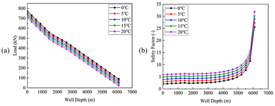
Figure 10. Different injection temperatures versus load and well depth: (a) load, (b) safety factor.

When the injection time is fixed, the injection temperature is 10 °C, and the injection flow rate is 2 m³/min, the corresponding load distribution and the impact of safety factors under injection pressures of 40 MPa, 50 MPa, 60 MPa, 70 MPa, and 80 MPa are calculated and shown in Figure 11. Figure 11a indicates that tubing loads decrease with well depth. However, increased injection pressure alters the load distribution through the following mechanisms: (1) Axial forces induced by expansion effects intensify with rising internal pressure; (2) Simultaneous increases in fluid density and flow velocity exacerbate friction effects, ultimately leading to a significant rise in bottomhole stress. Figure 11b reveals that safety factor variations are jointly governed by injection pressure and well depth: (1) Higher injection pressure increases tubing string loads and axial stress while maintaining allowable stress constant, ultimately reducing the safety factor; (2) As well depth increases, tubing string loads decrease progressively, causing simultaneous reductions in axial, radial, and circumferential stresses, which gradually elevates the safety factor.

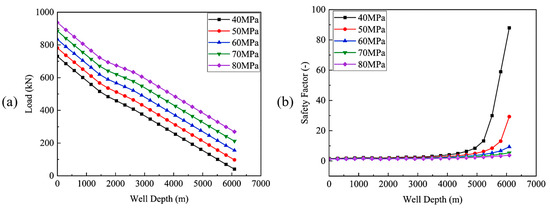
Figure 11. Different injection pressures versus load and well depth: (a) load, (b) safety factor.

When the injection time is fixed at 10 °C and the injection pressure at 80 MPa, the corresponding load distribution and safety factor effects for injection flow rates of 1.5 m³/min, 2 m³/min, 2.5 m³/min, 3 m³/min, and 3.5 m³/min are shown in Figure 12. Figure 12a indicates that increased injection flow rates exacerbate tubing loads through the following mechanisms: (1) Lowered fluid temperature increases the temperature difference between the tubing and the fluid, intensifying axial forces induced by thermal effects; (2) Simultaneous increases in flow rate and pressure cause friction and expansion effects to act in concert, leading to a significant rise in tubing loads. Figure 12b demonstrates that the safety factor is jointly regulated by injection flow rate and well depth: (1) Higher injection flow rates increase tubing string loads, thereby elevating axial stress and significantly raising equivalent stress, causing the safety factor to decrease with increasing flow rate; (2) Along the well depth, tubing string loads decrease progressively, with axial stress diminishing synchronously, resulting in the safety factor gradually increasing with greater well depth.

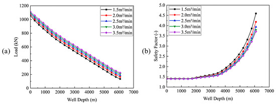
Figure 12. Different injection flow rates versus load and well depth: (a) load, (b) safety factor.

3.3. Differences Between CO₂ Fracturing and Hydraulic Fracturing

CO₂ fracturing and hydraulic fracturing exhibit differences in tubing string loading and casing pressure differential distribution, which directly impact operational safety and tubing failure risks.

Regarding string loading, CO₂ fracturing’s low-temperature properties positively influence load distribution. The supercritical CO₂’s low-temperature state creates a cooling effect on the string. Its low viscosity and density characteristics promote more uniform evolution of the wellbore temperature field, resulting in a more gradual decrease in load along the wellbore depth. In contrast, hydraulic fracturing uses water-based fracturing fluids with high heat capacity, which can cause abrupt temperature changes in the wellbore and trigger significant thermal stress concentration. Furthermore, CO₂ fracturing exhibits no water sensitivity, eliminating additional loads caused by reservoir damage, such as clay swelling associated with hydraulic fracturing. Through multi-field coupling model optimization, the safety factor of CO₂ fracturing tubing typically increases with well depth, resulting in lower overall failure risk.

Regarding casing pressure differentials, the two fracturing methods exhibit fundamentally different mechanisms and consequences. CO₂’s low density results in a smaller hydrostatic column pressure gradient, distributing casing pressure differentials more uniformly along well depth. These differentials also change more gradually with time and depth, effectively mitigating abrupt axial force variations caused by expansion effects. In contrast, hydraulic fracturing using high-density water-based fluids can generate significant pressure fluctuations, intensifying radial and circumferential stress variations in the tubing string. This increases the risk of casing collapse and coupling loosening. Furthermore, CO₂ fracturing avoids additional differential pressure loads induced by reservoir damage. Combined with a multi-field coupling design, it enables precise prediction of casing-tubing differential pressure. Hydraulic fracturing, however, often relies on static design standards, making it difficult to adapt to dynamic pressure fluctuations encountered during actual operations. This results in significant deviations in assessment outcomes.

4. Conclusions

Temperature, pressure, and flow velocity exhibit strongly non-linear transient coupled variations. Temperature increases with well depth but decreases with fracturing duration, with more pronounced cooling occurring in the shallow well section. Pressure accumulates with increasing well depth but shows a decreasing trend with CO₂ formation permeability, revealing significant pressure differences between shallow and deep sections. Flow velocity peaks in the shallow section, diminishes with depth, and later tends towards uniform distribution as fractures propagate.

Tubing loads exhibit a trend of initially slow increase followed by accelerated growth during fracturing, decreasing with well depth. The safety factor continuously declines with fracturing duration, approaching critical values in the lower well sections during the later stages.

Injection parameters exert a clear regulatory effect on tubing loads. Increasing injection temperature helps reduce thermal stresses caused by temperature differentials, thereby decreasing tubing loads. Conversely, lowering injection pressure or reducing flow rate mitigates fluid expansion effects and friction resistance, consequently reducing tubing loads and enhancing operational safety factors.

This model ignores anisotropy and assumes that the formation is homogeneous and isotropic. It treats the tubing material as linearly elastic and uses a one-dimensional fluid and heat conduction model. In addition to establishing an operational multiphysics coupling framework centered on transient thermal-fluid-mechanical coupling in the wellbore region, these simplifications guarantee computational viability. However, they ignore material nonlinearity and geological heterogeneity—two major shortcomings of the current model—and restrict direct applicability to highly heterogeneous reservoirs. In terms of applicability, the model can be used for transient continuous CO₂ injection in a 6200-m vertical fractured well under standard operating conditions, which include injection temperatures between 0 and 20 °C, pressures between 40 and 80 MPa, and flow rates between 1.5 and 3.5 m³/min. These ranges are consistent with earlier parameter studies that have been used to validate the model. Further validation using field data or model extension is advised for extreme conditions outside of these ranges. Future studies will concentrate on improving the model’s predictive accuracy and engineering applicability, incorporating more intricate cement-rock constitutive relationships, and integrating field monitoring data to validate predictions.

References

- Zhang, C.; Liu, S.; Ma, Z.; Ranjith, P. Combined micro-proppant and supercritical carbon dioxide (SC-CO2) fracturing in shale gas reservoirs: A review. Fuel 2021, 305, 25. [Google Scholar] [CrossRef]
- Zhu, C.-F.; Guo, W.; Wang, Y.-P.; Li, Y.-J.; Gong, H.-J.; Xu, L.; Dong, M.-Z. Experimental study of enhanced oil recovery by CO2 huff-n-puff in shales and tight sandstones with fractures. Pet. Sci. 2021, 18, 852–869. [Google Scholar] [CrossRef]
- Cao, L.; Lv, M.; Li, C.; Sun, Q.; Wu, M.; Xu, C.; Dou, J. Effects of crosslinking agents and reservoir conditions on the propagation of fractures in coal reservoirs during hydraulic fracturing. Reserv. Sci. 2025, 1, 36–51. [Google Scholar] [CrossRef]
- Memon, S.; Feng, R.; Ali, M.; Bhatti, M.A.; Giwelli, A.; Keshavarz, A.; Xie, Q.; Sarmadivaleh, M. Supercritical CO2-Shale interaction induced natural fracture closure: Implications for scCO2 hydraulic fracturing in shales. Fuel 2022, 313, 15. [Google Scholar] [CrossRef]
- Li, Q.; Li, Q.; Wang, F.; Xu, N.; Wang, Y.; Bai, B. Settling behavior and mechanism analysis of kaolinite as a fracture proppant of hydrocarbon reservoirs in CO2 fracturing fluid. Colloids Surf. A Physicochem. Eng. Asp. 2025, 724, 11. [Google Scholar] [CrossRef]
- Wu, J.; Ansari, U. From CO2 Sequestration to Hydrogen Storage: Further Utilization of Depleted Gas Reservoirs. Reserv. Sci. 2025, 1, 19–35. [Google Scholar] [CrossRef]
- Ma, Q.; Li, H.; Ji, K.; Huang, F. Thermal-Hydraulic-Mechanical Coupling Simulation of CO2 Enhanced Coalbed Methane Recovery with Regards to Low-Rank but Relatively Shallow Coal Seams. Appl. Sci. 2023, 13, 2592. [Google Scholar] [CrossRef]
- Roy, P.; Morris, J.P.; Walsh, S.D.; Iyer, J.; Carroll, S. Effect of thermal stress on wellbore integrity during CO2 injection. Int. J. Greenh. Gas Control 2018, 77, 14–26. [Google Scholar] [CrossRef]
- Wang, F.; Kobina, F. The influence of geological factors and transmission fluids on the exploitation of reservoir geothermal resources: Factor discussion and mechanism analysis. Reserv. Sci. 2025, 1, 3–18. [Google Scholar] [CrossRef]
- Nygaard, R.; Salehi, S.; Weideman, B.; Lavoie, R.G. Effect of Dynamic Loading on Wellbore Leakage for the Wabamun Area CO2-Sequestration Project. J. Can. Pet. Technol. 2014, 53, 69–82. [Google Scholar] [CrossRef]
- Enyi, Y.; Yuan, D.; Hui, W.; Xiaopeng, C.; Qingfu, Z.; Chuanbao, Z. Numerical simulation on risk analysis of CO2 geological storage under multi-field coupling: A review. Lixue Xuebao 2023, 55, 2075–2090. [Google Scholar]
- Zhao, T.; Duan, M.; Pan, X.; Feng, X. Lateral buckling of non-trenched high temperature pipelines with pipelay imperfections. Pet. Sci. 2010, 7, 123–131. [Google Scholar] [CrossRef]
- Ferla, A.; Lavrov, A.; Fjær, E. Finite-element analysis of thermal-induced stresses around a cased injection well. J. Phys. Conf. Ser. 2009, 181, 012051. [Google Scholar] [CrossRef]
- Zhang, Z.; Ding, J.; Zheng, Y.; Sang, P.; Chen, L.; Fan, Y.; Li, Y. Mechanical integrity of tubing string in high-temperature and high-pressure ultra-deep gas wells based on uncertainty theory. Energy Sci. Eng. 2022, 10, 2106–2122. [Google Scholar] [CrossRef]
- Li, J.; Li, Z. Mechanical analysis of tubing string in fracturing operation. Open Pet. Eng. J. 2013, 6, 12–24. [Google Scholar] [CrossRef]
- Khudayarov, B.A.; Komilova, K.M.; Turaev, F.Z. Numerical study of the effect of viscoelastic properties of the material and bases on vibration fatigue of pipelines conveying pulsating fluid flow. Eng. Fail. Anal. 2020, 115, 14. [Google Scholar] [CrossRef]
- Lu, Y.; Zhou, J.; Li, H.; Tang, J.; Zhou, L.; Ao, X. Gas flow characteristics in shale fractures after supercritical CO2 soaking. J. Nat. Gas Sci. Eng. 2021, 88, 12. [Google Scholar] [CrossRef]
- Wang, H.; Li, X.; Sepehrnoori, K.; Zheng, Y.; Yan, W. Calculation of the wellbore temperature and pressure distribution during supercritical CO2 fracturing flowback process. Int. J. Heat Mass Transf. 2019, 139, 10–16. [Google Scholar] [CrossRef]
- Gao, X.; Yang, S.; Shen, B.; Wang, J.; Tian, L.; Li, S. Effects of CO2 variable thermophysical properties and phase behavior on CO2 geological storage: A numerical case study. Int. J. Heat Mass Transf. 2024, 221, 16. [Google Scholar] [CrossRef]
- Al-Yaari, A.; Ching, D.L.C.; Sakidin, H.; Muthuvalu, M.S.; Zafar, M.; Haruna, A.; Merican, Z.M.A.; Azad, A.S. A new 3D mathematical model for simulating nanofluid flooding in a porous medium for enhanced oil recovery. Materials 2023, 16, 5414. [Google Scholar] [CrossRef]
- Yang, Z.; Yan, W.; Lv, W.; Tang, Q.; Duan, J.; Li, M.; Zhou, P.; Li, J.; Yang, T. Study on the phase state and temperature-pressure distribution of CO2 injection wellbore and its effect on tubing stress conditions. Geoenergy Sci. Eng. 2024, 241, 12. [Google Scholar] [CrossRef]
- Zhang, G. Optimizing high-temperature geothermal extraction through THM coupling: Insights from SC-CO2 enhanced modeling. Eng. Comput. 2024, 42, 2532–2553. [Google Scholar] [CrossRef]
- Ai, Z.Y.; Ye, Z.; Song, X.; Wang, L.J. Thermo-mechanical performance of layered transversely isotropic media around a cylindrical/tubular heat source. Acta Geotech. 2019, 14, 1143–1160. [Google Scholar] [CrossRef]
- Kocabas, I. An analytical model of temperature and stress fields during cold-water injection into an oil reservoir. SPE Prod. Oper. 2006, 21, 282–292. [Google Scholar] [CrossRef]
- Akbarpour, M.; Abdideh, M. Wellbore stability analysis based on geomechanical modeling using finite element method. Model. Earth Syst. Environ. 2020, 6, 617–626. [Google Scholar] [CrossRef]
- Cheng, S.; Zhang, M.; Chen, Z.; Wu, B. Numerical study of simultaneous growth of multiple hydraulic fractures from a horizontal wellbore combining dual boundary element method and finite volume method. Eng. Anal. Bound. Elem. 2022, 139, 278–292. [Google Scholar] [CrossRef]
- Zhou, Z.; Shu, W.; Yin, J.; Hong, G.; Su, F. Application of the Coupled Eulerian–Lagrangian (CEL) method to the modeling of rock-breaking by a high-pressure waterjet. In Hydraulic Engineering V; CRC Press: Boca Raton, FL, USA, 2017; pp. 121–127. [Google Scholar]
- Li, Y.; Nygaard, R. A numerical study on the feasibility of evaluating CO2 injection wellbore integrity through casing deformation monitoring. Greenh. Gases Sci. Technol. 2018, 8, 51–62. [Google Scholar] [CrossRef]
- Zhang, J.; Kang, J.; Fan, J.; Gao, J. Study on erosion wear of fracturing pipeline under the action of multiphase flow in oil & gas industry. J. Nat. Gas Sci. Eng. 2016, 32, 334–346. [Google Scholar] [CrossRef]
- Gong, Q.; Qin, J.; Lan, J.; Zhao, C.; Xu, Z. Heat Transf. Heat Transf. Res. 2020, 51, 115–128. [Google Scholar] [CrossRef]
- Zhang, Y.; Li, T.T.; Song, Y.C.; Li, D.; Zhan, Y.C.; Jian, W.W.; Xing, W.L. The Sensitivity Analysis of Wellbore Heat Transfer during the CO2 Injection Process. Adv. Mater. Res. 2014, 889, 1638–1643. [Google Scholar] [CrossRef]
- Chen, S.; Wang, H.; Liu, Y.; Lan, W.; Lv, X.; Sun, B.; Yuan, D. Root cause analysis of tubing and casing failures in low-temperature carbon dioxide injection well. Eng. Fail. Anal. 2019, 104, 873–886. [Google Scholar] [CrossRef]
- American Petroleum Institute. Technical Report on Equations and Calculations for Casing, Tubing, and Line Pipe Used as Casing or Tubing; and Performance Properties Tables for Casing and Tubing; API 5C3; American Petroleum Institute: Washington, DC, USA, 2008; 378p. [Google Scholar]
- ISO/TR 10400:2018; Petroleum and Natural Gas Industries–Equations and Calculations for the Properties of Casing, Tubing, Drill Pipe and Line Pipe Used as Casing or Tubing. ISO: Geneva, Switzerland, 2007.
- Chen, N.H. An explicit equation for friction factor in pipe—Reply. Ind. Eng. Chem. Fundam. 1980, 18, 296–297. [Google Scholar] [CrossRef]
- Dropkin, D.; Somerscales, E. Heat Transfer by Natural Convection in Liquids Confined by Two Parallel Plates Which Are Inclined at Various Angles with Respect to the Horizontal. J. Heat Transf. 1965, 87, 77–82. [Google Scholar] [CrossRef]
- Span, R.; Wagner, W. A new equation of state for carbon dioxide covering the fluid region from the triple-point temperature to 1100 K at pressures up to 800 MPa. J. Phys. Chem. Ref. Data 1996, 25, 1509–1596. [Google Scholar] [CrossRef]
- Fenghour, A.; Wakeham, W.; Vesovic, V. The viscosity of carbon dioxide. J. Phys. Chem. Ref. Data 1998, 27, 31–44. [Google Scholar] [CrossRef]
- Vesovic, V.; Wakeham, W.; Olchowy, G.; Sengers, J.; Watson, J.; Millat, J. The transport-properties of carbon-dioxide. J. Phys. Chem. Ref. Data 1990, 19, 763–808. [Google Scholar] [CrossRef]
- Yang, Z.; Yan, W.; Lv, W.; Li, K.; Liu, W.; Lei, M.; Li, G.; Liu, T. Calculation method of coupled multi-field additional stress in CO2 injection string. Pet. Sci. 2025, 10, 527–539. [Google Scholar]
Disclaimer/Publisher’s Note: The statements, opinions and data contained in all publications are solely those of the individual author(s) and contributor(s) and not of MDPI and/or the editor(s). MDPI and/or the editor(s) disclaim responsibility for any injury to people or property resulting from any ideas, methods, instructions or products referred to in the content. |
© 2025 by the authors. Licensee MDPI, Basel, Switzerland. This article is an open access article distributed under the terms and conditions of the Creative Commons Attribution (CC BY) license.