Coordinated Planning Method for Distribution Network Lines Considering Geographical Constraints and Load Distribution

Abstract

This paper proposes a coordinated planning method for distribution network lines considering geographical constraints and load distribution, aiming to improve the economy and engineering feasibility of distribution network planning. First, a hierarchical system of geographical constraints based on the Interval Analytic Hierarchy Process (IAHP) is established to systematically quantify the influence weights of spatial factors such as terrain undulation, ecological protection zones, and construction obstacles. Second, the density peak clustering algorithm and load complementarity coefficient are introduced to generate equivalent load nodes, and a spatially continuous load density grid model is constructed to accurately characterize the distribution and complementary characteristics of the load. Third, an improved A-star algorithm is adopted, which integrates a heuristic function guided by geographical weights and load density to dynamically avoid high-cost areas and approach high-load areas. Additionally, Bézier curves are used to optimize the path, reducing crossings and obstacle interference, thus enhancing the implementability of line layout. Verification via a real distribution network case study in a certain area of Guangdong Province shows that the proposed method outperforms traditional planning strategies. It significantly improves the economy, safety, and engineering feasibility of the path, providing effective decision support for distribution network line planning in complex environments.

1. Introduction

With the digital transformation and liberalization of global energy markets, power systems are growing increasingly complex, and the load of distribution networks has also exhibited distinct characteristics of regionality, diversity, and discreteness [1]. The rationality of line planning directly affects power supply reliability, economy, and safety [2]. Factors such as terrain, dense building areas, and load distribution play a decisive role in determining line routing and construction costs. Traditional methods mostly abstract load nodes as ideal coordinates and adopt straight-line connections between them. Although this simplifies modeling, it requires extensive on-site surveys and rechecks, otherwise it is difficult to balance economy and feasibility [3]. Therefore, there is an urgent need to develop a spatial load modeling method adapted to geographical constraints.

In distribution network planning, a reasonable network structure not only requires feasible line paths but also necessitates balanced configuration considering load distribution to ensure the stable operation of the power grid [4]. Existing studies have integrated Geographic Information System (GIS) into planning, providing support for multi-source data integration and geographical constraint quantification [5]. Tan et al. [6] partitions regions in the coordinate system based on load similarity to reduce the problem scale; Fletcher et al. [7] introduces line distribution maps to ensure a radial structure; Ebid et al. [8] uses tabu search to divide grid cells into different geographical grades; Nan et al. [9] employs a semantic segmentation network to process remote sensing images for line planning; and Yang et al. [10] adopts a backpropagation neural network to select grids and generate planned lines. Chen et al. [11] combined deep reinforcement learning with GIS technology for line planning, demonstrating stronger adaptability to complex environments. Pesántez et al. [12] further analyzed the application of reinforcement learning in distribution network planning. While these methods have enriched geographic information modeling, most of them remain limited to the level of spatial constraint processing and fail to address the coordinated optimization of geographical factors and load characteristics.

On the other hand, progress has also been made in load processing research. For example, adaptive similarity functions have been used to improve clustering accuracy [13]; spatial density has been applied to correct clustering centers [14]; probabilistic power flow analysis has been combined with self-organizing mapping neural networks [15]; and multiple iterations for mean calculation have been adopted to enhance stability [16]. However, traditional k-means algorithms are sensitive to initial centers, which easily causes load clusters to deviate from electricity-intensive areas, making it difficult to form a consistent representation with geographic modeling. Meanwhile, line planning algorithms such as Deep Q-Learning Networks [17] and Rapidly exploring Random Trees [18] perform well in path search but ignore the coordinated optimization of avoiding high-cost areas and approaching high-load areas. More importantly, many existing algorithms exhibit rapidly increasing computational burden when applied to large-scale grid, limiting their practicality in real-world planning tasks. To summarize, the core of network structure planning lies in establishing an integrated “geographical constraint–load distribution” modeling framework, which enables lines to avoid high-cost areas while passing through load-concentrated areas as much as possible, and alleviates the capacity increase caused by peak superposition through complementary configuration.

Considering the refined modeling of geographic information, continuous spatial expression of load, and improvement of line algorithms, this paper proposes a GIS-integrated distribution network line planning method to enhance the feasibility and economy of planning schemes. The main contributions of this paper are as follows:

• Establishes a hierarchical system of geographical constraints based on the IAHP to quantify the impacts of terrain undulation, ecological protection zones, and construction obstacles on line construction costs.
• Introduces density peak clustering and load complementarity coefficient to generate equivalent load nodes and construct a load density grid model, realizing integrated modeling of discrete loads and geographical constraints.
• Proposes an improved A-star algorithm, which combines geographical weights and load density guidance to avoid high-cost areas and approach high-load areas.

The remainder of this paper is structured as follows: Section 2 establishes the geographical constraints and spatial gridding model of load density; Section 3 introduces the distribution network line optimization method; Section 4 presents and discusses the case study results; Section 5 draws conclusions.

2. Geographical Constraints and Spatial Gridding Model of Load Density

2.1. Modeling of Geographical Environmental Constraints

The traditional method of distribution network line planning often uses straight-line connection, which ignores the substantial impact of geographical environment factors such as topographic relief, building obstacles, ecological protection areas, urban infrastructure on the line direction and construction cost, resulting in inadequate implementation of the planning scheme. To investigate the impact of the geographical environment on distribution network lines, it is necessary to establish a hierarchical evaluation system and a spatial weight quantification model, which convert complex geographical information into mathematical parameters to provide decision support for line planning.

2.1.1. Hierarchical System of Geographical Environmental Impact Factors

The power energy sector, as a cornerstone of global economic activity, must shift towards more sustainable and low-carbon practices to achieve global climate goals [19]. In line with this transition, distribution grids, as a critical end-stage component of the power system, should be planned according to integrated criteria such as efficiency, safety, and environmental protection. This approach classifies geographical areas into feasible and infeasible areas for line routing. The route optimization needs to follow the comprehensive criteria: at the engineering level, the first consideration is to shorten the route mileage, reduce the topographic relief, reduce the number of crossing structures, strictly avoid the restricted areas such as ecological sensitive areas, military management zones and mineral development zones, and bypass the geological disaster prone zones and high-risk icing areas to ensure safe operation, and try to be close to the existing traffic trunk lines to reduce the construction and transportation costs. At the social level, it is necessary to systematically assess and strive to reduce forest cutting, house demolition and farmland occupation, and pay attention to the potential impact of the line on community structure, residents’ lives, land use, and cultural heritage. By integrating industry expert consultation and engineering specifications, a three-dimensional geographic and social constraint evaluation system is constructed, as shown in Figure 1. The top-level goal is to generate the optimal path scheme and the sub criteria cover four dimensions: avoidance of infeasible areas, physical and geographical conditions, social impact, and infrastructure support. The third level is refined to specific indicators, such as ecological protection areas, slope stability, road network density, cultivated land occupation rate, residents’ aggregation, etc., so as to form a complete spatial and social comprehensive decision-making factor library.

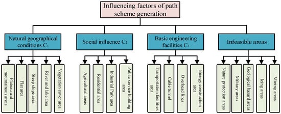
Figure 1. Geographical information constraint evaluation system.

2.1.2. Spatial Weight Quantification of Geographical Environmental Factors

In distribution network line planning, geographical environmental constraints exhibit multi-dimensional and multi-scale complexity, creating an urgent need for a systematic method to convert qualitative constraints into quantitative weights. To address this, IAHP is introduced, which is an extension of the traditional Analytic Hierarchy Process (AHP). By replacing fixed scale values with interval numbers, IAHP can more accurately characterize experts’ ambiguous judgments regarding the importance of factors [20]. Through interval operations and possibility degree ranking, IAHP generates weight intervals that integrate both subjective experience and objective data, ultimately converging to a definite value. The process is shown in Figure 2.

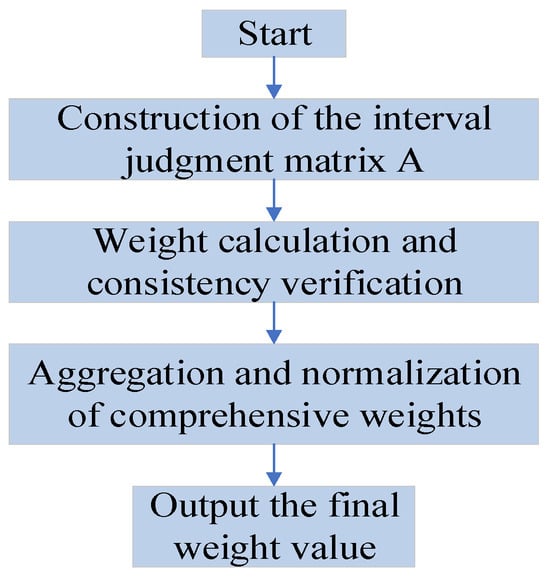
Figure 2. Flow chart of IAHP.

Step 1: Construction of the interval judgment matrix $A$. After determining the structural relationships of the criterion layer and the internal connections of the factor layer based on the geographical information hierarchical model in Figure 1, a pairwise comparison of the importance of factors is conducted. The 1–9 scale method is employed to establish and generate the interval number judgment matrix. Suppose a certain hierarchy contains a factor set; the interval number matrix is then defined as

$$A_{ij}={([a_{ij}^{-},a_{ij}^{+}])}_{n\times n}$$

(1)

where $a_{ij}^{-}$ and $a_{ij}^{+}$ represent the lower and upper limits of the importance of factor $u_i$ relative to factor $u_j$, respectively, they satisfy the reciprocal property that $a_{ji}^{-}=1/a_{ij}^{+}$ and $a_{ji}^{+}=1/a_{ij}^{-}$, and the diagonal elements satisfy $a_{ii}^{-}=a_{ii}^{+}=1$.

Step 2: Weight calculation and consistency verification. After checking the consistency with the method in reference [21], decompose the interval judgment matrix $A$ into deterministic matrices $A^{-}={(a_{ij}^{-})}_{n\times n}$ and $A^{+}={(a_{ij}^{+})}_{n\times n}$, calculate the eigenvectors ${\omega }^{-}$ and ${\omega }^{+}$, respectively, and obtain the interval weight vector:

$$W=[\sqrt{{\displaystyle \sum _{j=1}^n\frac{1}{{\displaystyle \sum _{i=1}^n{a}_{ij}^{+}}}}}{\omega }^{-},\sqrt{{\displaystyle \sum _{j=1}^n\frac{1}{{\displaystyle \sum _{i=1}^n{a}_{ij}^{-}}}}}{\omega }^{+}]$$

(2)

The weight vector between the factor layer and the criterion layer is denoted as $W_G$, and the weight vector between the criterion layer and the goal is $W_R$. The weight between the factor layer and the goal is obtained as

$$W_z=W_G\times W_R$$

(3)

To convert the weight values from interval numbers to point values via the possibility degree formula, let the i and j elements in the weight $W_z$ be $W_{z,i}=[W_{\mathrm{z},i}^{-},W_{\mathrm{z},i}^{+}]$ and $W_{z,j}=[W_{z,j}^{-},W_{z,j}^{+}]$, respectively. Then

$$P(W_{z,i}\ge W_{z,j})={\displaystyle \frac{\max (0,L(W_{z,i})+L(W_{z,j})-\max (0,W_{z,j}^{+}-W_{\mathrm{z},i}^{-}))}{L(W_{z,i})+L(W_{z,j})}}$$

(4)

where $L(W_1)={{\omega }_1}^{+}-{{\omega }_1}^{-}$ and $L(W_2)={\omega }_2^{+}-{\omega }_2^{-}$ denote the interval lengths.

Step 3: Aggregation and normalization of comprehensive weights. By comparing the elements in the weight $W_z$ and establishing a possibility degree judgment matrix $P={[p_{ij}]}_{n\times n}$, where $p_{ij}=P(W_{z,i}>W_{z,j})$, the final comprehensive weight vector is calculated by the following formula:

$$x_i={\displaystyle \frac{{\displaystyle \sum _{j=1}^n{P}_{ij}+n/2-1}}{n(n-1)}},(i=1,2,\dots ,n)$$

(5)

2.2. Grid Modeling of Spatial Load Distribution

In the practice of distribution network grid-based planning, discrete distribution transformer area load points pose practical challenges to planning work. These load points not only exhibit scattered and uneven spatial distribution that fails to reflect the overall agglomeration trend but also lead to deviations in capacity assessment due to differences in temporal load characteristics across various regions. More critically, the discrete distribution form lacks spatial continuity, making it difficult to integrate geographical environmental constraints with load data for unified modeling.

To address these issues, it is particularly necessary to process discrete load points through spatial aggregation and continuous expression methods. This processing approach can construct a grid model of spatial load distribution suitable for grid-based planning while preserving the spatial distribution patterns and complementary characteristics of the load. Furthermore, it provides accurate data support for subsequent path optimization and capacity configuration tasks. Based on the different operational characteristics of load points x and y, the load complementarity coefficient can be derived as follows:

$$c_{ij}=1-{\displaystyle \frac{v_{ij}}{v_{\mathrm{avg},ij}}}$$

(6)

where $v_{ij}$ denotes the fluctuation rate after the combination of load points $i$ and $j$, and $v_{\mathrm{avg},ij}$ denotes the reference fluctuation rate of load point $i$ and $j$.

$$v_{ij}={\displaystyle \frac{{\sigma }_{ij}}{{\mu }_{ij}}}$$

(7)

$$v_{\mathrm{avg},ij}={\displaystyle \frac{{\sigma }_i+{\sigma }_j}{{\mu }_i+{\mu }_j}}$$

(8)

where ${\mu }_i$ and ${\mu }_j$ are the mean values of load points $f_i(t)$ and $f_j(t)$, respectively; ${\sigma }_i$ and ${\sigma }_j$ are the variances of load points $f_i(t)$ and $f_j(t)$, respectively; ${\mu }_{ij}$ and ${\sigma }_{ij}$ are the mean value and variance of the combined load point $f_{ij}(t)$.

Considering the non-uniform spatial distribution characteristics of distribution network load points, the density peak clustering algorithm is adopted for clustering analysis of load points [22]. This algorithm identifies high-density regions as cluster centers by calculating the local density ${\rho }_i$ and the relative distance ${\delta }_i$:

$${\rho }_i={\displaystyle \sum _{j\ne i}\chi (d_{ij}-d_c)}\cdot (1+\alpha \cdot c_{ij})$$

(9)

$${\delta }_i=\underset{j:{\rho }_j>{\rho }_i}{\min }{d}_{ij}$$

(10)

where $d_{ij}$ is the Euclidean distance between load points $i$ and $j$; $d_c$ is the cutoff distance, taken as 500 m; $\chi (·)$ is an indicator function, where $\chi (·)=1$ if $(·)<0$, otherwise $\chi (·)=0$; α is a regulation coefficient. Points with both high local density and high relative distance are selected as cluster centers, and the remaining load points are assigned to the corresponding clusters based on the nearest neighbor principle, forming $K$ load clusters ${\mathsf{\Omega }}_1,{\mathsf{\Omega }}_2\dots ,{\mathsf{\Omega }}_K$. Then, the kernel function bandwidth is

$$h_k={\displaystyle \frac{1}{2}}\cdot \beta \cdot \underset{i,j\in {\mathsf{\Omega }}_k}{\max }{d}_{ij}$$

(11)

where $\beta$ is a regulation coefficient that controls the interpolation range, taken as 1.5. According to the condition of load clusters, the cluster average complementarity coefficient ${\overline{c}}_k$, the local complementarity coefficient of load points ${\overline{c}}_i$, and the complementarity coefficient weight ${\alpha }_k$ can be obtained:

$${\overline{c}}_k={\displaystyle \frac{2}{m_k\left(m_k-1\right)}}{\displaystyle \sum _{\begin{array}{c}i<j\\ i,j\in {\mathsf{\Omega }}_k\end{array}}{c}_{ij}}$$

(12)

$${\overline{c}}_i={\displaystyle \frac{1}{m_k-1}}{\displaystyle \sum _{\begin{array}{c}j\ne i\\ j\in {\mathsf{\Omega }}_k\end{array}}{c}_{ij}}$$

(13)

$${\alpha }_k=\min \left(\gamma ,{\overline{c}}_k\right)$$

(14)

where $m_k$ is the number of load points within the cluster; $\gamma$ is a regulation coefficient that limits the correction intensity to avoid excessive amplification. After dividing the load clusters, the spatially continuous load density distribution can be further calculated as

$${\lambda }_k(x,y)={\displaystyle \frac{1}{m_k}}{\displaystyle \sum _{i\in {\mathsf{\Omega }}_k}{\mu }_i}\left(1+{\alpha }_k{\overline{c}}_i\right)K_k\left({\displaystyle \frac{d((x,y),(x_i,y_i))}{h_k}}\right)$$

(15)

where $K(·)$ is a kernel function, and the Epanechnikov kernel function is selected; $d$ denotes the geographical distance. By combining with the GIS platform to partition the geographical space into multiple grid cells with equal size, the load density value assigned to each grid cell is

$$\lambda (m,n)={\displaystyle \frac{1}{9}}{\displaystyle \sum _{p=-1}^1{\displaystyle \sum _{q=-1}^1{\lambda }_k}}\left(m\cdot s+{\displaystyle \frac{2s+p\cdot s}{4}},n\cdot s+{\displaystyle \frac{2s+q\cdot s}{4}}\right)$$

(16)

$${\lambda }^{\prime }={\displaystyle \frac{\lambda (m,n)-{\lambda }_{\min }(m,n)}{{\lambda }_{\max }(m,n)-{\lambda }_{\min }(m,n)}}$$

(17)

where $\lambda (m,n)$ is the load density value of the grid cell; $s$ denotes the grid resolution; ${\lambda }^{\prime }$ represents the load density weight. Through the aforementioned “partitioning-interpolation-aggregation” method, a grid map of spatial load distribution is constructed.

3. Distribution Network Line Optimization Method

3.1. Grid Definition of Lines Based on Bresenham Algorithm

To quantify the impacts of distribution network lines traversing different geographical constraints and load densities, it is necessary to divide the lines into N continuous sub-segments with variable lengths. The Bresenham algorithm is employed to discretize the sub-segments into grid mappings, so as to determine the grid conditions traversed by the path, thereby accurately calculating the equivalent geographical cost and load benefit of the entire line:

$$D_2={\displaystyle \sum _{i=1}^N{d}_i\times \frac{{\displaystyle \sum _{e=1}^{N_g}{x}_e}}{N_g}}-\eta \cdot {\displaystyle \sum _{i=1}^N{d}_i\times \frac{{\displaystyle \sum _{e=1}^{N_g}{\lambda }_e^{\prime }}}{N_g}}$$

(18)

where $d_i$ is the length of a certain sub-segment; $N_g$ is the total number of grids traversed by this sub-segment; $x_e$ denotes the weight of geographical environmental factors for grid e; $\eta$ is the load benefit adjustment coefficient, taken as 0.3, which quantifies the benefit gain brought by the line traversing high-load-density regions; ${\lambda }_e^{\prime }$ represents the load density weight of grid e.

The core idea of the Bresenham algorithm is to determine the grid cells traversed by a straight-line path via an error accumulation mechanism [23]. Given a start point $(x_1,y_1)$ and an end point $(x_2,y_2)$ in the grid map and connecting them into a line segment, the line segment is first transformed into a gentle line segment as shown in Figure 3 through operations such as translation and flipping. According to whether the absolute value of the line segment slope is greater than 1, the coordinate system is rotated until the main increasing direction is the x-axis or y-axis. With a step size of 0.5 grid in the main direction as the progressive step, intermediate detection points are generated along the path direction. When moving grid by grid along the main direction, the error term $\epsilon$ is dynamically updated. For a line segment with a slope of $m=\Delta y/\Delta x$, the error update rule is

$${\epsilon }_{\mathrm{new}}={\epsilon }_{\mathrm{old}}+2\Delta y-\Delta x\cdot \mathrm{sign}(\Delta x)$$

(19)

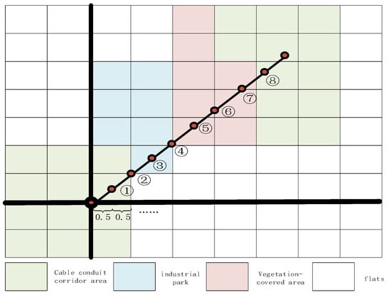
Figure 3. Pixelated detection of line grid based on Bresenham algorithm.

If $\epsilon \ge 0$, the coordinate in the secondary direction is incremented, and ${\epsilon }_{\mathrm{new}}={\epsilon }_{\mathrm{old}}-2\Delta x$ is reset. This process generates the coordinate sequence penetrated by the path grid by grid, forming a discretized path representation.

3.2. Improved A-Star Algorithm

As a classic heuristic graph search algorithm, the A-star algorithm is one of the most effective direct search methods for solving the shortest path in static road networks [24]. By incorporating a heuristic evaluation function, the heuristic A-star algorithm comprehensively evaluates the cost value of each search node, selects nodes by comparing the cost values of nodes to be expanded, and establishes a state space during the search process, thereby guiding the search process to converge toward the optimal solution [25].

During the operation of the heuristic A-star algorithm, the search state space is established by constructing a set of nodes to be explored (OPEN list) and a set of expanded nodes (CLOSE list). The OPEN list stores nodes to be processed that carry information on the estimated comprehensive cost; the CLOSE list records nodes that have completed topological analysis to prevent invalid backtracking. In each step of node search, the candidate node with the minimum comprehensive cost is extracted from the OPEN list, added to the CLOSE list for expansion, and the costs of the new and old paths are compared to dynamically update the OPEN list and CLOSE list. This ensures that the storage structure always reflects the optimal topological information. The A-star algorithm defines the node evaluation function as

$$f(n)=g(n)+h(n)$$

(20)

where $g(n)$ represents the actual accumulated cost from the start node $S_0$ to the current node $S_n$, including quantifiable parameters such as line length, geographical weight, and load density; $h(n)$ is a heuristic function term that estimates the remaining cost from the current node $S_n$ to the target node $S_N$; $f(n)$ is the comprehensive evaluation of node value, which determines its ranking in the search priority queue. The calculation process of the A-star algorithm is shown in Figure 4 and Algorithm 1. Each node state evaluates the value of every other search position, and the parent node records the optimal node obtained during the search process, which is used to backtrack the optimal path. The search process from the start point to the end point is as follows.

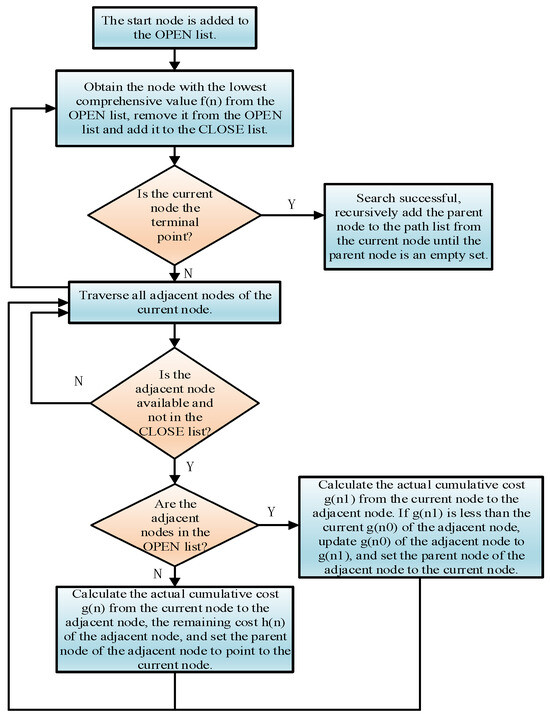
Figure 4. Flowchart of A-star algorithm.

Step 1: Add the start point to the OPEN list, initialize its cost $g(S_0)$, and set $f(S_0)=h(S_0)$.

Step 2: Extract the node n with the smallest $f(n)$ from the OPEN list; if n is the end point N, backtrack the path and terminate; otherwise, add n to the CLOSE list and generate its subsequent feasible node set.

Step 3: For each subsequent node m adjacent to n, if it is in an infeasible region or in the CLOSE list, traverse again; otherwise, calculate the new comprehensive cost $f(m)$ for each feasible node. If the adjacent node is not in the OPEN list, record it as the parent node and update the cost; if the adjacent node is in the OPEN list but the new cost is lower, record the parent node and update its $g(m)$ and $f(m)$.

Repeat Steps 2–3 until the end point is added to the OPEN list. Backtrack from the end point and form a route along the grid corresponding to each parent node until the start point, obtaining the optimal line.

Algorithm 1. Improved A-Star Path Planning.

Input: Grid matrix G, load density map L, start S, goal T Strategy mode M, parameters (η, A1) Output: Optimal path P   1:    C ← ComputeCostMap(G, L, M, η, A1)     //Equation (18) 2:    Initialize priority queue Q, closed set Cₗ 3:    Initialize g(S) = 0, f(S) = h(S, T) 4:    Q.push(S, f(S)) 5: 6:    while Q not empty do 7:            n ← Q.pop() 8:            if n = T then 9:                    return ReconstructPath(P) 10:          Cₗ.add(n) 11: 12:           for each neighbor m of n do 13:                  if m ∉ G or m ∈ Cₗ or C(m) = ∞ then 14:                           continue 15: 16:                  gₜₑₘₚ ← g(n) + ‖n-m‖·C(m)          //Actual cost 17: 18:                  if m ∉ Q or gₜₑₘₚ < g(m) then 19:                          g(m) ← gₜₑₘₚ 20:                          f(m) ← g(m) + h(m, T)          //Equation (20) 21:                          parent(m) ← n 22:                          Q.update(m, f(m)) 23: 24:    return ∅ //No feasible path

3.3. Line Smoothing and Engineering Feasibility Constraints

The optimal line derived from the improved A-star algorithm exhibits zigzag characteristics with sharp turns, resulting in uneven spacing between pylons, concentrated mechanical stress, and also inducing distortion in cost evaluation. Thus, a path smoothing optimization method based on Bezier curves should be employed. By integrating parametric curve modeling with geographical constraints, the collaborative optimization of path smoothness and geographical adaptability is realized. Bezier curves define a continuous and smooth curve via the convex combination of control points, with concise mathematical expressions and global controllability, making them suitable for path smoothing problems. For a planned line consisting of a node sequence $\{p_0,p_1,\dots ,p_n\}$, an n-th order Bezier curve is defined [26], and its parametric equation is

$$C(t)={\displaystyle \sum _{i=1}^n{B}_{i,n}(t)p_i,t\in [0,1]}$$

(21)

where $B_{i,n}(t)=(\begin{array}{c}n\\ i\end{array})t^i{(1-t)}^{n-1}$ is the Bernstein basis function. In the path smoothing for distribution networks, a cubic Bezier curve (n = 3) is generally sufficient, and its expression is

$$C(t)={(1-t)}^3{p}_0+3t{(1-t)}^2{p}_1+3t^2(1-t)p_2+t_3{p}_3$$

(22)

This curve satisfies $C(0)=p(0),C(1)=p_3$, and its first-order derivative is continuous, which can ensure a smooth transition of the route curvature. Calculate the curvature extreme points for the original path generated by A-star and generate control points:

$$k_i={\displaystyle \frac{‖(x_{i+1}-x_i)(y_{i-1}-y_i)-(x_{i-1}-x_i)(y_{i+1}-y_i)‖}{{({(x_{i+1}-x_i)}^2+{(y_{i+1}-y_i)}^2)}^{3/2}}}$$

(23)

where points satisfying $k_i>k_{th}$ are selected as the initial candidate set of control points $Q_{\mathrm{raw}}$. Down sampling is performed on $Q_{\mathrm{raw}}$ to retain points with significant geometric features, forming the final control point sequence $\{Q_0,Q_1,\dots ,Q_k\}$. Moreover, $Q_0=p_1$ and $Q_k=p_n$ are forcibly set to ensure that the start and end points of the smoothed path are consistent with those of the original path. The average curvature $\overline{k}$ and corner energy $E$ are used to quantify the overall smoothness of the path:

$$\overline{k}={\displaystyle \frac{1}{n-2}}{\displaystyle \sum _i^{n-2}{k}_i}$$

(24)

$$E={\displaystyle \sum _{i=1}^{n-2}{\left[\arccos \left(\frac{(x_i-x_{i-1})(x_{i+1}-x_i)+(y_i-y_{i-1})(y_{i+1}-y_i)}{\sqrt{{(x_i-x_{i-1})}^2+{(y_i-y_{i-1})}^2}\cdot \sqrt{{(x_{i+1}-x_i)}^2+{(y_{i+1}-y_i)}^2}}\right)\right]}^2}$$

(25)

Incorporate curvature constraints and obstacle avoidance constraints to ensure the generated curve conforms to practical planning requirements and avoids infeasible areas:

$$\tau (t)={\displaystyle \frac{‖B^{\prime }(t)\times B^{″}(t)‖}{{‖B^{\prime }(t)‖}^3}}\le {\displaystyle \frac{1}{R_{\min }}}$$

(26)

$$\Delta C_{i,k}={\displaystyle \sum _{j}k\cdot \frac{\max (d_j-r_{\mathrm{safe}},0)}{d_j}}\cdot (C-O_j)$$

(27)

where $R_{\min }$ denotes the minimum allowable bending radius of the cable; $\tau (t)$ represents the line curvature. $\Delta C_{i,k}$ signifies the deviation for adjusting the center position when the curve contacts an infeasible region; $d_j$ is the distance from the control point to the obstacle surface; $C$ is the center coordinate; $O_j$ is the nearest point on the surface of the j-th obstacle; k is the elastic coefficient; $r_{\mathrm{safe}}$ is the safe distance. Meanwhile, the arc radius is reduced to $R^{(t+1)}=0.95\cdot R^{(t)}$.

After path smoothing, the comprehensive cost of each line is calculated as follows:

$$D{=\mathrm{A}}_l\cdot l_i+D_1$$

(28)

where ${\mathrm{A}}_l$ denotes the unit–length construction cost of the line; $l_i$ represents the total length of the smoothed line; $D_1$ is the equivalent geographical cost and load benefit of the line.

4. Case Study

4.1. Case Description

The case adopted in this chapter is derived from the high-definition map system of a feeder in a specific area of Guangdong Province; the map depicts the 10 kV single-radial overhead line structure in this region, where the voltage class of the upstream substation is 110 kV, the total length of the line is 12.06 km, the power supply radius is 7.28 km, and the line model is LGJ-70 mm². The planned area encompasses various types of geographical environments, including municipal roads, agricultural farmland, ecological protection zones, residential buildings, and artificial fish ponds, and this feeder is primarily responsible for supplying electricity for residential daily use and agricultural farmland operations. Specific details are illustrated in Figure 5, which shows the locations of load distribution areas, the 110 kV substation, and tie switches; a number of users connect to adjacent distribution areas for power supply according to their geographical locations, these distribution areas are mainly distributed along streets adjacent to residential buildings, and the path distribution is complex, with statistics showing there are 68 streets and 152 roads in total. With respect to load information, there are 23 transformers in operation, among which 14 are public transformers with a total connected load of approximately 0.4 MW, and 9 are dedicated transformers with a total connected load of approximately 0.12 MW.

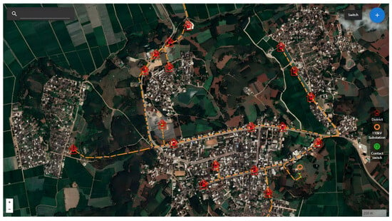
Figure 5. GIS diagram of 10 kV distribution network.

Based on the GIS conditions of this area, the quantitative grading strategy for geographical factors proposed in Section 2.1 was adopted to grade the geographical conditions present in the map, and the influence weights of geographical information factors on line construction costs were calculated. All geographical types within infeasible areas were set as obstacle grids, i.e., line construction must avoid these environments. The judgment matrix is constructed for the natural geographical conditions, infrastructure, and social impact criteria layer, as shown in Table 1. According to Equation (2), the weight vector of the criterion layer relative to the target layer is obtained as

$$W_G={[(0.7292,0.7455)(0.1792,0.1832)(0.0756,0.0876)]}^{\mathrm{T}}$$

Table 1. Judgment matrix of the criterion layer.

$\mathbf{A}$	$C_1$	$C_2$	$C_3$
$C_1$	(1, 1)	(4, 6)	(6, 8)
$C_2$	(1/6, 1/4)	(1, 1)	(2, 3)
$C_3$	(1/8, 1/6)	(1/3, 1/2)	(1, 1)

In the same way, the judgment matrix is constructed and the interval weight vector of each factor of the third layer to its corresponding criterion layer is calculated.

For the criterion layer of “natural geographical conditions”, the corresponding factors of the third layer are plateau and mountainous area, flat land, steep slope, river and lake area, and vegetation coverage area. The corresponding interval weight vector is recorded as $W_1$, and the calculation result is

$$W_1={[(0.1324, 0.1987)(0.0539,0.0985)(0.1583, 0.2171)(0.3521,0.4473)(0.2478,0.3456)]}^{\mathrm{T}}$$

For the criterion layer of “social impact”, the corresponding third layer factors are agricultural areas, residential areas, industrial parks, and public service buildings. The corresponding interval weight vector is recorded as $W_2$, and the determination result is

$$W_2={[(0.5012, 0.5517)(0.2018, 0.2513)(0.1985, 0.2482)(0.1957, 0.2451)]}^{\mathrm{T}}$$

For the criterion layer of “infrastructure”, the corresponding factors of the third layer are traffic facility area, cable pipe gallery, overhead lines and energy facilities, and the corresponding interval weight vector is recorded as $W_3$, and the calculation result is

$$W_3={[(0.3512, 0.4017)(0.1987, 0.2483)(0.2013, 0.2518)(0.3485, 0.3982)]}^{\mathrm{T}}$$

Following the same approach, the judgment matrix of the factor layer was constructed, and the comprehensive weight vector for all factors was derived based on Equations (3)–(5), with specific results presented in Table 2. It can be observed that some factors have similar weight values. To reduce the number of grid types in the subsequent grid map establishment and lower the computational cost of the path optimization algorithm, certain factors with similar influence degrees were merged into the same geographical type. Considering the merged factors and the actual geographical conditions present in the map, the geographical environment types established for the current case include the following:

Table 2. Comprehensive weights of various factors.

Factor	Weight Value	Factor	Weight Value
Mountainous area	0.105	Agricultural area	0.112
Plain area	0.062	Residential area	0.080
Lake area	0.153	Industrial park area	0.065
Vegetation area	0.141	Public service buildings	0.068
Steep slope	0.103	Transportation facility area	0.044
Overhead line	0.027	Cable corridor	0.025
Energy construction	0.041

① Cable Corridor Area: Cable corridors and overhead lines are merged, with the weight adopting that of the cable corridor factor; ② General Area: Flat land, industrial parks, and public service buildings are merged, with the weight adopting that of the flat land factor; ③ Infrastructure Area: Transportation facilities and energy construction areas are merged, with the weight adopting that of the transportation facility factor; ④ Residential and Farmland Areas: Their original factors are retained unchanged; ⑤ The coastal area where the distribution network is located is regarded as having no plateau mountains or steep slopes; ⑥ Vegetation and Lake Areas: Their original factors are retained unchanged; ⑦ No-Passing Area: As an infeasible area, its weight is set to infinity, and the planned line is strictly prohibited from passing through.

Combined with the comprehensive weight and load distribution of geographical environment factors, in order to balance the computational efficiency and sufficient spatial details to capture the key geographical and load distribution characteristics, 200 m was selected as the grid resolution, and the map was divided into multiple grid regions of equal size through the Tkinter toolkit of Python 3.11. Finally, a spatially gridded geographical map incorporating geographical constraints and load density was constructed. As shown in Figure 6, it can be observed that most areas of this region belong to farmland areas and vegetation-covered areas except for urban areas; there is an ecological protection zone in the center of the urban area, which also belongs to a highly vegetation-covered area; and the street grids in areas with dense residential distribution are represented as cable corridor areas and general areas.

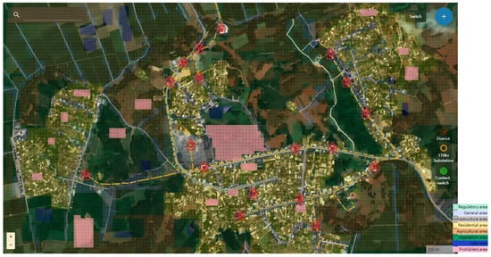
Figure 6. Distribution of geographic factors in grid based distribution network.

To verify the effectiveness of the distribution network line planning that incorporates geographical constraints and load density proposed in this study, it is necessary to merge several similar distribution area nodes in the figure. Figure 7 shows the situation after node merging and the modifications made to this power grid, which serves as the subsequent case, and presents the pre-planned lines between nodes based on actual geographical conditions. In the figure, red lines represent existing line connections, Node 0 is regarded as the power supply node, and black dashed lines are pre-planned lines whose connections need to cross different paths according to actual geographical conditions; Nodes 13–16 are potential new nodes to be added to this distribution network in the future.

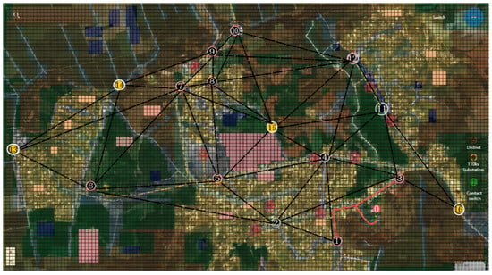
Figure 7. Modified pre-planning scenario of distribution network.

4.2. Result Analysis

4.2.1. Line Smoothing Analysis

Taking the lines between Nodes 3–4 and 5–14 as research examples, after performing grayscale processing on the background image, the obtained line schemes are shown in Figure 8 and Figure 9. In the figures, the red lines represent the initial line schemes obtained by direct solution using the A-star algorithm, while the green lines denote the optimized lines after smoothing processing.

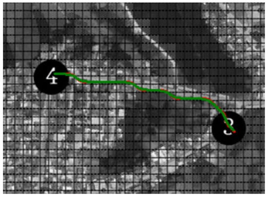
Figure 8. Line planning scheme for Nodes 3–4.

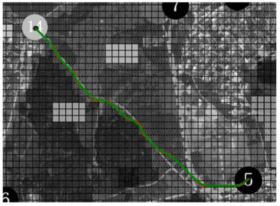
Figure 9. Line planning scheme for Nodes 5–14.

It can be seen from the quantitative analysis results in Table 3 that after path smoothing, the maximum curvature, average curvature, and corner energy of the path have all achieved significant reductions; the smoothed lines have effectively corrected the steep inflection points in the initial path, further improving the electrical safety and stability during the line construction process. Meanwhile, the smoothed lines can extend around the obstacle grid closest to the two nodes with optimal smoothness, which fully demonstrates that the method proposed in this study possesses excellent robustness and practical value.

Table 3. Comparison of lines between Nodes 3–4 and nodes 5–15 before and after smoothing.

Line	Maximum Curvature (rad/s)	Average Curvature (rad/s)	Corner Energy (rad2)
3–4 Before Smoothing	0.00297	0.00116	5.55
3–4 After Smoothing	0.00245	0.00103	2.58
5–14 Before Smoothing	0.00297	0.00116	8.64
5–14 After Smoothing	0.00241	0.00092	3.79

4.2.2. Analysis of Planning Schemes

To quantify the impact of planning logic on distribution network line construction, three schemes are set up in this case, all adopting chain connection. This method eliminates the interference caused by differences in connection modes through the series connection of nodes, ensuring that the comparison focuses on the core planning elements. Scheme 1: Distribution network line planning is conducted without considering geographical constraints, only taking load distribution into account. Scheme 2: Distribution network line planning is conducted without considering load distribution, only taking geographical constraints into account. Scheme 3: Based on the approach proposed in this study, distribution network line planning is conducted with simultaneous consideration of geographical constraints and load distribution. The distribution network line conditions after planning for each scheme are shown in the Figure 10, Figure 11 and Figure 12 below.

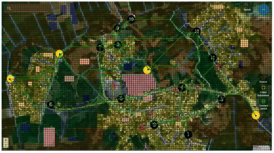
Figure 10. Expanded line results of each Node for Scheme 1.

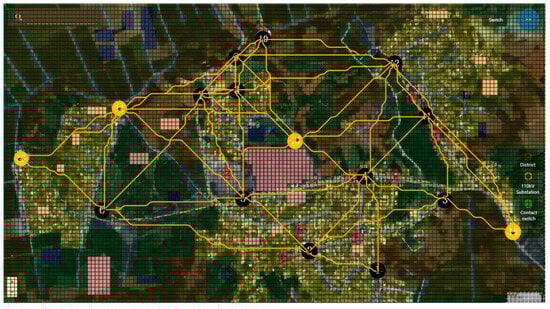
Figure 11. Expanded line results of each Node for Scheme 2.

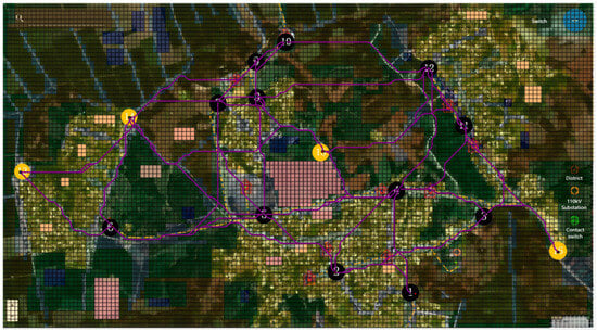
Figure 12. Expanded line results of each Node for Scheme 3.

The distribution network line planning results under different schemes are presented in Table 4. It can be concluded from the results that Scheme 1, due to the neglect of geographical constraints, achieves a relatively acceptable load benefit but incurs the highest total comprehensive cost among all schemes, which is attributed to the sharp surge in geographical cost. Scheme 2 ignores load distribution, which not only reduces the load benefit but also further impairs the overall economy owing to the redundant growth of basic cost. In contrast, Scheme 3 innovatively considers both geographical constraints and load distribution simultaneously. It not only avoids the drawback of excessively high geographical cost in Scheme 1 but also makes up for the deficiency of insufficient load benefit in Scheme 2, ultimately realizing the minimization of total comprehensive cost. This innovative planning idea with multi-constraint coordination not only demonstrates the economic advantages of planning but also provides a more efficient and breakthrough engineering reference for distribution network line construction, and it possesses distinct demonstration and reference value for similar planning tasks.

Table 4. Distribution network line planning results under different schemes.

Scheme	Total Comprehensive Cost (10,000 CNY)	Total Basic Cost (10,000 CNY)	Total Geographical Cost (10,000 CNY)	Total Load Benefit (10,000 CNY)
Scheme 1	4460.07	2751.76	1973.32	265.02
Scheme 2	3773.85	2975.93	962.78	164.86
Scheme 3	3767.14	2969.79	980.47	183.12

4.2.3. Comparison of Optimization Algorithms

To verify the superiority of the line planning algorithm proposed in this study, the Dijkstra algorithm [27] commonly used in engineering and the improved A-star algorithm proposed in this study are compared. Taking the lines between Nodes 7–13 and Nodes 8–14 as examples, the number of each grid type passed through and the total cost of the two methods are analyzed, as shown in Figure 13.

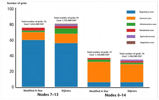
Figure 13. Grid conditions of planned lines under different algorithms.

It can be found from the results that the method in this paper outperforms the Dijkstra algorithm in both cost and performance of grid type traversal. The improved A-star algorithm sets increased weights for geographical and load factors in the heuristic function, which can guide the line to avoid high-cost geographical areas as much as possible and approach high load density areas, thereby reducing the overall construction cost. The lines obtained by both algorithms show little difference in the number of grids traversed. In the planning of Line 8–14, the greedy strategy of the Dijkstra algorithm leads to choosing a grid direction with a shorter distance in the early stage while ignoring geographical costs and load benefits, resulting in a higher total comprehensive cost. The method in this paper fully considers various existing geographical constraints and load distribution conditions in the planning process and is more in line with the practical application requirements in distribution network line planning.

5. Conclusions

This study proposes a distribution network line planning method integrating geographical information and load distribution. By establishing an IAHP-based geographical constraint hierarchical system, a peak load density clustering model, and an improved A-star algorithm, the coordinated optimization of geographical constraints and load density is achieved. This method effectively addresses the problem of separation between geographical constraints and load distribution in traditional planning, and significantly improves the economy and engineering feasibility of routes. The case study results show that the proposed method is comprehensively superior to conventional planning strategies, verifying that it has higher practicality and superiority in distribution network line planning and can provide reliable decision support for practical engineering.

Although the proposed method outperforms traditional approaches, it has certain limitations: First, the weights of geographical constraints are determined based on expert judgments via IAHP, which may introduce subjectivity. Second, the load density model assumes static loads and fails to consider temporal variations in the load. Third, the case study is only conducted for a specific region in Guangdong Province, and the method’s performance under other geographical and climatic conditions requires further validation. Additionally, the computational complexity will increase significantly when applied to ultra-large-scale power grids. Future research will focus on the following directions: (1) Integrating dynamic load forecasting to address temporal load variations; (2) Incorporating real-time environmental and meteorological data to enhance the method’s adaptability to dynamic scenarios; (3) Developing adaptive resolution strategies suitable for different network scales, so as to balance planning accuracy and computational efficiency; (4) Conducting validations across multiple geographical regions to improve the method’s universality in practical engineering applications.

References

- Cheng, L.; Yu, F.; Huang, P.; Liu, G.; Zhang, M.; Sun, R. Game-theoretic evolution in renewable energy systems: Advancing sustainable energy management and decision optimization in decentralized power markets. Renew. Sustain. Energy Rev. 2025, 217, 115776. [Google Scholar] [CrossRef]
- Nahman, J.M.; Peri, D.M. Radial distribution network planning under uncertainty by applying different reliability cost models. Int. J. Electr. Power 2020, 117, 105655. [Google Scholar] [CrossRef]
- Xiang, Y.; Zhou, L.; Su, Y.; Liu, J.; Huang, Y.; Liu, J.; Lei, X.; Sun, Z.; Xu, W.; Zhang, W. Coordinated DG-Tie planning in distribution networks based on temporal scenarios. Energy 2018, 159, 774–785. [Google Scholar] [CrossRef]
- Cheng, L.; Li, M.; Tan, C.; Huang, P.; Zhang, M.; Sun, R. Computational game-theoretic models for adaptive urban energy systems: A comprehensive review of algorithms, strategies, and engineering applications. Arch. Comput. Methods Eng. 2025. [Google Scholar] [CrossRef]
- Qin, Y.; Li, Z.; Ding, J.; Zhao, F.; Meng, M. Automatic optimization model of transmission line based on GIS and genetic algorithm. Array 2023, 17, 100266. [Google Scholar] [CrossRef]
- Tan, B.; Qiu, W.; Ding, Y.; Shi, H.; Yao, H.; Shen, X. Optimal planning method of renewable distributed generation for multiple prosumers participating in distribution networks. IOP Conf. Ser. Earth Environ. Sci. 2021, 675, 12137. [Google Scholar] [CrossRef]
- Fletcher, J.R.E.; Fernando, T.; Iu, H.H.; Reynolds, M.; Fani, S. Spatial Optimization for the Planning of Sparse Power Distribution Networks. IEEE T Power Syst. 2018, 33, 6686–6695. [Google Scholar] [CrossRef]
- Ebid, A.M.; Abdel-Kader, M.Y.; Mahdi, I.M.; Abdel-Rasheed, I. Ant Colony Optimization based algorithm to determine the optimum route for overhead power transmission lines. Ain Shams Eng. J. 2024, 15, 102344. [Google Scholar] [CrossRef]
- Nan, G.; Liu, Z.; Du, H.; Zhu, W.; Xu, S. Transmission Line-Planning Method Based on Adaptive Resolution Grid and Improved Dijkstra Algorithm. Sensors 2023, 23, 6214. [Google Scholar] [CrossRef]
- Yang, D.; He, T.; Du, B.; Wang, S.; Zhang, Z.; Zhang, S. Transmission line planning based on artificial intelligence in smart cities. Mob. Inf. Syst. 2022, 2022, 2010189. [Google Scholar] [CrossRef]
- Chen, J.; Yang, Y.; Peng, L.; Yang, L.; Han, Y.; Ge, X. Overhead line path planning based on deep reinforcement learning and geographical information system. Int. J. Electr. Power 2025, 165, 110468. [Google Scholar] [CrossRef]
- Pesántez, G.; Guamán, W.; Córdova, J.; Torres, M.; Benalcazar, P. Reinforcement Learning for Efficient Power Systems Planning: A Review of Operational and Expansion Strategies. Energies 2024, 17, 2167. [Google Scholar] [CrossRef]
- Sharma, K.K.; Seal, A. Outlier-robust multi-view clustering for uncertain data. Knowl.-Based Syst. 2021, 211, 106567. [Google Scholar] [CrossRef]
- Ni, Y.; Zeng, X.; Liu, Z.; Yu, K.; Xu, P.; Wang, Z.; Zhuo, C.; Huang, Y. Faulty feeder detection of single phase-to-ground fault for distribution networks based on improved K-means power angle clustering analysis. Int. J. Electr. Power 2022, 142, 108252. [Google Scholar] [CrossRef]
- Madadi, S.; Mohammadi-Ivatloo, B.; Tohidi, S. A Data Clustering Based Probabilistic Power Flow Method for AC/VSC-MTDC. IEEE Syst. J. 2019, 13, 4324–4334. [Google Scholar] [CrossRef]
- Sadeghian, O.; Oshnoei, A.; Kheradmandi, M.; Khezri, R.; Mohammadi-Ivatloo, B. A robust data clustering method for probabilistic load flow in wind integrated radial distribution networks. Int. J. Electr. Power 2020, 115, 105392. [Google Scholar] [CrossRef]
- Cheng, L.; Wei, X.; Li, M.; Tan, C.; Yin, M.; Shen, T.; Zou, T. Integrating Evolutionary Game-Theoretical Methods and Deep Reinforcement Learning for Adaptive Strategy Optimization in User-Side Electricity Markets: A Comprehensive Review. Mathematics 2024, 12, 3241. [Google Scholar] [CrossRef]
- Guo, S.; Gong, J.; Shen, H.; Yuan, L.; Wei, W.; Long, Y. DBVSB-P-RRT*: A path planning algorithm for mobile robot with high environmental adaptability and ultra-high speed planning. Expert Syst. Appl. 2025, 266, 126123. [Google Scholar] [CrossRef]
- Cheng, L.; Peng, P.; Huang, P.; Zhang, M.; Meng, X.; Lu, W. Leveraging evolutionary game theory for cleaner production: Strategic insights for sustainable energy markets, electric vehicles, and carbon trading. J. Clean. Prod. 2025, 512, 145682. [Google Scholar] [CrossRef]
- De-shun, L.; Kai-li, X. Research on the subjective weight of the risk assessment in the coal mine system based on GSPA-IAHP. Procedia Eng. 2011, 26, 1956–1963. [Google Scholar] [CrossRef]
- Moses, V.; Hatherley, R.; Tastan Bishop, Ö. Bioinformatic characterization of type-specific sequence and structural features in auxiliary activity family 9 proteins. Biotechnol. Biofuels 2016, 9, 239. [Google Scholar] [CrossRef] [PubMed]
- Hou, J.; Zhang, A.; Qi, N. Density peak clustering based on relative density relationship. Pattern Recogn. 2020, 108, 107554. [Google Scholar] [CrossRef]
- Stogiannopoulos, T.; Theodorakopoulos, I. Curved Text Line Rectification via Bresenham’s Algorithm and Generalized Additive Models. Signals 2024, 5, 705–720. [Google Scholar] [CrossRef]
- Zhang, Z.; Wu, J.; Dai, J.; He, C. A Novel Real-Time Penetration Path Planning Algorithm for Stealth UAV in 3D Complex Dynamic Environment. IEEE Access 2020, 8, 122757–122771. [Google Scholar] [CrossRef]
- Yang, T.; Zou, L.; Wu, Z.; Chen, W. An improved A-star algorithm coupled with graph division and AIS data for ship path planning. Ocean Eng. 2025, 330, 121234. [Google Scholar] [CrossRef]
- Bulut, V. Path planning of mobile robots in dynamic environment based on analytic geometry and cubic Bézier curve with three shape parameters. Expert Syst. Appl. 2023, 233, 120942. [Google Scholar] [CrossRef]
- Zhu, D.; Sun, J. A New Algorithm Based on Dijkstra for Vehicle Path Planning Considering Intersection Attribute. IEEE Access 2021, 9, 19761–19775. [Google Scholar] [CrossRef]
Disclaimer/Publisher’s Note: The statements, opinions and data contained in all publications are solely those of the individual author(s) and contributor(s) and not of MDPI and/or the editor(s). MDPI and/or the editor(s) disclaim responsibility for any injury to people or property resulting from any ideas, methods, instructions or products referred to in the content. |
© 2025 by the authors. Licensee MDPI, Basel, Switzerland. This article is an open access article distributed under the terms and conditions of the Creative Commons Attribution (CC BY) license.