Abstract
Traditional vehicle emergency braking research suffers from inaccurate maximum road adhesion coefficient identification and suboptimal wheel slip ratio control. To address these challenges in electronic hydraulic braking systems’ anti-lock braking technology, firstly, this paper proposes a CDOA-SENet-CNN neural network to precisely estimate the maximum road adhesion coefficient by monitoring and analyzing the braking process. Secondly, correlation curves between peak adhesion coefficients and ideal slip ratios are established using the Burckhardt model and CarSim 2020, and the estimated maximum adhesion coefficient from the CDOA-SENet-CNN network is used with these curves to determine the optimal slip ratio for the single-neuron integral sliding mode control (SNISMC) algorithm. Finally, an SNISMC control strategy is developed to adjust the wheel slip ratio to the optimal value, achieving stable wheel control across diverse road surfaces. Results indicate that the CDOA-SENet-CNN network rapidly and accurately estimates the peak braking surface adhesion coefficient. The SNISMC control strategy significantly enhances wheel slip ratio control, consequently increasing the effectiveness of vehicle brakes. This paper introduces an innovative, stable, and efficient solution for enhancing vehicle braking safety.
1. Introduction
Throughout the past several years, the automobile industry has seen vigorous innovation. Against this backdrop, vehicle driving safety has gained prominence as a key industry focus. Within the electronic hydraulic braking (EHB) system, the anti-lock braking system (ABS) plays a pivotal role. It stops wheels from locking during braking, preserving higher tire–ground adhesion. This helps to ensure that the vehicle remains secure and manageable.
Current investigations into braking systems are primarily divided into two key areas. The first area focuses on determining the peak road surface adhesion coefficient [1,2,3,4], which largely hinges on the frictional properties between the road and the tire. Usually, a tire model can be established based on this characteristic, and the maximum adhesion coefficient of the road surface can be estimated based on the tire model. Common tire models include the Burckhardt model [5], the Pacejka model [6], and the Kiencke model [7]. Among them, the Burckhardt model is more common and can precisely describe the adhesion characteristics at the tire–road contact area. The second part involves creating the brake system’s controller [8,9,10,11]. According to the tire model, when the tire–road adhesion coefficient peaks, the corresponding wheel slip ratio is the optimal one. Once the wheel slip ratio matches this optimal value, the vehicle can slow down effectively and stop in the shortest possible distance. So, during braking, designing a robust controller that keeps the wheel slip ratio around the ideal level is crucial.
In the road recognition process, the peak coefficient of road surface adhesion can be obtained via visual recognition methods, mathematical modeling methods, and similarity calculation methods. Visual recognition methods primarily depend on image features and analyze road surface features online to assess the optimal road surface adhesion coefficient. Yanan Shen and others [12] utilized the VGG-16 convolutional neural network to extract image features and analyze the ideal slip ratio on the road surface. The mathematical model approach primarily employs vehicle tire models to forecast the optimal slip ratio for the vehicle at the moment. Hsin Guan and others [13] designed an optimal slip ratio identification estimator based on the Kiencke model using an improved forgetting factor recursive least squares algorithm. Shi Luo and others [14] developed an extended state observer to monitor the real speed of the vehicle and determine the wheel slip ratio’s adhesion coefficient under standard road conditions. They computed the current wheel’s adhesion coefficient using the vehicle’s physical model, then identified the road condition with the closest match to this adhesion coefficient under typical circumstances, deeming it the current road condition. Zejia He and others [15] fitted a ground slip map through a large number of data on the optimal slip ratio and peak adhesion coefficient of typical roads, and estimated the optimal slip ratio value based on the ground slip map and the adhesion coefficient of the existing road surface. The similarity calculation method primarily depends on the likeness of the typical road surface and the road surface beneath the vehicle to obtain the maximum adhesion coefficient. Houzhong Zhang and others [16] proposed a method following the principles of fuzzy rules. According to the typical road conditions, a fuzzy rule table is constructed, and then the similarity under the current road surface is assessed, and, finally, the maximum adhesion coefficient of the road is estimated. However, the visual recognition method relies on the real-time image transmission of the camera and the accuracy of the camera, and there are problems of camera data loss and image distortion. The road surface recognition calculation of the mathematical model method is too complicated, and, to a certain extent, it consumes most of the computing resources. Although the similarity calculation method reduces the amount of calculation to a certain extent, it contains certain human experience and relies on typical road condition estimation, so the estimation accuracy is not high.
In wheel slip ratio control, the design of controllers is primarily categorized into those utilizing physical models and those not relying on physical models. Controllers that do not rely on physical models include PID, fuzzy PID, adaptive PID, and anti-disturbance control. Controllers that rely on physical models include sliding mode control (SMC), model predictive control, etc. Abhas Kanungo and others [17] combined fuzzy control with PID to effectively shorten the braking distance. The ABS controller designed by Shi Luo and others [14] based on anti-disturbance control has good adaptability and stability. Haiqing Zhou and others [18] validated integral sliding mode control for wheel slip ratio management via experiments and simulations. Zejia He and others [15] proposed a model predictive control-based slip ratio strategy for good braking stability and safety. However, PID and fuzzy PID, relying on tuned parameters and experience, respectively, show poor dynamic and anti-interference performance during braking. Anti-interference control offers strong immunity but weak dynamics. Traditional sliding mode control has good dynamics but poor adaptability to complex conditions. Model predictive control is model-dependent and computationally intensive.
To tackle the previously mentioned challenges, this paper describes a CDOA-SENet-CNN neural network for estimating the peak road adhesion coefficient and employs SNISMC control to facilitate the wheel slip ratio rapidly reaching the optimal slip ratio. In terms of implementing deep learning models, this paper uses the MATLAB R2024b, whose deep learning toolbox supports the construction, training, and optimization of neural networks and features built-in network layer design, automatic differentiation, and GPU acceleration capabilities. The key innovations and contributions are as follows: it uses a convolutional neural network with SENet for road adhesion coefficient estimation, then uses the optimal slip ratio curve to precisely ascertain the optimal slip ratio; it designs a single-neuron integral sliding mode control strategy with a forgetting factor to effectively control the wheel slip ratio during braking.
This paper is structured as follows: Section 2 develops the vehicle dynamics model, streamlines it, scrutinizes the tire model, and plots the optimal slip ratio curve; Section 3 constructs the CDOA-SENet-CNN neural network; Section 4 presents SNISMC control; Section 5 carries out simulation experiments; Section 7 encapsulates the entire paper.
2. System Scheme
2.1. Single-Wheel Braking Model
The most common vehicle model is the four-wheel model [19]. As the driver applies pressure to the brake pedal, the vehicle begins to decelerate. Due to inertia, the front of the vehicle sinks relative to the rear, leading to an increase in the vertical load on the front axle. The front axle requires a greater braking force than the rear axle. Ignoring air resistance and rolling resistance of the wheels, the force analysis of a car during straight-line braking is shown in Figure 1 below:
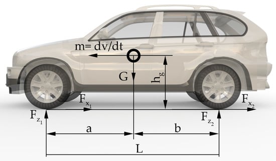
Figure 1.
Car force diagram.
From Figure 1, we can see that the moment equations of the vertical load of the front and rear wheels are as follows:
According to Equations (1) and (2), during braking, the front wheel is subjected to a greater braking force than the rear wheel, making it more likely to lock. Compared with the rear wheel slip ratio control, the front wheel slip ratio control requirements are more stringent. In summary, effective control of the front wheel implies that the rear wheel can also be controlled efficiently. To simplify the analysis, this paper focuses solely on front-wheel braking. The force analysis for the front wheel during braking is depicted in Figure 2.
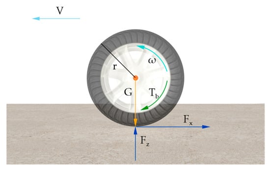
Figure 2.
Force diagram of single-wheel model.
In Figure 2, is the braking force applied to one wheel, is the longitudinal braking force of the ground acting on the wheel when the vehicle brakes, is the vertical force of the vehicle load transmitted to the ground via the tire, is the gravity of the vehicle, is the wheel speed, is the longitudinal speed of the vehicle when braking, and is the radius of the wheel.
From Figure 2, the vehicle dynamic model can be obtained as follows:
The physical model of wheel rotation is as follows:
During emergency braking scenarios, the wheel’s linear speed differs from the vehicle’s speed, leading the wheel to shift from rolling to a state of relative sliding. At this juncture, the slip between the wheel and ground depends on the wheel’s linear velocity and the vehicle’s speed. The specific equation is as follows:
where is the slip ratio.
2.2. Tire Model
The typical roads are the eight types of standard roads listed in the Burckhardt model [5], while the atypical roads are the roads that are not included in the types of standard roads listed in the Burckhardt model. This paper uses the typical road surface of the Burckhardt model and the CarSim 2020 simulated atypical road surface to explore the correlation between the adhesion coefficient of the tire–road contact and wheel slip ratio. As a semi-empirical model, the Burckhardt model can effectively capture the real-world physical interaction between tires and the ground. The model quantifies this interaction through three key parameters. The correlation between the tire–road adhesion coefficient is presented as follows:
where , , and are fitting coefficients. Differentiating Equation (6) yields the following:
Under the condition of , we can obtain the following:
From Equation (8), we can obtain the following:
Substituting Equation (9) into Equation (6), we obtain the following:
The typical road surface fitting coefficients and corresponding extreme points of the Burckhardt model are shown in Table 1. According to the extreme point data under each typical road condition in Table 1, the corresponding curve can be drawn, as shown in Figure 3.

Table 1.
Calibrating parameters for typical road surfaces.
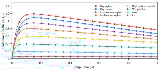
Figure 3.
Typical road surface curve.
Given that the Burckhardt model typically describes fewer road surfaces, and real road conditions are too complex for simple typical road surfaces to depict, it is essential to build the correlation between the tire adhesion coefficient and wheel slip ratio under atypical road circumstances. In the CarSim 2020 simulation software, thirteen atypical road models, including some of those with typical road surfaces from the Burckhardt model, are established to revise the Burckhardt model in realistic scenarios, with the curves of atypical road surfaces shown in Figure 4.
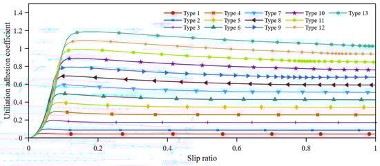
Figure 4.
Atypical road surface curve.
The maximum adhesion coefficients for the 13 simulated atypical roads are listed in Table 2.
Table 2.
Atypical pavement parameters.
2.3. Design of the Optimal Slip Ratio Curve
According to the optimal slip ratio and optimal adhesion coefficient under conventional road conditions determined by the Burckhardt model, combined with the atypical road surface data obtained based on the CarSim 2020 simulation software, an optimal slip ratio curve can be fitted through the curve of the extreme point. Through the optimal slip ratio curve, the estimated optimal adhesion coefficient is used to calculate the optimal slip ratio of the wheel under the present road. Because the Fourier function specifically captures the periodic law and has the advantages of flexibly fitting complex functions, this paper uses the Fourier function to fit the optimal slip ratio curve. The best slip ratio curve fitting equation can be obtained by fitting Fourier functions [20]:
In order to make the fitting curve more consistent with the actual scene, this paper uses the typical road of the Burckhardt model and the atypical road simulated by CarSim 2020 simulation software to fit, and the fitting parameters are shown in Table 3.
Table 3.
The fitting parameters of the optimal slip ratio curve.
The optimal slip ratio curves of the optimal adhesion coefficient and the optimal slip ratio for non-typical roads and typical roads are shown in Figure 5.
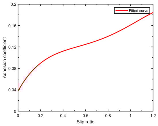
Figure 5.
Optimum slip ratio curve.
3. Design of Pavement Adhesion Coefficient Estimation System
3.1. Design of Convolutional Neural Networks Based on Squeeze-and-Excitation Networks
To leverage the optimal slip ratio curve for determining the optimal slip ratio, this section presents a convolutional neural network [21] incorporating SENet’s attention mechanism to assess the maximum road adhesion coefficient.
The Convolutional Neural Network (CNN) is mainly composed of convolutional layers, pooling layers, and fully connected layers. When using CNN to evaluate the road adhesion coefficient, the first step is to collect feature data such as vehicle speed, acceleration, slip ratio, and wheel rotation speed under various braking scenarios and different road conditions. The second step is data preprocessing: first, data cleaning operations remove missing, duplicate, and abnormal values, then filter out noise and irrelevant features, and, finally, normalize the data to unify the units. The third step is to extract effective information through convolution and pooling. Finally, the fully connected layer outputs the estimated value of the road adhesion coefficient. The process is shown in Figure 6.
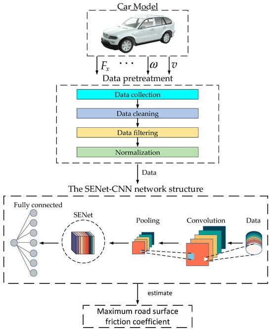
Figure 6.
Road adhesion coefficient prediction flow chart.
The convolutional layer applies convolutional operations to the input feature map using the convolution kernel and obtains the output feature map with a nonlinear activation function. The convolution operation calculation equation is as follows:
In Equation (10), is the jth output feature map obtained by the rth convolution operation; is the jth convolution kernel operated on the ith input feature map; is the jth convolution kernel bias of the rth layer network; is the nonlinear activation function.
Pooling layers lower computational demands by shrinking feature map sizes, which, in turn, reduces the dimensionality of data in higher layers. This process retains key features while minimizing redundant information. In view of the fact that hybrid pooling adaptively integrates the advantages of maximum/average pooling, taking into account both features and noise resistance, dynamic weight adjustment improves the robustness of the model, which is better than fixed single pooling. Therefore, this study adopts a hybrid pooling method, the formula of which is as follows:
where is a value that can randomly be either 0 or 1 in each pooling operation; is the output result of the kth feature map in the matrix region ; is the element situated at (p, q) in the rectangular region .
The feature maps extracted by the convolution layer and pooling layer are fully connected through a fully connected layer, and the size of the fully connected layer depends on the size of the output feature map of the previous layer (usually the pooling layer or convolution layer). The fully connected layer model can be represented as follows:
where is the fully connected layer input; is the weight matrix; is the bias vector.
During the process of vehicle braking, different data types have varying correlation degrees with the maximum road adhesion coefficient, and there are also certain relationships among these different data types. Therefore, when CNN mines data features, different feature channels have different importance. SENet [22] improves the performance of convolutional neural networks by introducing an attention mechanism of SENet in the channel dimension. SENet mainly consists of two parts: squeezing and excitation. Its structure can be as depicted in Figure 7 below.
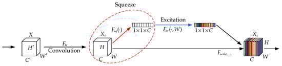
Figure 7.
SENet model.
Firstly, the squeezing operation mainly performs global average pooling on the input feature map to compress the channel dimension. The containing global information is mixed and pooled to obtain a feature vector of size . The calculation equation is as follows:
where and are the feature map sizes; is the input feature; C is the number of channels; is the local description operator generated by the squeezing operation.
Secondly, through two fully connected layers, the excitation operation calculates the importance weights of the channels. The first layer compresses the network dimension, and the second layer expands it back to its original size. The excitation equation is as follows:
In the equation, is the Relu function; is the activation function, here the Sigmoid function is used; is the attention weight.
Finally, each element of the original feature map is multiplied by the corresponding weight to produce the weighted feature map for each channel. The equation is as follows:
where is the output feature map.
3.2. Road Adhesion Coefficient Estimation Optimized Based on Chaos Dream Optimization Algorithm
With the aim of heightening the forecasting precision of the SENet-CNN neural network [23,24] for the maximum road adhesion coefficient, this paper incorporates the Chaos Dream Optimization Algorithm (CDOA) to refine the SENet-CNN neural network architecture’s parameters. The Dream Optimization Algorithm (DOA) [25] draws inspiration from the human dream mechanism and employs memory, forgetting, and replenishment strategies. On this basis, the chaos algorithm is integrated to optimize the population initialization phase of the DOA, leading to the development of the CDOA. CDOA possesses excellent global exploration and local convergence capabilities. Within CDOA, each individual corresponds to a set of CNN parameters, such as the count of convolutional layers, the quantity of convolutional kernels in each layer, and the dimensions of the convolutional kernel.
The flowchart of CDOA optimizing SENet-CNN neural network hyperparameters is shown in Figure 8.
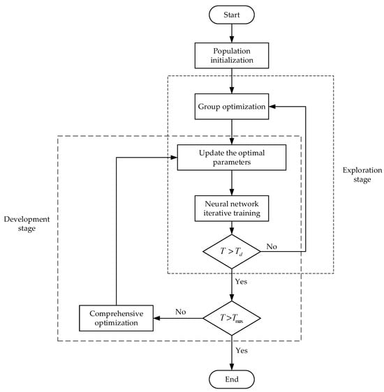
Figure 8.
CDOA optimization flowchart.
At the beginning, the population is initialized and categorized into clusters possessing varying memory capacities. During the iteration process of the exploration phase, the SENet-CNN neural network is iteratively trained based on the grouping. If the current iteration count reaches the maximum iteration count for the exploration phase, it then transitions from the exploration phase to the development phase. During the iteration process, in the development phase, the population no longer undergoes group optimization. Instead, based on the global optimal solution from the exploration phase, the SENet-CNN neural network is iteratively trained to search for local optimal solutions. When the maximum iteration count for the development phase is reached, the parameters corresponding to the system’s minimal fitness value are utilized as the training parameters for the SENet-CNN neural network. The CDOA has two phases: the exploration phase and the development phase.
According to the range of hyperparameters of the SENet-CNN neural network, the encoding population is initialized using Logistic mapping:
where is the nth encoding individual; is the branch parameter
After decoding the encoded individuals, the population is initialized as follows:
In the population, denotes the position of the ith individual.
During the exploration phase, the population is divided into five clusters with distinct memory abilities, and the optimal positions are identified through the forgetfulness supplementation strategy. This strategy integrates the global and local search capabilities, enabling individuals to forget and spontaneously adjust their position updates in the forgetfulness dimension. The equation for updating is as follows:
where indicates the location of the ith member in the jth coordinate at iteration t + 1; denotes the optimal location of the optimal individual in group q during iteration t in dimension j; and denote the minimum and maximum limits of the search in the jth dimension; is a randomly picked value that falls between 0 and 1; is the existing iteration number, is the maximum iteration number, and is the maximum iteration number in the exploration phase.
In the development phase, the iteration count progresses from to , the population is no longer grouped, and the forgetting and supplementing strategy is implemented. The update equation is as follows:
where denotes the ith individual’s position in the jth dimension at iteration t + 1; denotes the location of the optimal individual within the whole population at the jth dimension during the tth iteration.
Based on the principles of CDOA, when optimizing the SENet-CNN neural network using CDOA, the main evaluation indicators are the prediction deviation and total absolute error corresponding to each hyperparameter combination. After setting the CDOA parameters and iterating the training, the optimal hyperparameters of the SENet-CNN neural network are shown in Table 4.
Table 4.
Optimal hyperparameters of SENet-CNN.
4. Design of Brake Controller
4.1. Design of Integral Sliding Mode with Forgetting Factor
Using the CDOA-SENet-CNN algorithm, we estimate the peak road adhesion coefficient. Then, leveraging the optimal slip ratio curve for this coefficient, we calculate the ideal slip ratio for current road conditions. Finally, a suitable controller needs to be created to hold the wheel slip ratio adjacent to this optimal value.
Sliding mode control [26] has the characteristics of fast response and strong robustness. It achieves control by forcing the system to slide along a predetermined trajectory, but the traditional form is easily affected by integral saturation and historical errors. This paper proposes a new method for designing an integral sliding mode controller that incorporates a forgetting factor. By introducing the forgetting factor, the controller can effectively circumvent integral saturation and notably reduce historical error interference, ensuring control stability and speed, and enhancing overall control effectiveness.
By taking the derivative of Equation (5), the slip ratio change equation can be obtained as follows:
The slip ratio error is identified as follows:
Therefore, the integral synovial surface with forgetting factor is as follows:
In the equation, is the forgetting function, and its equation is as follows:
where is the memory stability coefficient. When is smaller, the integral error has less influence on the current control, and more attention is paid to the vehicle slip ratio error at the current moment; when is larger, the integral error has a greater influence on the current control, and it is believed that the error in the previous period has a certain degree of influence on the current vehicle operation.
By taking the derivative of Equation (24), the following result can be obtained:
Substituting Equation (23) into Equation (26) yields the following:
This introduces the exponential approach rate as follows:
Substituting obtained from Equation (4) into Equation (23), we obtain the following:
Substituting Equation (30) into Equation (28), we obtain the following:
From Equations (28) and (31), the formulation for the slip ratio controller is as follows:
where is the estimated optimal slip ratio.
So as to further analyze the stability of the controller, Lyapunov’s second method is applied to verification. Lyapunov’s second method is defined as: if a positive definite Lyapunov function is present and its derivative is either definitively or semi-definitively negative, the system is considered to be asymptotically stable.
Define the Lyapunov function as follows:
By differentiating Equation (29) as follows:
From the conditions of Equation (27), we can see that, since and are both positive numbers, the system exhibits asymptotic stability based on the Lyapunov criterion, and the system error converges to zero.
4.2. Design of Single Neuron Structure
In an integral sliding mode control with a forgetting factor, when the system approaches a stable state, the presence of the switching function in the convergence law still causes a certain degree of chattering in the system. To further reduce chattering, a single neuron is used to adjust the coefficient of the approach rate. The single-neuron integral sliding mode control (SNISMC) formed at this point is adaptive.
Figure 9 below illustrates the structure of an individual neuron.
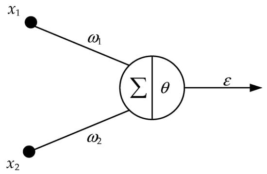
Figure 9.
Single neuron structure.
As shown in the figure above, and are the information received by the neuron, and are the connection strength or weight, and the linear weighted sum of the input information of a single neuron is obtained to obtain , which is expressed as follows:
Then the update equation of is as follows:
Based on the learning rule, the weight update formula is as follows:
where is the error criterion function; is the ith weight at time k; is the learning rate.
The definition is as follows:
When , increases and the state quickly approaches the sliding surface; when , decreases and the chattering is reduced. Similarly, when the system is , the state at the moment on the sliding surface quickly approaches the stable origin; when , the system overshoot is reduced and the chattering at the moment close to the steady state is weakened.
5. Simulation
5.1. Simulation Model and Parameter Settings
To verify the proposed strategy’s validity and efficacy in this experiment, a joint simulation was executed using MATLAB/Simulink R2024b and CarSim 2020 simulation software, establishing the vehicle motion and control systems. In CarSim 2020, a C-class vehicle served as the subject, with parameters detailed in Table 5, and the control system layout is illustrated in Figure 10. The experiment took place on a straight road with varying road adhesion coefficients. The control system includes an optimal slip ratio estimator, a vehicle model, and a single-neuron integral sliding-mode controller. The estimator comprises a CDOA-SENet-CNN neural network and a fitted optimal slip ratio curve. It calculates the current maximum road adhesion coefficient from vehicle braking characteristics and determines the optimal slip ratio via the curve. The SNISMC uses the estimator’s output as a reference to generate control signals for the vehicle model.
Table 5.
System parameters.
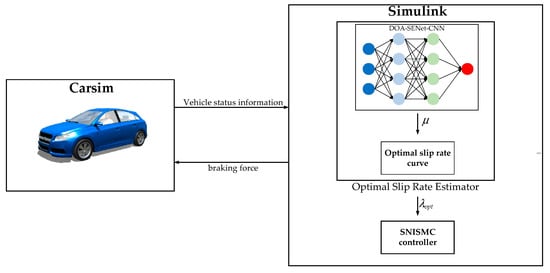
Figure 10.
Control system structure.
5.2. Experimental Results of Road Adhesion Coefficient Estimation
CarSim 2020 simulation software and Simulink are used to simulate the braking condition of the vehicle. The relevant state quantities , , , and of the vehicle during braking are used as the characteristic quantities of the neural network, where is the current slip ratio of the vehicle, is the current acceleration of the vehicle, is the vertical load of the wheel, and is the longitudinal force of the wheel. In the actual vehicle braking process, the optimal wheel slip ratio range is generally between 0.05 and 0.2. The data with a slip ratio interval of 0.2–1 on different roads have low values and overlap features, while the data with a slip ratio interval of from 0.02 to 0.2 have obvious features. Therefore, the data are preprocessed to leave only the characteristic data with a slip ratio between 0.05 and 0.2 to improve the training accuracy.
In the CarSim 2020 simulation software, configure the starting speed of the vehicle to 60 km/h, adjust the road adhesion coefficient between 0.05 and 1.2, and gather vehicle data through Simulink. The collected data are trained by the CDOA-SENet-CNN neural network, the feedforward neural network based on the Levenberg–Marquardt algorithm (LM-FNN) [27], BP neural network, and Elman neural network [28]. The training evaluation indicators include the determination coefficient , mean absolute error , root mean square error , mean square error , and mean absolute percentage error . The training outcomes of the BP neural network appear in Figure 11, the Elman neural network’s training outcomes are presented in Figure 12; the training results of LM-FNN are presented in Figure 13 and the training outcomes of the CDOA-SENet-CNN neural network are illustrated in Figure 14.
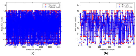
Figure 11.
The effect of BP neural network: (a) training set prediction results; (b) test set prediction results.
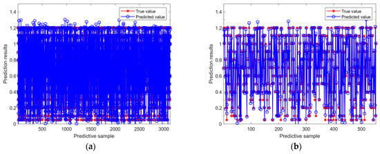
Figure 12.
The effect of the Elman neural network: (a) training set prediction results; (b) test set prediction results.
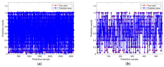
Figure 13.
The effect of the LM-FNN neural network: (a) training set prediction results; (b) test set prediction results.
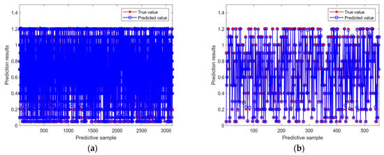
Figure 14.
The effect of the CDOA-SENet-CNN neural network: (a) training set prediction results; (b) test set prediction results.
It can be seen from Table 6 that the training effect of the CDOA-SENet-CNN neural network is better than other neural networks and can be capable of precisely determining the peak adhesion coefficient of the present road.
Table 6.
Performance comparison.
5.3. Simulation of ABS Control System
To evaluate the robustness of single-neuron sliding mode control, a simulation environment was built using CarSim 2020 and MATLAB/Simulink R2024b. The vehicle’s initial speed was 60 km/h on a flat, obstacle-free road. Two road conditions were set: one with a variable adhesion coefficient to mimic sudden changes during braking, and another with a constant adhesion coefficient. These conditions were aimed at assessing the single neuron sliding mode control’s performance under different adhesion scenarios.
In the case of a constant adhesion coefficient road, assuming the vehicle’s starting speed is 60 km/h, the road is 100 m long, and the maximum adhesion coefficient of the road is 0.8, the CarSim 2020 road simulation environment diagram is shown in Figure 15.
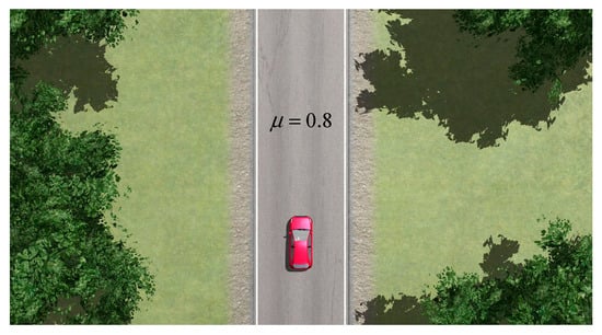
Figure 15.
Constant adhesion coefficient road simulation.
The adjustment time is the time when the control system achieves its steady-state value within the error range of , when the simulated road adhesion coefficient is constant, as presented in Figure 16a. When SMC control is adopted, it enters the steady state at t = 0.00608, the overshoot is 26.23%, and the error is 0.0005. When the control strategy adopts Super-Twisting Sliding Mode Control (STSMC), the system wheel slip ratio enters the steady state at t = 0.00183, the overshoot is 2.02%, and the error is 0.000021. When the control strategy adopts Fuzzy Sliding Mode Control (FSMC), the system wheel slip ratio enters the steady state at t = 0.00221, the overshoot is 8.33%, and the error is 0.000046. When SNISMC control is adopted, it enters the steady state at t = 0.002, the overshoot is 0%, and the error is 0.00003.
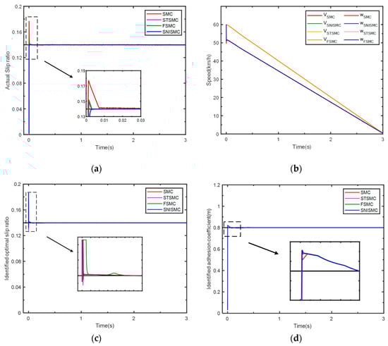
Figure 16.
Simulation results for roads with adhesion coefficient 0.8: (a) contrast between actual and estimated slip ratios; (b) comparison between vehicle and wheel speeds; (c) estimated slip ratio vs. actual optimal slip ratio; (d) actual vs. estimated road adhesion coefficients.
As shown in Table 7, SMC achieves rapid tracking of the system setpoint but suffers from large overshoot and large chatter. STSMC and FSMC reduce chatter and overshoot to a certain extent. SNISMC achieves rapid tracking and significantly reduces overshoot and chatter.
Table 7.
The control performance of the road surface with an adhesion coefficient of 0.8.
In actual urban roads, asphalt pavements are often sprayed with water to clean dust to extend their service life. This process will put the pavement in a medium-wet state. However, due to uneven watering or differences in the condition of the pavement itself, some areas may be smoother than other areas, similar to wet concrete surfaces, resulting in changes in the adhesion coefficient. To validate the robustness of SNISMC control when the adhesion coefficient changes abruptly, this paper selected medium-wet asphalt and wet concrete pavements of real urban roads as the test environment and set the pavement conditions where the adhesion coefficient suddenly changes from 0.8 to 0.5 to cover most of the sudden changes in the adhesion coefficient of real roads. Specifically, the initial vehicle speed is established at 60 km/h, and the total length of the test pavement is 100 m. The maximum adhesion coefficient of the 0–15 m section is 0.8, corresponding to the medium-wet asphalt pavement; the 15–100 m section has a maximum adhesion coefficient of 0.5, corresponding to the wet concrete pavement. This setting is intended to simulate the sudden changes in the pavement adhesion coefficient that vehicles may encounter in actual driving. The CarSim 2020 pavement simulation environment is shown in Figure 17.
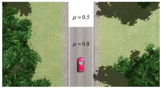
Figure 17.
Simulation of constant adhesion coefficient road.
According to Figure 18a, the maximum adhesion coefficient is 0.8 when the vehicle commences braking, and the braking effect is the same as on a road with a constant adhesion coefficient of 0.8. At t = 1.65262, the road adhesion coefficient suddenly changes to 0.5. The SMC enters a steady state at t = 1.65874 with an error of 0.000425. The STSMC enters a steady state at t = 1.65865 with an error of 0.000089. The FSMC enters a steady state at t = 1.65827 with an error of 0.00011. The SNISMC enters a steady state at t = 1.65379 with an error of 0.000077.
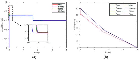
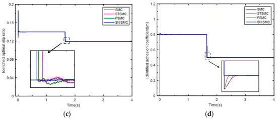
Figure 18.
Simulation of roads with adhesion coefficients of 0.5–0.8: (a) contrast between actual and estimated slip ratios; (b) vehicle and wheel speed comparison; (c) estimated vs. actual optimal slip ratio analysis; (d) actual and estimated road adhesion coefficient comparison.
As shown in Table 8, SMC can follow the optimal slip rate, but it has a slow response speed and exhibits significant vibration during steady-state conditions, which is detrimental to stable control during vehicle braking. Both STSMC and FSMC can reduce vibration to some extent, but they also have slow response speeds. In contrast, SMC can quickly follow changes and exhibits minimal vibration. This outcome thus confirms the efficacy and robustness of our proposed method.
Table 8.
The control performance on the pavement featuring an adhesion coefficient ranging from 0.8 to 0.5.
6. Discussion
In terms of identifying peak road adhesion coefficients, the CDOA-SENet-CNN method has advantages such as fast identification speed, high accuracy, and strong ability to explore unknown roads compared with Elman neural network estimation, fuzzy algorithm estimation, and online model identification. In terms of optimal slip ratio control, the SISMC control strategy designed in this paper has certain advantages over existing slip ratio control strategies (such as SMC, STSMC, and FSMC) in terms of response speed, vibration reduction, and overshoot reduction. In theory, the CDOA-SENet-CNN fusion model enriches the intelligent estimation system of road adhesion coefficient; the SNISMC strategy uses a single neuron to adaptively adjust the sliding mode approach law, providing a new solution with low jitter and strong anti-disturbance for anti-skid control. In practice, this method can shorten the vehicle braking distance and improve driving safety.
Based on the above discussion, for vehicle manufacturers, CDOA-SENet-CNN can be embedded in the vehicle control unit (VCU) to achieve online peak adhesion coefficient estimation through offline training and utilize SNISMC to adjust the brake cylinder pressure in real time, thereby shortening the braking distance and meeting ASIL-C functional safety requirements. For brake system suppliers, SNISMC can replace existing PID controllers after testing to improve system robustness under complex road conditions.
In addition, since sensors are susceptible to interference in actual applications, the collected data may contain noise, which may affect the estimation results. Future research can explore the use of noise reduction methods or data processing algorithms to reduce the impact of noise on the estimation. At the same time, this study will continue to consider the braking conditions under vehicle deviation conditions in the future.
7. Conclusions
This paper makes a key advancement by presenting a CDOA-SENet-CNN neural network approach for optimal slip ratio estimation. This method swiftly determines the optimal slip ratio at the start of braking and, combined with SNISMC control, obtains the minimal stopping distance by utilizing the ideal slip ratio. When contrasted with current techniques, the CDOA-SENet-CNN neural network can accurately explore the optimal slip ratio under unknown road conditions. SNISMC enhances the control system’s anti-interference and robustness compared to traditional algorithms. The principal findings are as follows:
- (1)
- The optimal slip ratio estimator collects vehicle data from diverse road conditions. The trained neural network boosts the estimation precision for unknown road conditions.
- (2)
- This paper proposes a single-neuron-based integral sliding mode control strategy featuring high precision, fast convergence, and strong robustness. Its high anti-interference ability reduces chattering and improves stability.
- (3)
- Through creating a variable adhesion coefficient road surface, the effectiveness and stability of SNISMC control are verified, enhancing vehicle safety during emergency braking.
Author Contributions
Conceptualization, Y.W. and W.H.; methodology, Y.W.; software, Y.W.; validation, X.H. and Y.Z.; data curation, Y.X.; investigation, Y.G.; resources, Y.C.; writing—original draft preparation, Y.W.; writing—review and editing, Y.W.; project administration, Y.W. All authors have read and agreed to the published version of the manuscript.
Funding
This research received no external funding.
Data Availability Statement
The original contributions presented in this study are included in the article. Further inquiries can be directed to the corresponding author.
Conflicts of Interest
The authors declare no conflicts of interest.
References
- Vošahlík, D.; Hanis, T. Real-time estimation of the optimal longitudinal slip ratio for attaining the maximum traction force. Control Eng. Pract. 2024, 145, 105876. [Google Scholar] [CrossRef]
- Chen, L.; He, Y.; Ma, T.; Zhong, S. Online Estimation and Control Method of Optimal Slip Ratio for Vehicle with an Electric Power-Assisted Brake System. IEEE Access 2024, 12, 176961–176981. [Google Scholar] [CrossRef]
- Liu, J.; Zhang, Y.; Liu, J.; Wang, Z.; Zhang, Z. Automated Recognition of Snow-Covered and Icy Road Surfaces Based on T-Net of Mount Tianshan. Remote Sens. 2024, 16, 3727. [Google Scholar] [CrossRef]
- Xu, Z.; Wang, J.; Lu, Y.; Li, H. Estimation Strategy for the Adhesion Coefficient of Arbitrary Pavements Based on an Optimal Adaptive Fusion Algorithm. Machines 2024, 13, 17. [Google Scholar] [CrossRef]
- Vieira, D.; Orjuela, R.; Spisser, M.; Basset, M. An adapted Burckhardt tire model for off-road vehicle applications. J. Terramechanics 2022, 104, 15–24. [Google Scholar] [CrossRef]
- Bakker, E.; Nyborg, L.; Pacejka, H.B. Tyre modelling for use in vehicle dynamics studies. SAE Trans. 1987, 96, 190–204. [Google Scholar]
- Ulsoy, A.G.; Peng, H.; Çakmakci, M. Automotive Control Systems; Cambridge University Press: Cambridge, UK, 2012. [Google Scholar]
- Chen, Y.-H. Nonlinear Adaptive Fuzzy Hybrid Sliding Mode Control Design for Trajectory Tracking of Autonomous Mobile Robots. Mathematics 2025, 13, 1329. [Google Scholar] [CrossRef]
- Xu, G.; Zhao, S.; Cheng, Y. Chaotic synchronization based on improved global nonlinear integral sliding mode control. Comput. Electr. Eng. 2021, 96, 107497. [Google Scholar] [CrossRef]
- Sun, X.; Xiao, Z.; Wang, Z.; Zhang, X.; Fan, J. Acceleration Slip Regulation Control Method for Distributed Electric Drive Vehicles under Icy and Snowy Road Conditions. Appl. Sci. 2024, 14, 6803. [Google Scholar] [CrossRef]
- Zhang, J.; Sun, W.; Jing, H. Nonlinear robust control of antilock braking systems assisted by active suspensions for automobile. IEEE Trans. Control Syst. Technol. 2018, 27, 1352–1359. [Google Scholar] [CrossRef]
- Shen, Y.; Mao, J.; Wu, A.; Liu, R.; Zhang, K. Optimal slip ratio tracking integral sliding mode control for an EMB system based on convolutional neural network online road surface identification. Electronics 2022, 11, 1826. [Google Scholar] [CrossRef]
- Guan, H.; Wang, B.; Lu, P.; Xu, L. Identification of maximum road friction coefficient and optimal slip ratio based on road type recognition. Chin. J. Mech. Eng. 2014, 27, 1018–1102. [Google Scholar] [CrossRef]
- Luo, S.; Zhang, B.; Ma, J.; Zheng, X. Research on a Hierarchical Control Strategy for Anti-Lock Braking Systems Based on Active Disturbance Rejection Control (ADRC). Appl. Sci. 2025, 15, 1294. [Google Scholar] [CrossRef]
- He, Z.; Shi, Q.; Wei, Y.; Gao, B.; Zhu, B.; He, L. A model predictive control approach with slip ratio estimation for electric motor antilock braking of battery electric vehicle. IEEE Trans. Ind. Electron. 2021, 69, 9225–9234. [Google Scholar] [CrossRef]
- Zhang, H.; Qi, Y.; Si, W.; Zhang, C. An Improved Adaptive Sliding Mode Control Approach for Anti-Slip Regulation of Electric Vehicles Based on Optimal Slip Ratio. Machines 2024, 12, 769. [Google Scholar] [CrossRef]
- Kanungo, A.; Kumar, P.; Gupta, V.; Salim; Saxena, N.K. A design an optimized fuzzy adaptive proportional-integral-derivative controller for anti-lock braking systems. Eng. Appl. Artif. Intell. 2024, 133, 108556. [Google Scholar] [CrossRef]
- Zhou, H.; Liu, W.; Wang, R.; Ding, R.; Guo, Z.; Ye, Q.; Meng, X.; Sun, D.; Liu, W. Anti-Lock Braking System Performance Optimization Based on Fitted-Curve Road-Surface Recognition and Sliding-Mode Variable-Structure Control. World Electr. Veh. J. 2025, 16, 156. [Google Scholar] [CrossRef]
- Güleryüz, I.C.; Başer, Ö. Modelling the longitudinal braking dynamics for heavy-duty vehicles. Proc. Inst. Mech. Eng. D J. Automob. Eng. 2021, 235, 2802–2817. [Google Scholar] [CrossRef]
- Yi, H.; Ke, Z.; Zou, J.; Shi, J.; Deng, Z. Nonlinear model predictive control for longitudinal tracking of maglev cars. J. Intell. Syst. Control 2024, 3, 42–56. [Google Scholar] [CrossRef]
- Li, Z.; Liu, F.; Yang, W.; Peng, S.; Zhou, J. A survey of convolutional neural networks: Analysis, applications, and prospects. IEEE Trans. Neural Netw. Learn. Syst. 2021, 33, 6999–7019. [Google Scholar] [CrossRef]
- Hu, J.; Shen, L.; Sun, G.; Wu, E. Squeeze-and-excitation networks. IEEE Trans. Pattern Anal. Mach. Intell. 2020, 42, 2011–2023. [Google Scholar] [CrossRef] [PubMed]
- You, X.; Zheng, Z.; Yang, K.; Yu, L.; Liu, J.; Chen, J.; Lu, X.; Guo, S. A PSO-CNN-based deep learning model for predicting forest fire risk on a national scale. Forests 2023, 15, 86. [Google Scholar] [CrossRef]
- Li, J.; Yang, D.; Guo, C.; Ji, C.; Jin, Y.; Sun, H.; Zhao, Q. Application of GPR system with convolutional neural network algorithm based on attention mechanism to oil pipeline leakage detection. Front. Earth Sci. 2022, 10, 863730. [Google Scholar] [CrossRef]
- Lang, Y.; Gao, Y. Dream Optimization Algorithm (DOA): A novel metaheuristic optimization algorithm inspired by human dreams and its applications to real-world engineering problems. Comput. Methods Appl. Mech. Eng. 2025, 436, 117718. [Google Scholar] [CrossRef]
- Utkin, V. Variable structure systems with sliding modes. IEEE Trans. Autom. Control. 2003, 22, 212–222. [Google Scholar] [CrossRef]
- Yadav, A.; Chithaluru, P.; Singh, A.; Joshi, D.; Elkamchouchi, D.H.; Pérez-Oleaga, C.M.; Anand, D. An enhanced feed-forward back propagation Levenberg–Marquardt algorithm for suspended sediment yield modeling. Water 2022, 14, 3714. [Google Scholar] [CrossRef]
- Wu, W.G.; Zhang, F.H.; Xu, M.L. Identification of road friction coefficient based on Elman neural network. J. Chongqing Univ. 2023, 46, 118–128. [Google Scholar]


Disclaimer/Publisher’s Note: The statements, opinions and data contained in all publications are solely those of the individual author(s) and contributor(s) and not of MDPI and/or the editor(s). MDPI and/or the editor(s) disclaim responsibility for any injury to people or property resulting from any ideas, methods, instructions or products referred to in the content. |
© 2025 by the authors. Licensee MDPI, Basel, Switzerland. This article is an open access article distributed under the terms and conditions of the Creative Commons Attribution (CC BY) license (https://creativecommons.org/licenses/by/4.0/).