1. Introduction
Diagnosing gear faults is crucial for maintaining machinery and ensuring its reliability [
1]. Gears are vital in mechanical systems, transmitting power and motion, which makes accurate fault diagnosis essential [
2,
3]. Their significant role in mechanical failures under various operating conditions further emphasizes this need [
4]. Undetected gear faults may trigger further failures throughout the transmission system. However, most current diagnostic approaches are designed for stationary operation conditions, and there is a notable lack of practical tools for identifying gear faults under non-stationary conditions with fluctuating loads and speeds [
5]. Gearboxes are among the most essential mechanical components in rotating machinery, playing a vital role in power transmission and overall system efficiency [
6,
7]. However, these components are frequently subjected to varying load conditions, changing rotational speeds, and harsh environmental factors, making them particularly vulnerable to faults and degradation [
8,
9]. Gearbox failures often result in extensive maintenance requirements, unexpected downtime, safety hazards, and even secondary failures in adjacent mechanical components [
10,
11]. Gearbox failures in real-world applications such as wind turbines, heavy-duty robotics, and automated manufacturing lines can spread through networked systems, resulting in cascading downtime across whole operations. Detecting even a little gear degradation across diverse speed profiles is crucial for condition-based maintenance and operational safety. These operational considerations highlight the significance of developing effective, responsive, and accurate fault diagnostic devices that can operate independently in non-stationary contexts.
Non-stationary vibration signals, often encountered during start-up, shutdown, load variation, or speed ramping, are notoriously difficult to analyze using conventional signal processing techniques [
12,
13,
14]. Traditional frequency-domain methods, such as the Fourier Transform (FT) [
15,
16], rely on the assumption of signal stationarity and thus fail to capture the temporal evolution of fault characteristics. While time-domain statistical features and envelope analysis remain widely used, they often lack robustness under variable-speed conditions [
17,
18]. They may not offer sufficient resolution to detect early-stage or compound faults. Furthermore, non-stationary vibration signals frequently comprise short-lived transient bursts, frequency modulations, and mode interactions that are suppressed under linear or globally stationary [
19,
20]. Thus, successful diagnostics necessitate time–frequency resolution, tolerance to temporal energy fluctuations, and structure-aware signal encoding.
Time–frequency analysis (TFA) [
21,
22] has emerged as a robust framework for characterizing non-stationary signals to address these challenges. Classical approaches such as the Short-Time Fourier Transform (STFT) [
23] and Continuous Wavelet Transform (CWT) [
24,
25] provide joint representations of time and frequency, allowing for the identification of transient or modulated signal components. However, both techniques have intrinsic limitations that hinder their applicability in complex scenarios. STFT uses a fixed-size window, which forces a compromise between time and frequency resolution. This limitation makes it unsuitable for signals with multiple frequency components that evolve at different rates. On the other hand, CWT offers a scale-adaptive decomposition, which improves multiresolution analysis but often results in energy smearing, poor localization of rapidly varying components, and difficulty in reconstructing the original signal.
To overcome the resolution trade-offs of classical techniques, reassignment methods such as the reassigned spectrogram and synchrosqueezing transforms (SST) [
26,
27,
28,
29] were developed. These methods reallocate energy in the time–frequency plane to reflect the instantaneous frequency content more accurately. SST, in particular, preserves the invertibility of the transformation, enabling improved signal reconstruction and more precise separation of overlapping modes. Among these, the Fourier-based Synchrosqueezing Transform (FSST) [
27] stands out due to its ability to sharpen spectral representations without departing from the Fourier framework, making it suitable for mechanical fault detection. Furthermore, high-order variants such as High-Order Synchrosqueezing Tranforms [
30,
31] offer additional benefits in capturing closely spaced components and improving resistance to noise. Despite their strong analytical performance, high-resolution TFA methods like FSST are computationally demanding. Their reliance on dense time-frequency grids and exhaustive reassignment operations poses a significant challenge for processing long-duration signals or implementing real-time diagnostics in embedded systems. The trade-off between diagnostic resolution and computational cost becomes increasingly pronounced in practical industrial environments, where hundreds of machines might be monitored simultaneously. Moreover, hardware limitations can further constrain high-resolution TFA methods, especially in edge devices or low-power industrial controllers. While modern computational architectures can support deep learning-based fault classification, the high dimensionality and memory consumption of traditional time–frequency representations can still hinder deployment at scale. Therefore, there is a clear need for TFA methods that maintain diagnostic fidelity while reducing computational complexity and memory footprint.
A novel data-driven framework for gearbox fault diagnostics under non-stationary conditions is needed to bridge the gap between analytical robustness and operational scalability. Central to this framework is the Data-Driven Synchrosqueezing-based Signal Transformation (DSST)—a lightweight, scalable, and resolution-preserving method that integrates synchrosqueezing theory with structured downsampling strategies. The DSST algorithm is designed to retain the high-resolution characteristics of SST while minimizing computational overhead, enabling its integration into real-time monitoring systems and machine learning-based diagnostic pipelines. The DSST framework addresses key weaknesses in existing TFA methods through two main innovations. First, it retains the precision of SST in concentrating spectral energy along instantaneous frequency ridges, thereby preserving fault-sensitive information even in the presence of transient and overlapping components. Second, it introduces principled downsampling in both time and frequency domains to reduce the size of the time-frequency matrix, focusing computational resources on signal regions that carry the most relevant diagnostic information.
Recent studies have attempted to reduce the computational load of synchrosqueezing by incorporating downsampling strategies. For instance, a downsampling-based SST [
32] was proposed to accelerate time–frequency analysis in large-scale vibration datasets, demonstrating significant reductions in processing time while preserving critical diagnostic features. Although it offers significant improvements in computational efficiency, it remains limited in terms of practical applicability to real-world diagnostics. The method primarily prioritizes algorithmic formulation and mathematical efficiency, without addressing interpretability, real-time deployment, or integration into data-driven diagnostic systems. It does not demonstrate signal reconstruction in an industrial context, nor does it extract fault-specific features such as gear meshing frequency (GMF) harmonics or sidebands from actual vibration data. This study overcomes the limitations of that work by proposing a Data-Driven Synchrosqueezing-based Signal Transformation (DSST), which retains the high-resolution properties of SST while introducing structured downsampling and reconstruction strategies tailored for gearbox fault diagnosis under non-stationary conditions. Unlike previous approaches, DSST is formulated as an interpretable and scalable diagnostic module that is compatible with machine learning frameworks and suitable for peripheral deployment in modern condition monitoring systems.
In contrast, the proposed framework in this work extends beyond computational efficiency. It incorporates structured sparsity in both time and frequency dimensions, maintains invertibility for signal reconstruction, and is specifically designed to output compact, interpretable features that can be directly integrated into data-driven diagnostic models. Furthermore, DSST is formulated as part of a broader fault diagnostic pipeline, explicitly targeting rotating machinery operating under non-stationary conditions, emphasizing edge-deployable and learning-friendly representations.
Furthermore, the invertibility of DSST enables it to serve as a foundational component of hybrid frameworks that combine interpretability and automation. By allowing signal reconstruction from its sparse representation, the technique aids applications that require explainability and traceability, such as in safety-critical or regulated situations. It also enables effective storage and transfer of diagnostic data across remote systems. The modular design of DSST allows smooth integration into multimodal condition monitoring architectures. Its tiny outputs can be used as low-latency input for learning-based anomaly detectors or combined with data from other sources, such as acoustic emissions or motor current signals, to improve diagnostic accuracy. From a broader perspective, the proposed DSST is consistent with the growing demand for edge-compatible fault diagnosis systems in Industry 4.0 environments. The lower computing load of DSST makes it easier to implement on embedded platforms and supports predictive maintenance scenarios that require rapid judgments. The method’s compliance with real-time inference makes it more suitable for closed-loop control systems, where fault identification must be quick and less invasive.
To summarize, the DSST algorithm combines theoretical rigor and technical applicability. It retains the analytical advantages of synchrosqueezing, while resolving the limitations that prevent high-resolution TFA approaches from scaling to industrial-scale installations. Compared to existing works that treat downsampled SST as a standalone signal processing method, DSST is framed as a cohesive diagnostic module within a broader data-driven framework. This architectural distinction ensures compatibility with emerging intelligent monitoring systems that demand computational efficiency and traceable and machine-interpretable features. Finally, DSST fills a significant gap in the field: balancing analytical integrity with computing feasibility. As industrial systems grow in complexity and data volume, lightweight yet exact approaches will become increasingly crucial for providing rapid, interpretable, and autonomous problem diagnostics.
The remainder of this paper is organized as follows:
Section 2 presents the mathematical foundation of synchrosqueezing and details the formulation of the DSST algorithm, including downsampling principles and reconstruction capabilities.
Section 3 presents the experimental setup, and the datasets used for validation, followed by the benchmarking protocols and evaluation metrics. It then discusses the obtained results, emphasizing the diagnostic accuracy of DSST, its computational efficiency, and its applicability to non-stationary operating conditions. Finally,
Section 4 concludes the paper with insights on limitations, industrial deployment considerations, and avenues for future research, including adaptive resolution control, hybrid learning-based frameworks, and multi-source signal fusion.
2. Methodology
To effectively analyze non-stationary vibration signals under varying operating conditions, a combination of classical time-frequency methods and a novel downsampling-based synchrosqueezing approach is employed. The methodology focuses on improving time–frequency resolution while maintaining computational efficiency for large-scale diagnostic applications.
2.1. Short-Time Fourier Transform
STFT is a powerful tool for analyzing non-stationary signals, allowing for simultaneous analysis in both time and frequency domains [
33]. This is achieved by dividing the signal into short segments and applying the Fourier transform to each segment, capturing the time-varying frequency content of the signal.
where
is the STFT of the signal
,
is the signal being analyzed,
is a window function, and
represents the complex exponential basis functions used in the Fourier transform [
34].
For practical applications involving discrete signals, the discrete form of the STFT is described as follows [
34]
where
is the discrete signal,
is the discrete window function,
is the frequency bin index, and
is the number of points in the Fourier transform.
One of the main concepts in STFT is the trade-off between time resolution (
) and frequency resolution
. This is governed by the Heisenberg Uncertainty Principle in signal processing:
This inequality establishes a strict limitation: improving time resolution results in a degradation of frequency resolution, and vice versa. The choice of window length directly influences this balance:
Short Window (High Time Resolution): A short analysis window provides precise localization in time, allowing the detection of transient events or rapid changes in the signal. However, the shorter the window, the broader its frequency spectrum, leading to poorer frequency resolution.
Long Window (High Frequency Resolution): A longer analysis window sharpens the frequency resolution, making it suitable for identifying stable or harmonic frequency components. However, this improvement comes at the expense of reduced time resolution, as the window spans over longer periods, blurring rapid time-domain events.
The spectrogram is one of the most common tools used to visualize the results of the STFT. It represents the time-varying frequency content of a signal by plotting the magnitude of the STFT squared
where
is the STFT of the signal, computed using a window function
,
represents time,
denotes frequency, and
corresponds to the power or energy at a specific time
and frequency
.
2.2. Fourier-Based Synchrosqueezing Transform
FSST is an advanced signal analysis technique that enhances the Time-Frequency (TF) resolution compared to traditional STFT. By more accurately adjusting the frequency components, FSST provides a clearer and more detailed representation of a signal’s structure, making it particularly useful for analyzing complex and non-stationary signals where precise TF localization is crucial [
35,
36].
The instantaneous frequency of the signal at time
t and frequency
f is calculated as
To apply the FSST effectively, certain specific conditions must first be satisfied for a multicomponent signal (MCS). These conditions ensure that the signal is well suited for precise time-frequency analysis and that the synchrosqueezing process can achieve its intended goal of energy reassignment with high accuracy.
The first condition for applying FSST is that the amplitude
must be continuously differentiable
) and bounded
). It must also be strictly positive:
Additionally, the amplitude must vary slowly over time, satisfying
The second condition concerns the phase
of each signal component. The phase must be twice continuously differentiable
) to ensure smooth and gradual variations. Its first derivative, representing the instantaneous frequency, must always be positive and bounded:
Additionally, the second derivative of the phase,
, which indicates the rate of change in the instantaneous frequency, must also vary slowly:
The final condition ensures that the frequency separation between adjacent components is sufficiently large to avoid overlapping. Specifically, the difference between the instantaneous frequencies of consecutive components must satisfy the following:
Using threshold
γ and accuracy
λ, the FSST of
f is defined by [
35]
If
λ and
γ approach zero,
converges to a specific value, which we formally express as
referred to as FSST in the following, where
δ denotes the Dirac distribution.
2.3. Downsampled Discrete STFT
The Downsampled Discrete STFT improves computational efficiency by combining downsampling factors
and frequency downsampling factors
. This technique is particularly suitable for analyzing large-scale vibration signals while maintaining the essential features of TF analysis [
32].
where
m and
k are time and frequency sequence,
and
are the two downsampling factors, and N is the sampling point.
For practical implementation, assuming that the discrete window
is consistent for every step and has a support range of
, the convolution simplifies into the form of a Discrete Fourier Transform (DFT)
where
.
To simultaneously enhance the frequency resolution while maintaining computational efficiency, the number of DFT points,
, is chosen so that
This results in the refined formulation:
Furthermore, the computation of the DFT in Equation (16) can be accelerated by selecting as a power of 2, enabling the use of the FFT algorithm.
2.4. Reassignment Method
The reassignment method (RM) aims to enhance the clarity of TF representations by repositioning calculated values to improve the concentration of signal components, thereby reducing misleading interference terms [
37]. This improves the accuracy of analyzing and classifying non-stationary signals [
38]. Reassignment parameters are calculated as follows:
First, we calculate the reassignment parameters:
The STFT
is reassigned to a new position
using these reassignment parameters
where
is the spectrogram of STFT and
denotes the Dirac impulse.
The reassignment process addresses the poor time–frequency concentration of the spectrogram by redistributing energy to more accurate locations. In a standard spectrogram, signal energy is often dispersed, making key components hard to identify due to the inseparable kernel of STFT. Reassignment corrects this by relocating energy to its true instantaneous frequency and time, resulting in sharper and more precise time-frequency representations, particularly for analyzing non-stationary signals.
2.5. Downsampled Synchrosqueezing Transform
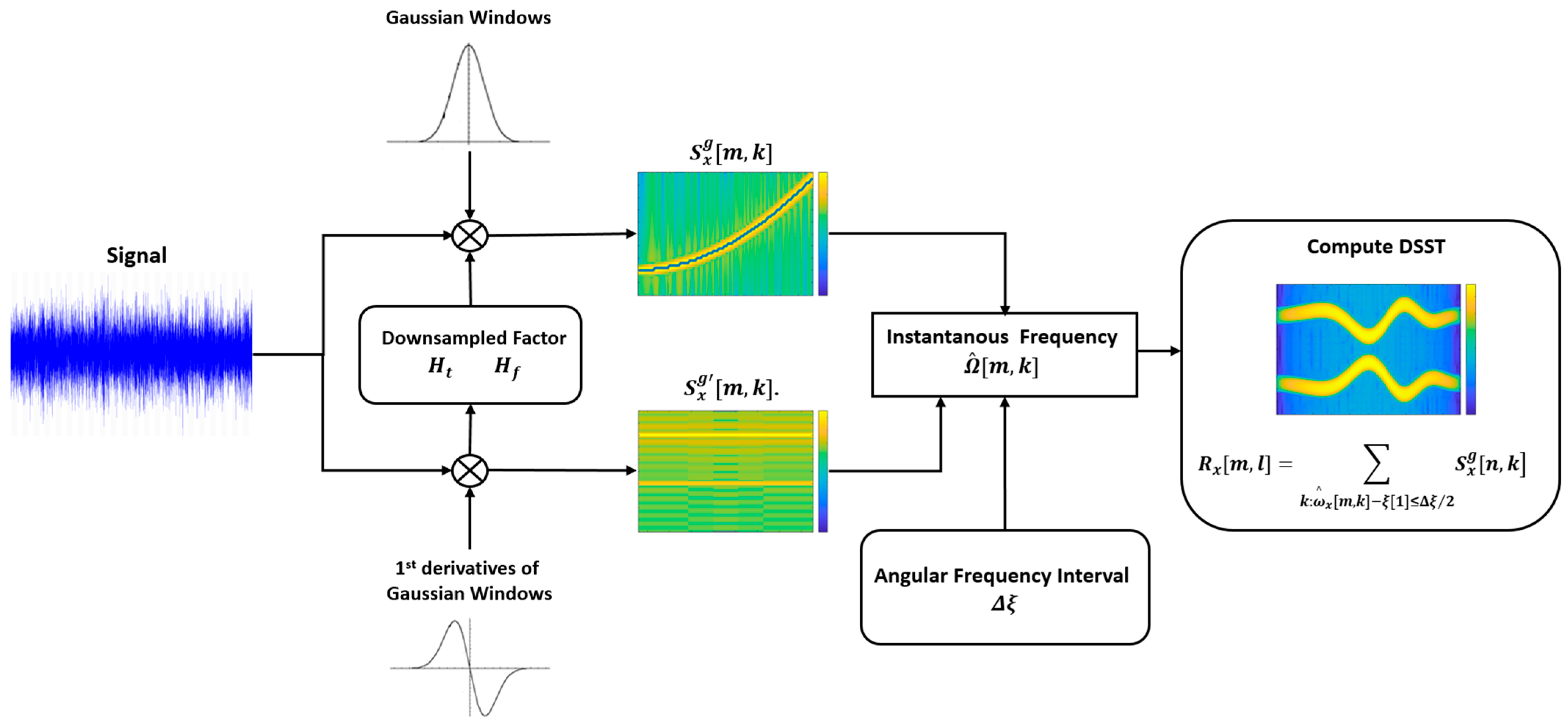
To clearly outline the steps of DSST,
Figure 1 will be designed as a flowchart detailing each phase of the proposed approach.
The DSST process begins with the application of two different window functions, and , where is sampled from , to the input signal . These windowed signals are then convolved with the input signal and subsequently downsampled by factors and . The downsampled signals are used to compute the STFT, represented as and .
In the reassignment process, the discrete instantaneous frequency (IF) estimator
for the signal
is calculated using the angular frequency interval
, expressed as
where
is the discrete angular frequency sequence for
.
The estimator
is derived by combining the two STFTs
and
as follows
where
represents the imaginary part, and
is the threshold.
This method ensures precise reassignment of time–frequency energy by accurately estimating the instantaneous frequency.
The final reassignment step involves computing the reassigned STFT result by reallocating the TF coefficients based on the estimated instantaneous frequency. This process enhances the readability and accuracy of the TF representation of the signal.
3. Results and Discussion
To validate the proposed method, experimental data from a group at Tsinghua University was utilized [
39]. The vibration signal collection process spans 40 s. Initially, the shaft speed is 3000 RPM for 10 s, then it decreases to 2500 RPM over the next 5 s, remains constant for 10 s, increases back to 3000 RPM in 5 s, and remains stable for the final 10 s (
Figure 2). The accelerometer’s sampling frequency is set at 12,800 Hz, and the electromagnetic brake load is fixed at 2 Nm.
Figure 3 illustrates the spectrograms corresponding to four distinct gear conditions: healthy gear, gear pitting, missing teeth, and broken teeth. These spectrograms, derived using MATLAB’s Short-Time Fourier Transform, depict the time-varying frequency content of vibration signals collected over a 40 s window. As seen in all four cases, the gear mesh frequency (GMF) is not constant but changes over time, reflecting the non-stationary nature of the rotating system due to variations in shaft speed. This observation underscores the need for high-resolution time–frequency analysis techniques that are not only capable of accurately tracking time-varying spectral components but also efficient enough to process large-scale vibration data collected over extended monitoring periods.
While the GMF remains visually prominent, the spectrogram fails to resolve finer structures, particularly the sidebands associated with localized gear faults. In the gear pitting and teeth break conditions, these sidebands, critical for differentiating fault types, are only faintly visible or almost completely smeared. In the cases of missing or broken teeth, the differences in spectral behavior are subtle and hard to discern using the spectrogram alone.
This loss of diagnostic detail is a direct result of the STFT’s fixed window length, which imposes a trade-off between time and frequency resolution. When applied to long-duration signals with non-stationary content, the spectrogram distributes energy across broader frequency bands, making it difficult to isolate transient or overlapping components. As such, while spectrograms provide a general overview of frequency evolution, their limited resolution restricts their utility for precise fault classification under varying operational conditions.
Figure 4 presents the time–frequency spectra obtained using the FSST for the same vibration datasets. In contrast to the spectrogram results in
Figure 3, FSST provides a significantly sharper and more concentrated time–frequency representation. It successfully reveals both the gear mesh frequency (GMF) and its associated sidebands with greater clarity and continuity, especially in periods where rotational speed varies. These improvements directly address the limitations of STFT-based spectrograms, which suffer from energy smearing due to fixed window lengths and limited adaptability to non-stationary components. As such, FSST proves to be a powerful analytical tool for revealing transient and modulated features that are critical for fault diagnosis in rotating machinery.
However, this enhancement in diagnostic fidelity comes with considerable computational overhead. In practical implementation, generating a single FSST-based time–frequency spectrum for a 40 s vibration signal can take up to 60 min, even on a modern workstation. This prolonged processing time stems from FSST’s need to compute dense time–frequency grids and perform high-resolution reassignment operations across the entire frequency range. The algorithm must estimate instantaneous frequencies at each time-frequency bin and then reallocate energy accordingly—operations that are mathematically demanding and computationally intensive.
Moreover, FSST’s high memory consumption further restricts its usability in embedded or real-time systems. As the length of the input signal increases or higher resolution is required, memory demands grow exponentially, making the method unsuitable for deployment on edge devices or within scalable monitoring infrastructures that must handle hundreds of machines in parallel. Even in high-performance computing environments, the resource allocation required for FSST limits its applicability in continuous monitoring scenarios, where fast and responsive algorithms are essential.
This trade-off between time–frequency resolution and computational efficiency forms the core limitation of FSST in real-world applications. While it undoubtedly surpasses conventional spectrograms in its ability to resolve fine-grained fault features, the method’s excessive processing time and hardware dependency create a substantial barrier to its adoption in industry. In modern condition monitoring systems, especially those aligned with Industry 4.0 principles, methods must not only be accurate but also scalable, fast, and lightweight. The inability of FSST to meet these practical requirements highlights a critical need for alternative approaches that retain its diagnostic advantages while mitigating computational costs.
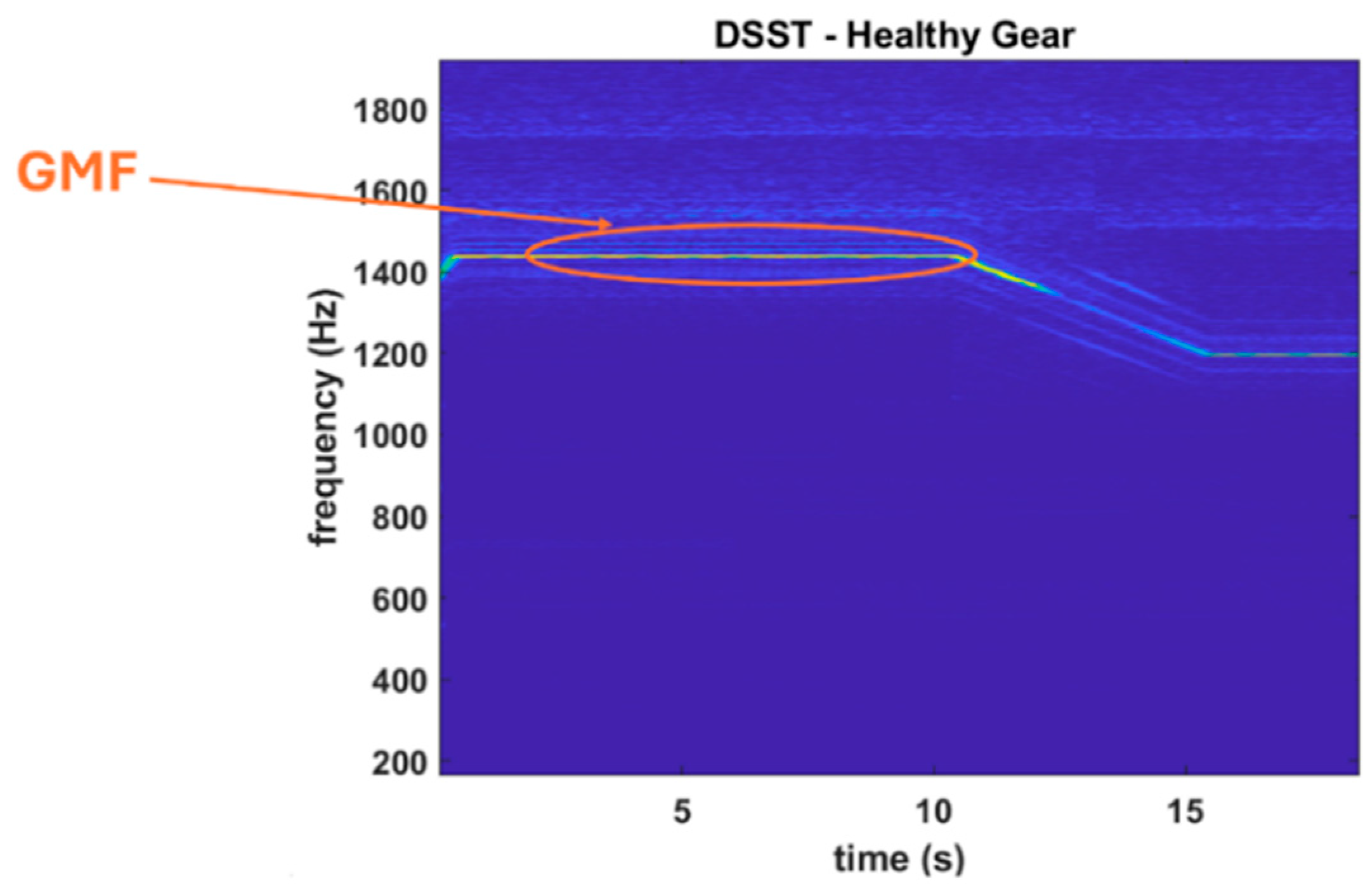
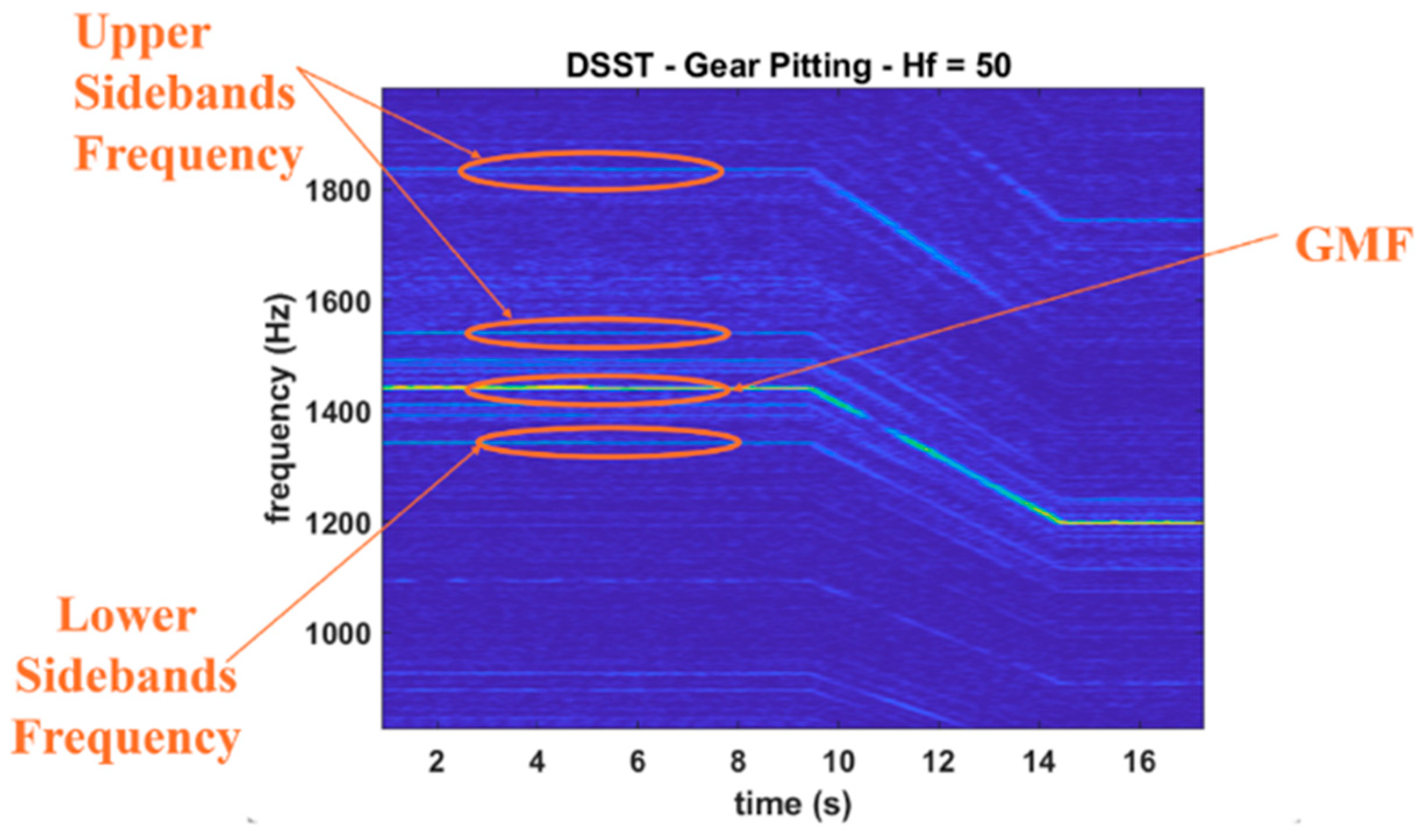
Figure 5a,b illustrates the time–frequency representations obtained using the proposed DSST method for the healthy and gear pitting conditions, respectively. A direct comparison with the results from FSST confirms that DSST maintains a comparable level of resolution, effectively preserving key diagnostic features such as the GMF and its sidebands throughout the duration of the signal. The spectral energy remains well localized, even under non-stationary operating conditions, highlighting the method’s robustness in tracking dynamic frequency variations. Most importantly, this level of diagnostic clarity is achieved with a drastically reduced computational burden. In contrast to FSST, which requires up to 60 min of processing time per dataset, DSST performs the full analysis in a matter of seconds. This efficiency stems from the structured downsampling strategy implemented in both time and frequency domains, which significantly reduces the size of the time–frequency matrix without sacrificing spectral fidelity. The method strategically focuses computational resources on the most informative regions of the signal, making it suitable for deployment in real-time systems and on resource-constrained platforms. The DSST results not only replicate the interpretability of FSST but also demonstrate enhanced practicality. In the gear pitting case (
Figure 5b), sidebands around the GMF are clearly distinguishable and sharply defined—an essential criterion for early and accurate fault classification. The method’s ability to preserve such features while dramatically reducing computation time underscores its superiority over existing high-resolution transforms. In summary, DSST achieves a critical balance between diagnostic resolution and processing efficiency. It provides a high-fidelity time–frequency representation necessary for fault identification, while enabling scalable, low-latency implementation suitable for modern industrial monitoring environments. These findings establish DSST as a significant advancement over prior approaches, addressing both the computational limitations of FSST and the interpretability shortcomings of traditional STFT-based methods.
To further substantiate the effectiveness of the proposed method,
Figure 6 and
Figure 7 provide magnified views of the time–frequency spectra previously shown in
Figure 5, focusing on representative fault cases. These zoomed-in visualizations allow for closer inspection of the spectral features associated with healthy and pitting gear conditions, revealing the diagnostic detail captured by DSST with improved clarity.
In
Figure 6, corresponding to the healthy gear case, the GMF is distinctly visible as a clean and continuous ridge without the presence of surrounding sidebands—an expected spectral signature in the absence of faults. This result confirms that DSST accurately preserves fundamental gear dynamics while avoiding false indications of damage. By contrast,
Figure 7 illustrates the gear pitting scenario and clearly exhibits multiple sidebands distributed both above and below the GMF. These spectral components are characteristic of amplitude and frequency modulations induced by localized tooth damage. The visibility of both upper and lower sidebands in the time–frequency plane underscores the method’s sensitivity to fault-induced modulations. Importantly, despite being visualized at a high time downsampling factor, the DSST results maintain sharp spectral concentration, demonstrating that critical diagnostic features are retained even under aggressive computational simplification. Together, these figures reinforce that DSST not only captures the essential fault-related features necessary for accurate diagnosis but does so in a computationally efficient manner. The method strikes a highly effective balance between spectral resolution and processing cost, enabling the reliable identification of gear faults under non-stationary conditions with minimal sacrifice in interpretability.
Figure 8 displays the results of the DSST transform applied to the gear pitting case with different time downsampling factors (
= 1, 20, 50), while keeping the frequency downsampling factor constant (
= 1). From a visual perspective, increasing
has minimal impact on the concentration or readability of the time–frequency representation (TFR). The GMF and its sidebands remain clearly identifiable across all cases, confirming that the diagnostic features are preserved.
However, computational efficiency improves significantly as increases. For example, with = 50, the processing time is drastically reduced compared to = 1, while maintaining comparable resolution. This demonstrates the effectiveness of DSST in balancing computational efficiency with diagnostic accuracy. Furthermore, when compared to SST, the DSST method provides similar TFR clarity, emphasizing its capability to process large-scale vibration data with reduced computational load.
However, the most significant difference is shown in
Table 1, where the elapsed time is considerably reduced compared to SST, 3.45 s, when
= 20 and 1.15 s when
= 50. The time cost in the second row is nearly half that of the first row, as the number of DFT points is halved. Similarly, the time cost in the second and third columns is about 1/20 and 1/50 of that in the first column, respectively. This demonstrates the efficiency of the proposed method in minimizing computational complexity while retaining the characteristic damage values.
Table 1 highlights the significant improvement in computational efficiency achieved by the DSST method with different time downsampling factors (
). When
= 1, the elapsed time is 60.45 s, equivalent to the computational time of SST. However, by increasing
to 20, the elapsed time reduces dramatically to 3.45 s, approximately 1/20 of the initial time. Further increasing
to 50 reduces the processing time to just 1.15 s, roughly 1/50 of the original duration.
This reduction in time is directly correlated with the number of DFT points processed, as increasing effectively decreases the size of the time-domain data. Despite this drastic reduction in computational load, the diagnostic capability of DSST remains intact, as shown in the previous figures. The method successfully retains critical features such as the GMF and sidebands, which are essential for fault diagnosis.
Figure 9 continues to illustrate the results of the DSST method with the gear pitting data when changing the
factor. The elapsed time of the algorithm continues to demonstrate the efficiency of the proposed method, with the SST transform taking up to 59.98 s to process, while the DSST transform with
takes 3.75 s and with
takes 1.27 s, as shown in
Table 2. However, unlike when changing the
coefficient, the resolution of TF representation is not significantly affected. When changing the
coefficient, the resolution decreases significantly. To quantitatively assess the impact of the downsampling factor on the concentration of TFR, particularly when using a relatively large factor, Rényi entropy is used. This entropy quantifies the concentration of the TFRs produced by fully sampled SST, downsampled SST, and STFT.
The Rényi entropy of order
α for a TFR
is described as [
40,
41]
For SST, the downsampling factors in the time and frequency domains influence concentration in distinct ways. The entropy of SST remains stable with changes in but rises significantly with increases in . This is because has a more substantial effect on SST concentration due to the reassignment of TF energy along the frequency axis.


 ,
, 


