Intelligent Effluent Management: AI-Based Soft Sensors for Organic and Nutrient Quality Monitoring

Abstract

Modular wastewater treatment units in large residential complexes in India’s crowded cities often lack stringent monitoring due to cost constraints and limited technical manpower. Although these plants must meet effluent standards, testing often requires sending samples to external labs, causing delays and added costs. As a result, they are rarely monitored, risking improper effluent discharge. Quick, cost-effective assessments of effluent quality could significantly improve plant operation and maintenance. Addressing the special challenges faced by such wastewater treatment systems, artificial intelligence (AI)-based soft sensors and virtual instruments have been developed to forecast effluent quality with the help of a water quality parameter that is inexpensively, easily, and immediately measurable with a hand-held device. In this study, advanced artificial neural network (ANN)-based soft sensors were developed to enhance the monitoring and management of effluent quality in five modular wastewater treatment plants in Bangalore. The models serve as virtual instruments for the measurement of total suspended solids (TSS), biochemical oxygen demand (BOD), chemical oxygen demand (COD), total nitrogen (TN), and total phosphorus (TP), using the wastewater turbidity as the input parameter. By using these AI models, operators can better anticipate and manage water quality, ultimately contributing to more efficient and effective wastewater treatment operations. This innovative approach represents a significant advancement in wastewater treatment technology providing a practical and efficient solution to streamline monitoring and enhance overall plant performance.

1. Introduction

Even as regulatory agencies lay out stringent regulations to curb pollution due to discharge of inadequately treated wastewater, compliance with regulatory standards is hindered by several challenges. Of these, one of the biggest challenges is the adequate monitoring and control of the wastewater treatment plant. Such monitoring of the plant is necessary to check if the various treatment units are performing adequately, to tune operational parameters appropriately depending on the condition of the treatment unit, to respond adequately to unforeseen changes in wastewater quality or treatment performance, etc. Regular and appropriate analysis of the wastewater characteristics and tracking key operational parameters are most essential to monitor key performance and operational parameters. However, even as adequate and frequent sampling and analysis of the wastewater characteristic is of key importance, it is often not performed due to the expenses involved. Monitoring and analysis add to the cost of the operation of the wastewater treatment plant. The availability of equipment, instruments, and manpower needed for carrying out the analysis of wastewater from the various stages of treatment up to its disposal present significant time, resource, and cost constraints. This is especially a challenge in developing nations where large volumes of wastewater have to be treated as cheaply and inexpensively as possible. Under such circumstances, in order to save costs, the monitoring of the plant, especially of the treated wastewater quality, is not performed as frequently as desirable. This leads to situations where inadequately treated wastewater that does not meet discharge standards is let off into the environment. In such situations, using soft sensors and virtual instruments based on artificial intelligence can be used to quickly and inexpensively monitor wastewater quality, substituting for the traditional methods. With the input of quick and easy-to-measure wastewater quality data such as temperature, pH, electric conductivity, and turbidity, the soft sensor can detect other hard-to-measure wastewater quality data, such as organic content and nutrient levels, that cannot be monitored in real time and are time-consuming to analyze.

Artificial intelligence (AI) and machine learning (ML) are increasingly being employed to wastewater treatment process and plant modeling. Developing soft sensors using AI or ML algorithms has proven to be highly useful. Numerous AI-based soft sensors are utilized for monitoring and controlling wastewater treatment processes, used for predicting wastewater quality parameters such as total suspended solids (TSS), biochemical oxygen demand (BOD), chemical oxygen demand (COD), total nitrogen (TN), total phosphorus (TP), etc. These include the following: Kohonen self-organizing maps [1]; Hammerstein with wavelet neural networks [2]; generalized least square regression, artificial neural networks, self-organizing maps and random forests [3]; deep belief network with event triggered learning [4]; stacked autoencoders with neural network [5]; Elman neural network [6]; ANN [7,8,9]; principal component analysis–ANN hybrid [10,11,12,13]; long short-term memory–ANN [14]; deep neural regression network with embedding manifold [15]; partial least square regression, support vector regression, cubist regression, and quantile regression neural network [16]; random forest regression [17]; convolutional neural network [18]; and multiple linear regression [19].

Among the reported works, authors of [14,15] used simulated data for developing soft sensors. Others [6,9,13] have developed soft sensors for laboratory-scale sequential batch reactors. Comparatively fewer works have been reported on soft sensors developed for real wastewater treatment plants for predicting influent or effluent quality parameters by using different input features [1,2,4,5,7,8,11,12,19,20,21].

In this study, two soft sensors were developed based on artificial neural networks, one for predicting effluent solids and organic matter content (TSS, BOD, and COD), and the other for predicting nutrient content (TN and TP). Both models utilize turbidity, a quick and inexpensively measurable parameter, as the input variable for the soft sensor. With the measured turbidity values, the soft sensors can detect the TSS, BOD, COD, TN, and TP of the effluent. By streamlining the prediction of these water quality parameters, this approach enhances the capacity of real-time monitoring and management in wastewater treatment systems.

Previous studies have used turbidity to predict wastewater quality parameters. For instance, Ref. [22] utilized turbidity to estimate TSS concentration in sewers. The study employed a linear regression approach that addressed uncertainties in both turbidity and TSS, ensuring the correct calculation of variances and covariances in the regression parameters, to predict TSS from turbidity. Similarly, Ref. [23] developed linear regression equations that modeled the natural logarithm of turbidity against the natural logarithms of TSS and COD, respectively, to predict TSS and COD from turbidity. However, this study differs significantly in both context and methodology. While previous studies focus on raw wastewater and sewer environments, this work applies to treated wastewater. Unlike untreated wastewater, treated wastewater often does not exhibit a linear relationship between turbidity and COD or TSS. Treatment processes, such as sedimentation, filtration, and biological treatment, can alter the linear correlation between turbidity and TSS/COD. Consequently, treated wastewater may display weaker correlations or even inverse relationships between turbidity and COD/BOD. To account for the lack of linear correlations in the data, this study employs artificial neural Networks (ANNs), which are capable of capturing the nonlinear and complex interactions between these parameters. Furthermore, the sensors developed in this work predict several additional effluent quality parameters—COD, TN, and TP—alongside TSS and COD, which were the focus of earlier studies, using the turbidity of treated wastewater.

The proposed models offer a cost-effective, reliable solution that could significantly improve the decision-making process in wastewater treatment plants and contribute to more sustainable and effective environmental practices. This approach addresses a common challenge faced by wastewater treatment plants in large residential complexes in India’s crowded cities. These plants often struggle with proper monitoring due to budget limitations and a lack of skilled technical staff. The traditional method of sending samples to external labs for testing adds both time and cost, leaving these plants under-monitored and potentially discharging untreated or poorly treated effluent. The introduction of AI-based soft sensors provides an affordable and practical solution to these challenges. Using just a hand-held device to measure turbidity, operators can now predict the quality of effluent instantly, without waiting for lab results. This helps operators anticipate water quality issues before they become serious problems, improving the overall efficiency of wastewater treatment operations. Thus, this approach offers a cost-effective, reliable solution that can transform how wastewater treatment plants manage their operations. By streamlining monitoring processes and improving decision-making, these AI models contribute to more sustainable and effective environmental practices, ensuring that wastewater treatment systems can meet their regulatory standards without the delays and costs of traditional lab testing. This innovative technology is a step toward more efficient and environmentally responsible wastewater management.

2. Methodology

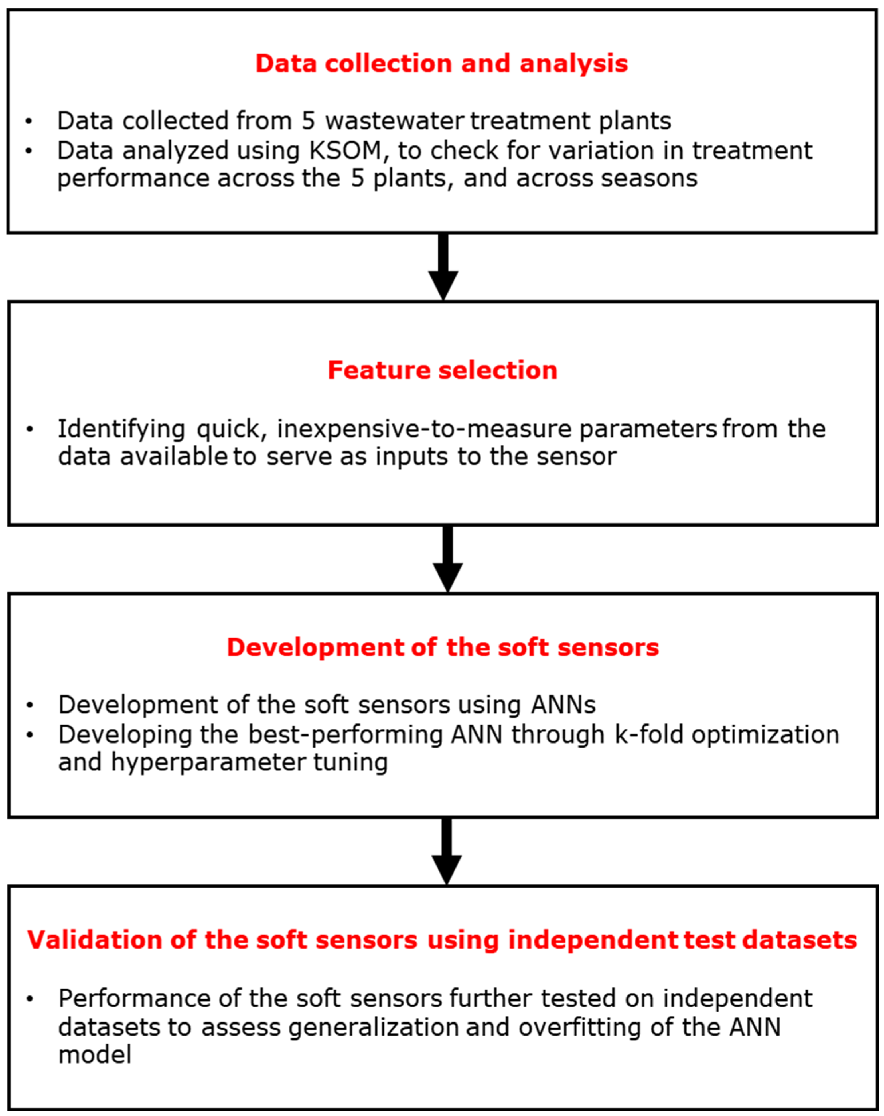
The development process for the soft sensors analyzing TSS, BOD, COD, TN, and TP is outlined in the following sections. A summary of these steps is provided in Figure 1.

2.1. Data Collection

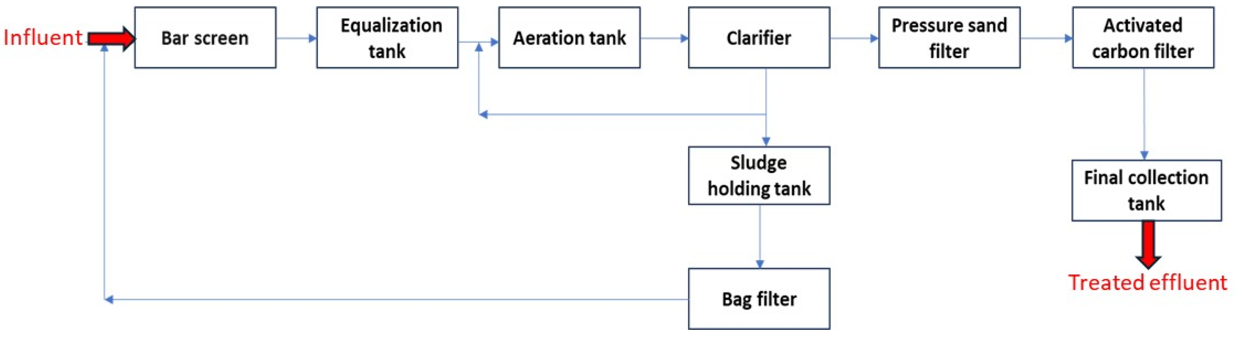
The data used to develop soft sensors for determining effluent organic matter and nutrient parameters was sourced from five modular wastewater treatment plants serving various residential complexes in Bangalore. The five plants treat wastewater generated from a total of 23 residential towers. The flow diagram of the treatment plants is shown in Figure 2. All the plants use the same extended aeration technology with the same treatment steps, only differing in their capacities (

Table 1. Details of the 5 modular wastewater treatment plants.

Plant Identifier	Capacity (Million L per Day)	Number of Residential Towers Served	Effluent Parameters Measured
1	620	6	pH, TSS, BOD, COD, total nitrogen, ammoniacal nitrogen, turbidity, total residual chlorine, total phosphorus, oil and grease, fecal coliform, E. coli.
2	500	5
3	380	4
4	500	4
5	500	4

). The treated effluent quality data were collected for a 3-year period, spanning 2019 to 2023. The datasets with incomplete entries were removed. From these, 156 complete datasets having the log of turbidity, TSS, BOD, and COD were used for the development of the soft sensor for TSS, BOD, and COD measurement. A total of 185 datasets had the requisite entries of turbidity, TN, and TP, and thus these datasets were used for the development of the TN and TP soft sensor.

2.2. Feature Selection

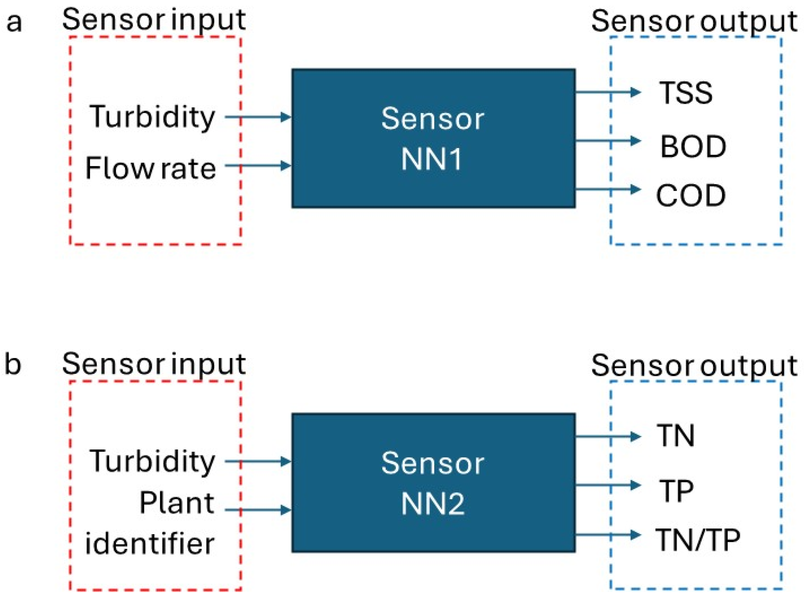
Feature selection is a critical step in neural network modeling as it directly influences the model’s performance and accuracy. By carefully choosing relevant input features, the predictive power of the model can be enhanced while reducing computational complexity and preventing overfitting. The aim of this work is to develop soft sensors to predict time-consuming and expensive-to-measure effluent quality parameters, using data from quick and inexpensive-to-measure parameters. Accordingly, from among the effluent quality parameters, pH and turbidity were identified as the quick, inexpensive, and easy-to-measure parameters. But as the pH showed barely discernable variation throughout the dataset, it was excluded from the input features. Consequently, turbidity was selected as the primary input feature. For the soft sensor model (named “NN1”) for measuring TSS, BOD, and COD, the capacity of the plant was also considered as an input (Figure 3a). Meanwhile for the soft sensor (named “NN2”) for TN and TP measurement, an identifier (1, 2, 3, 4, or 5) representing the specific plant was included as an input to the neural network (Figure 3b). The “NN” in the soft sensor model names stands for “neural networks”, as the models are based on artificial neural networks. The range of values of the effluent quality data for the chosen input (turbidity) and output parameters (COD, BOD, TSS, TN, and TP) is given in

Table 2. Effluent quality data.

Effluent Quality Parameter	Range (Minimum–Maximum)	Average
Turbidity (NTU)	0.1–2	0.71 ± 0.5
Total suspended solids (mg/L)	1–18.1	5.67 ± 2.9
Biochemical oxygen demand (mg/L)	2–9	5.25 ± 1.88
Chemical oxygen demand (mg/L)	7–48	27.51 ± 10.78
Total nitrogen (mg/L)	2.8–25.4	8.96 ± 4.16
Total phosphorous (mg/L)	0.2–4.5	1.49 ± 1.09

.

2.3. Data Analysis

As mentioned in the previous section, the data for developing the soft sensors were sourced from five modular wastewater treatment plants that treat wastewater generated by several residential complexes. Since the plants receive wastewater from households, the influent is expected to exhibit similar ranges of water quality parameters. Additionally, because all the plants follow the exact same sequence of treatment processes, it is anticipated that the effluent water quality parameters across all plants will also fall within a similar range. In order to confirm this, Kohonen self-organizing maps (KSOM) was used to identify if there were any clustering patterns in the effluent quality parameters associated with specific plants. KSOM is a widely recognized unsupervised neural network model for data clustering and visualization. In a typical map generated from a KSOM analysis, the depth of the colors between nodes signifies the degree of similarity or dissimilarity between datapoints. Lighter colors like yellow indicate high similarity, whereas darker colors such as red and black indicate decreasing levels of similarity. The KSOM toolbox in MATLAB 2019 was utilized for carrying out analysis on the data from the five treatment plants. If the KSOM indicated that there was no significant clustering of the data across the plants, it would support the conjecture that as the plants receive similar influent, and are based on the exact same treatment processes, they are performing identically even though their individual capacities are different. In that case, the data from all the plants could be grouped together and only one soft sensor model would be developed to serve all the plants.

2.4. Development of the Soft Sensor Models Using Artificial Neural Networks (ANNs)

Artificial neural networks were chosen to develop the soft sensors. ANNs are powerful tools in machine learning, known for their ability to handle complex, nonlinear relationships between inputs and outputs. ANNs are inspired by the working of the human brain, and a neural network functions similarly to how the human brain learns. The ANN begins by receiving input data through the input layer, which serves as the initial point of data acquisition. These data are then processed through the hidden layers, where mathematical operations such as weighted sums and activation functions are applied. These hidden layers introduce nonlinearity, allowing for the network to recognize and model complex patterns within the data. Upon completion of this processing, the data reach the output layer, which produces the final result or prediction. During the training phase, the network refines its predictions by continuously adjusting its weights to minimize the difference between its predicted outcomes and the actual target values. Each neuron within the network applies a transfer function, incorporating weights and biases to compute its output. As part of this learning process, the network updates these weights based on the input data and the expected output, gradually improving its accuracy over time.

The training algorithm, the number of hidden layers, number of neurons, and the activation (transfer) function used for developing the ANN model are key factors, referred to as hyperparameters, that significantly influence the performance of the model. The model performance is optimized by identifying the best configuration of the hyperparameters. This process significantly impacts the overall behavior and efficacy of the neural network. To begin, the first hyperparameter that was explored was the appropriate training algorithm to be used for developing the model. MATLAB (2019) software was used for the development of the model. As the software had 17 training algorithms in its repertoire, all 17 were explored (

Table 3. Training algorithms explored for hyperparameter tuning.

Function in the MATLAB (2019) Software	Training Algorithm Called by the Function
Trainlm	Levenberg–Marquardt back propagation
Trainscg	Scaled conjugate gradient back propagation
Trainbfg	BFGS Quasi Newton back propagation
Traincgb	Conjugate gradient back propagation with Powell–Beale restarts
Traincgf	Conjugate gradient back propagation with Fletcher–Reeves updates
Traincgp	Conjugate gradient back propagation with Polak–Ribiere updates
Traingd	Gradient descent back propagation
Traingda	Gradient descent with adaptive learning back propagation
Traingdm	Gradient descent with momentum
Traingdx	Gradient descent with momentum and adaptive linear back propagation
Trainoss	One step secant back propagation
Trainrp	RPROP back propagation
Trainb	Batch training with and bias learning rules
Trainc	Cyclical order weight/bias training
Trainr	Random order weight/bias training
Trains	Sequential order weight/bias training
Trainbr	Bayesian regularization back propagation

). The best-performing amongst the 17 was then chosen for further hyperparameter tuning.

Next, the number of neurons, transfer functions, and the number of hidden layers in the chosen training algorithm was varied to arrive at the best combination of hyperparameters in terms of performance. The number of neurons was varied from 1 to 20, and the number of hidden layers was varied from 1 to 2. For each neuron number and hidden layer combination, K-fold optimization was carried out. K-fold optimization is a cross-validation technique used to evaluate and optimize the performance of machine learning models. In k-fold cross-validation, the dataset is divided into k equally sized subsets, or “folds”. The model is trained on k − 1 folds and tested on the remaining fold. This process is repeated k times, with each fold serving as the test set once. The final performance metric is the average result across all folds, providing a more reliable assessment of model accuracy and generalization. In this study, k was set at 5, i.e., the total dataset was divided into 5 subsets (folds). Hence, for each fold, one fold was used for validation and the remaining 4 folds were used for training. Thus, for each fold, 4/5ths, i.e., 80%, of the data are used for training, and the remaining 1/5th, i.e., 20%, is used for validation.

The performance of the model was evaluated in terms of the coefficient of determination (R²), mean square error (MSE), mean absolute error (MAE), and the correlation (R) between the measured values and the values predicted by the ANN model. The performance plots of the model during the training and testing phase were also used to evaluate and compare the performance of the models. The best-performing combination of the number of neurons and hidden layers for the algorithm was chosen for the soft sensor.

Finally, to further validate the model’s performance, it was tested on a dataset that was not part of the data used for model development. The TSS, BOD, and COD soft sensor was tested against 47 such independent test datasets. The TN and TP soft sensor was tested against 25 such independent test datasets. Evaluating the model’s performance on this independent test set provides insights into its generalization ability and helps identify any potential overfitting.

3. Results and Discussion

3.1. Data Analysis

A KSOM was run on the data from the five treatment plants to check if there was any clustering observed amongst them. The absence of clustering would indicate that all the five plants perform similarly. The results of the KSOM are shown in Figure 4. From the maps, it can be seen that the data from the five plants were highly similar, with most nodes appearing yellow, indicating high similarity between the data from the five plants, and showing no significant plant-wise clustering. A few neurons in darker shades suggested minor differences, likely due to variations in operations or influent characteristics. The number of dissimilar datapoints were very few when compared with those that were similar, indicated by the predominance of light shades in the map. Consequently, it was concluded that the functioning of the five wastewater treatment plants can be considered identical, and a single neural network model could be used to effectively predict effluent quality parameters for all five wastewater treatment plants.

3.2. Development of the Soft Sensors Using ANN Models

Towards the development of the soft sensors, two distinct artificial neural network (ANN) models were crafted using MATLAB 2019 version, each tailored to predict specific effluent parameters from wastewater treatment plants. As the KSOM data analysis confirmed no significant clustering of the data from the five plants, the data from all the five plants were combined for the development of the soft sensor. The first senor model, NN1, for forecasting TSS, BOD, and COD, uses turbidity and plant capacity as input features. For NN1, a dataset of 156 datapoints was utilized for model development and validation, partitioned into 109 for the development of the model, and the remaining 47 sets for independent validation of the model. For the soft sensor NN2, designed to predict TN and TP, inputs comprised turbidity and an identifier. With 185 datapoints, 160 were used for training and the rest 25 datapoints were kept aside for independent validation of the sensor.

The first step towards the hyperparameter tuning was the selection of the training algorithm. For this, 17 training algorithms were explored (Table 3), and the performance of each in estimating the effluent quality parameters was evaluated. The results are presented in

Table 4. Comparison of the performance of various training algorithms for the soft sensor NN1 for TSS, BOD, and COD measurement (all algorithms employ 10 neurons and 1 hidden layer).

Training Algorithm	Training		Validation		Testing
	R	MSE	R	MSE	R	MSE
trainscg	0.8826	31.2682	0.9065	24.666	0.8859	35.78715
trainbr	0.889	30.439	NaN	NaN	0.957	10.43
trainlm	0.9412	14.0728	0.8664	55.725	0.8564	40.79
trainbfg	0.90343	27.6076	0.88193	24.4082	0.90284	26.9163
traincgb	0.86937	35.7047	0.89838	31.8362	0.81586	39.7849
traincgf	0.89727	29.0001	0.93227	16.5367	0.8507	35.836
traincgp	0.90641	26.4839	0.94634	15.7871	0.83628	39.816
traingd	−0.45076	22245.8	−0.63042	2093.8	−0.33954	2372.6
traingda	0.88353	32.8055	0.9314	15.1696	0.81869	55.4461
traingdm	0.33546	716.9368	0.39072	660.5115	0.11932	1023.7
traingdx	0.85705	41.7644	0.85195	35.8506	0.87197	34.2592
trainoss	0.91067	23.7069	0.8932	37.6923	0.90336	24.7799
trainrp	0.93435	18.8057	0.90591	24.7501	0.69293	64.5596
trainb	0.65549	95.1472	0.83936	66.6888	0.77943	66.102
trainc	0.10036	1.54 × 10127	−0.074539	1.39 × 10127	0.12553	1.37 × 10127
trainr	0.83943	45.8934	0.84707	36.9548	0.82245	49.3153
trains	0.91635	23.2929	NaN	NaN	0.87881	28.5717

and

Table 5. Comparison of the performance of various training algorithms for the soft sensor NN2 for TN and TP measurement (all algorithms employ 10 neurons and 1 hidden layer).

Training Algorithm	Training		Validation		Testing
	R	MSE	R	MSE	R	MSE
trainscg	0.8364	10.8772	0.5752	31.5953	0.7404	17.3069
trainbr	0.94	4.8	NaN	NaN	0.9047	6.83
trainlm	0.88651	8.303	0.76652	15.5428	0.89816	6.7624
trainbfg	0.6178	27.3695	0.6352	26.9588	0.5614	32.4081
traincgb	0.73296	17.7763	0.77101	14.4345	0.7175	18.4653
traincgf	0.79866	13.1069	0.73896	19.4733	0.71183	20.3635
traincgp	0.81	12.225	0.659	24.5668	0.665	21.3927
traingd	0.2835	385.4809	0.32931	374.4605	0.45894	366.6973
traingda	0.72489	18.1822	0.79099	12.8561	0.754	19.0128
traingdm	0.52458	126.2644	0.5808	137.002	0.61599	104.278
traingdx	0.79927	14.1637	0.60589	24.5994	0.62732	23.6649
trainoss	0.74185	17.5842	0.8012	10.7865	0.7689	16.7542
trainrp	0.74193	18.23402	0.71175	14.893	0.7121	18.4471
trainb	0.43228	56.0376	0.52339	46.7036	0.34588	71.4434
trainc	0.83	13.3231	0.789	19.2984	0.80322	22.4227
trainr	0.77559	17.6851	0.6191	31.5	0.64	27.0636
trains	0.80191	13.107	NaN	NaN	0.84421	12.8455

. From the results, it is seen that for both the soft sensors, the training algorithm trainbr emerged as the best performing one, exhibiting superior performance across essential metrics of correlation coefficient (R), mean squared error (MSE), and effectiveness depicted in performance plots and error histograms, across the training, validation, and testing datasets.

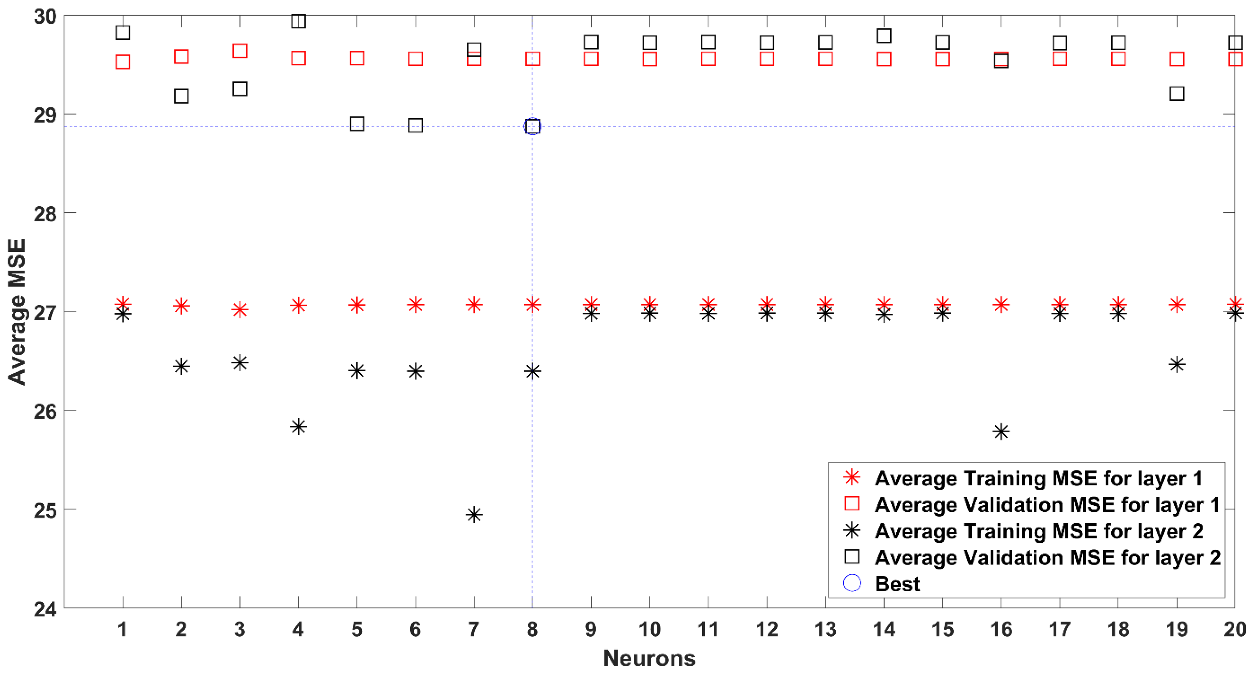
Having found the best training algorithm, the next step in the hyperparameter tuning was further refinement of its performance by exploring the effect of changing the number of neurons from 1 to 20, and the number of hidden layers from 1 to 2, and picking the best-performing combination. Each of these combinations of neurons and number of hidden layers was subjected to K-fold optimization. The resulting performance metrics are presented in Figure 5 and Figure 6.

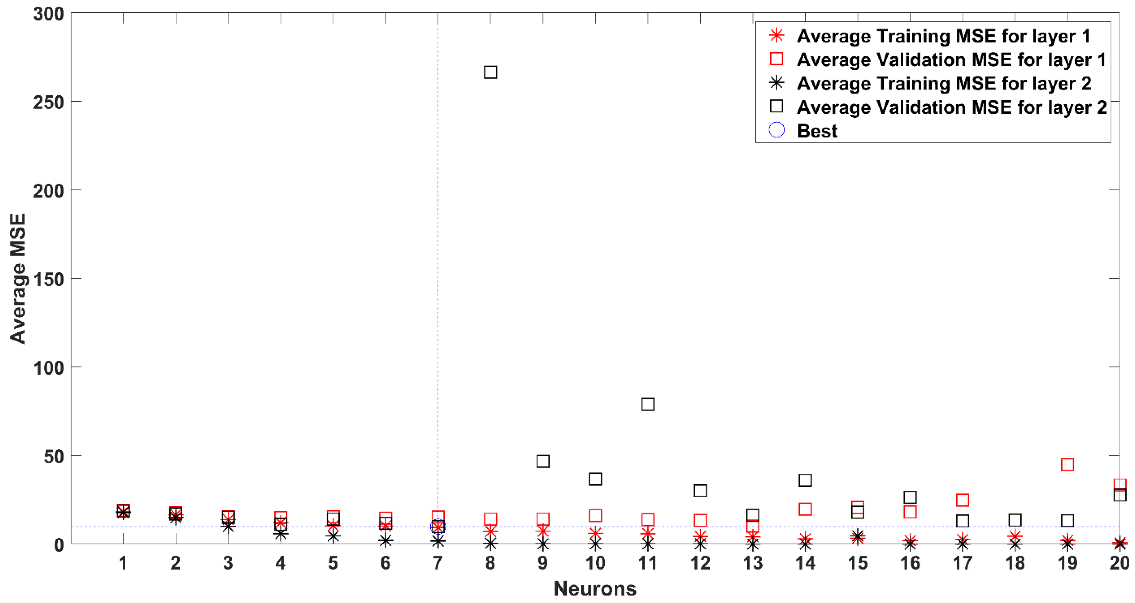
The figures plot the average MSE resulting from the k-fold optimization for each combination of neurons and hidden layers. During each k-fold optimization, the dataset is split into a training dataset and a validation dataset. The network is trained on the training dataset and validated on the validation dataset. The MSE of both the sets is plotted in Figure 5 and Figure 6. The combination of the number of neurons and hidden layers that gave the least MSE on the validation dataset is taken as the best performing combination and adopted for the soft sensor. From Figure 5, it can be seen that for the NN1 soft sensor, the combination of eight neurons and two hidden layers gave the least MSE and hence the best performance. For the NN2 soft sensor, it can be seen from Figure 6 that the combination of seven neurons and two hidden layers gave the best performance.

To summarize: The soft sensor NN1, developed for the measurement of TSS, BOD, and COD, is a neural network trained using the Bayesian regularization algorithm. It comprises two hidden layers with eight neurons, employing the “tansig” transfer function in the hidden layers and “purelin” in the output layer. Similarly, the soft sensor NN2, designed for the measurement of TN and TP, is also based on the Bayesian regularization algorithm. It features two hidden layers with seven neurons, utilizing the “tansig” transfer function for the hidden layers and “purelin” for the output layer.

The performance metrics of the developed sensors is presented in

Table 6. Performance of the soft sensor predictions on training dataset.

Parameter	R	R2	MSE	95% Confidence Interval of the MSE	MAE	95% Confidence Interval of the MAE
TSS	0.837	0.699	2.04	1.771–2.309	1.083	0.907–1.259
BOD	0.658	0.428	1.905	1.645–2.166	1.066	0.900–1.231
COD	0.694	0.477	69.09	67.53–70.65	6.039	4.962–7.117
TN	0.859	0.736	5.356	4.997–5.715	1.289	0.990–1.588
TP	0.84	0.702	0.392	0.295–0.489	0.454	0.386–0.521

. The metrics used were the correlation coefficient (R), the coefficient of determination (R²), mean squared error (MSE), and mean absolute error (MAE) of the actual (measured) values versus the soft sensor-predicted values. Further, the 95% confidence interval for the MSE and MAE is also presented. TSS and TP exhibit strong predictive performance, with R values of 0.837 and 0.84, respectively. Their R² values (0.699 and 0.702) suggest that around 70% of the variance in the data is explained by the model. The low MSE and MAE values, along with narrow 95% confidence intervals, further confirm model reliability for these parameters. TN also shows strong predictive capacity, with the highest R (0.859) and R² (0.736) among all parameters. Although its MSE and MAE are higher than those of TSS and TP, the tight confidence intervals suggest consistent performance. COD and BOD have a moderate predictive capability, having the lowest R and R² of the parameters. However, the narrow confidence intervals indicate stability in prediction errors.

3.3. Further Testing of the Accuracy of the Sensors on Independent Test Datasets

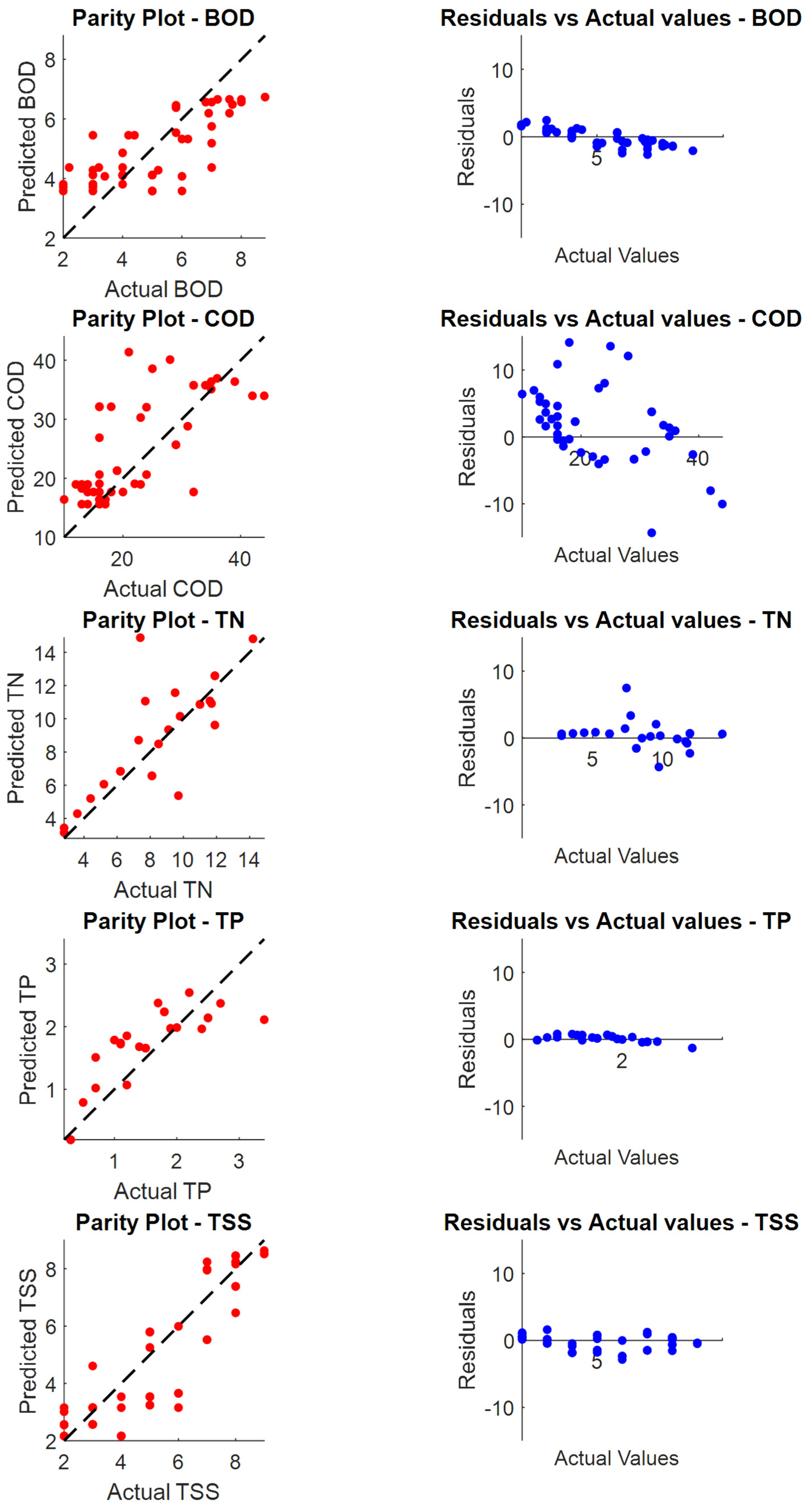
To further test the accuracy of the developed models, an independent test dataset that was not used for training was employed to verify the model’s generalization ability. The performance of the soft sensor NN1 for measuring effluent BOD, COD, and TSS was tested against 45 independent datasets. The soft sensor NN2 for measuring effluent TN and TP levels was tested against 25 independent datasets. The results are presented in Figure 7 and Figure 8, and

Table 7. Performance of the soft sensor predictions on the independent dataset.

Parameter	R	R2	MSE	95% Confidence Interval of the MSE	MAE	95% Confidence Interval of the MAE
TSS	0.878	0.718	1.34	1.022–1.659	0.93	0.731–1.13
BOD	0.761	0.546	1.575	1.215–1.935	1.08	0.895–1.265
COD	0.695	0.316	51.845	49.91–53.78	5.214	3.779–6.649
TN	0.795	0.541	4.31	3.496–5.125	1.311	0.667–1.955
TP	0.794	0.596	0.242	0.054–0.429	0.395	0.279–0.512

. The parity plots of the soft sensor-predicted data versus the measured data, alongside plots of the residuals versus measured data, of sensor NN1, are shown in Figure 7. Figure 8 shows similar results for the soft sensor NN2.

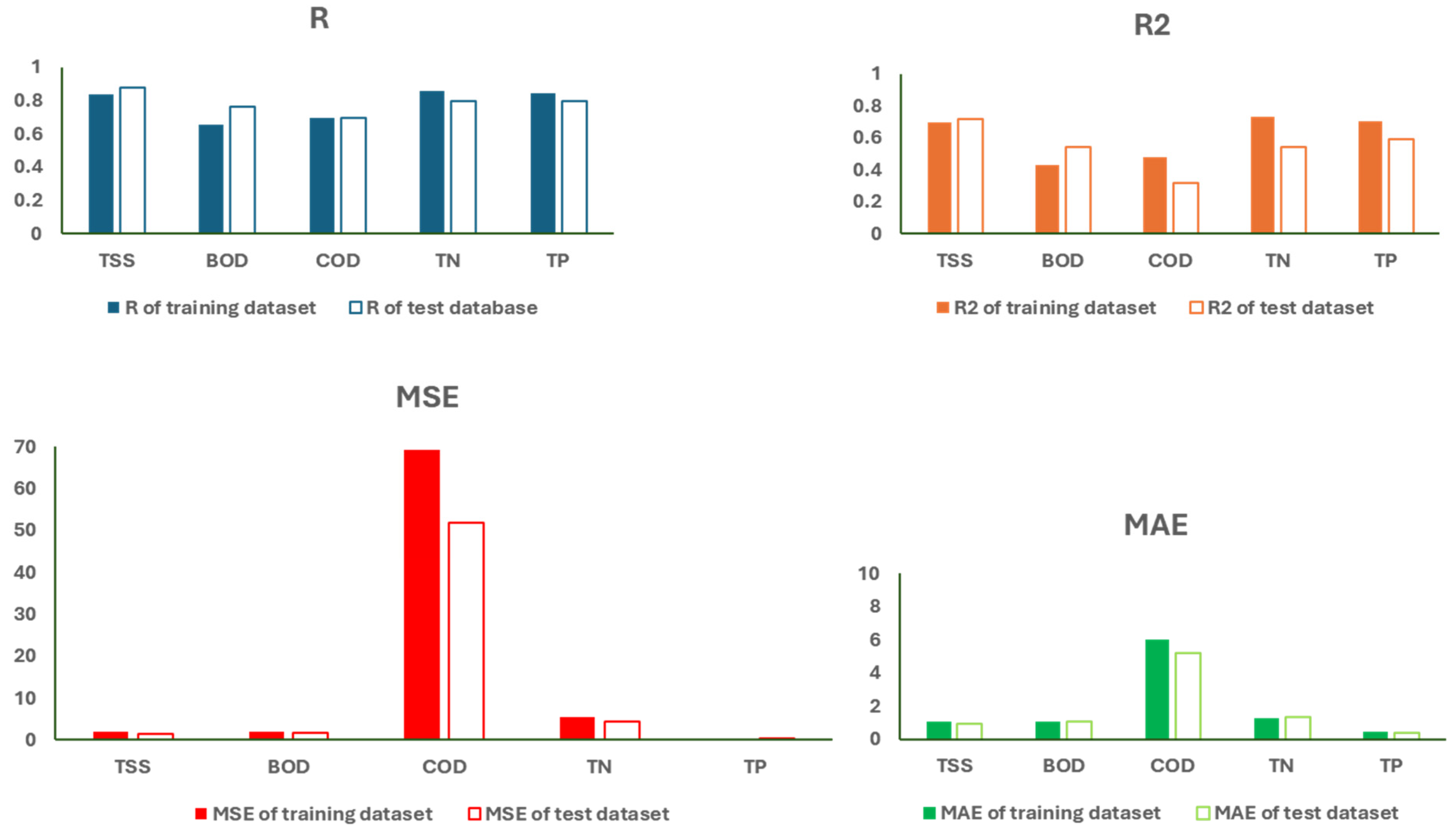
The performance metrics on the validation dataset, in terms of R, R², MSE, and MAE along with their 95% confidence intervals, is presented in Table 7. A plot comparing the R, R², MSE, and MAE of the sensors on the training dataset versus the validation dataset is presented in Figure 9. Ideally, for a well-generalized network, it is expected that the R and R² for any new dataset should be the same or higher than on the training dataset. Conversely, the MSE and MAE of the new dataset should be same or lower than the training dataset.

It can be seen from Figure 9 that the R of the validation dataset is higher than the training dataset for TSS, BOD, and COD, while it is marginally lower for TN and TP. The R² of the validation dataset is higher for TSS and BOD, and lower for the rest of the parameters. However, crucially, the MSE and MAE are lower than the training dataset for all the parameters. Further inference on the performance can be drawn by comparing the 95% confidence interval of the MSE and MAE of the training dataset (Table 6) with that of the independent validation dataset (Table 7).

The analysis of the training and test data for TSS shows that there is no overlap between the training and test MSE confidence intervals, indicating a significant positive difference in MSE between the training and test data. However, the training and test MAE confidence intervals overlap, meaning there is no significant difference in MAE between the two datasets. For BOD, there is overlap between the training and test MSE confidence intervals, suggesting no significant difference in MSE between the datasets, and similarly, the MAE confidence intervals overlap, showing no significant difference in MAE. In the case of TN, there is overlap in both the training and test MSE and MAE confidence intervals, indicating no significant differences in either MSE or MAE. Finally, for TP, the confidence intervals for both MSE and MAE overlap between the training and test data, suggesting no significant differences in either metric. For COD, the training and test MSE confidence intervals do not overlap, indicating a significant negative difference in MSE between the training and test data, but the MAE confidence intervals overlap, meaning no significant difference in MAE. In summary, significant differences in MSE are found only for TSS and COD, while for BOD, TN, and TP, no significant differences are observed in either MSE or MAE. Thus, overall, it can be concluded that the ANN models the sensors are based on have good generalization, are neither over- or underfitted, and are able to handle new independent data without significant difference in the performance of the sensors.

4. Summary and Conclusions

This paper addresses the problem of inadequate monitoring of wastewater treatment plants, especially in developing nations, due to cost constraints and limited resources. This can lead to the discharge of inadequately treated wastewater into the environment. To address this issue, this study explores the use of artificial intelligence (AI)-based soft sensors and virtual instruments for quick and inexpensive monitoring of effluent quality. This approach simplifies the monitoring process, making it more efficient for operators to ensure compliance with environmental standards without the need for complex and time-consuming laboratory analyses. Towards this, two soft sensors have been developed using artificial neural networks (ANNs) to predict effluent quality parameters, based on data from five modular wastewater treatment plants in Bangalore, India. The first sensor predicts total suspended solids (TSS), biochemical oxygen demand (BOD), and chemical oxygen demand (COD), while the second predicts total nitrogen (TN) and total phosphorus (TP). Both models use turbidity, an easily measurable parameter, as the input.

The methodology used to develop the soft sensors included data analysis using Kohonen self-organizing maps (KSOM), and the development of ANN models and their extensive testing and validation. The KSOM analysis showed no significant clustering of data based on plant identifiers, supporting the conjecture that all five plants were performing similarly, despite their varying capacities. As a result, the data from all the plants were grouped together, and a unified soft sensor model was developed. Artificial neural networks were chosen for this study due to their ability to model complex, nonlinear relationships between input features and output parameters. To begin the model development process, various hyperparameters were explored, including the training algorithm, number of neurons in the hidden layers, activation functions, and the number of hidden layers. MATLAB 2019 was used for the development of the model, and 17 different training algorithms were tested to determine which one produced the best performance. Bayesian regularization was identified to be the best-performing training algorithm for both the sensor models. Next, the number of neurons and hidden layers were varied, and K-fold cross-validation was employed to optimize the model. The performance of the soft sensor models was evaluated using various metrics, including R² (coefficient of determination), MSE (mean squared error), MAE (mean absolute error), and R (correlation coefficient) between the actual and predicted values. The 95% confidence intervals of the MSE and MAE were also determined. The soft sensor developed for the measurement of TSS, BOD, and COD comprises two hidden layers with eight neurons. The soft sensor designed for the measurement of TN and TP features two hidden layers with seven neurons. Both the ANN models utilize the “tansig” transfer function for the hidden layers and “purelin” for the output layer.

To further validate the model’s performance and generalization ability, the soft sensor models were tested against independent datasets that were not part of the data used for model development. The results confirmed the models’ generalization ability and absence of overfitting, and the model’s robustness and its ability to accurately predict effluent quality on new data with similar performance as during the development phase.

This study demonstrates the potential of AI-based soft sensors for monitoring wastewater effluent quality in modular treatment plants. It provides a foundation for future research on the development and refinement of soft sensor models. Additionally, it presents an opportunity to explore their integration with other monitoring systems, enhancing their application across various wastewater treatment technologies, configurations, and target contaminants. The findings of this research contribute to the advancement of wastewater treatment technology and pave the way for more sustainable and effective wastewater management strategies.