Enhancing Pipeline Leakage Detection Through Multi-Algorithm Fusion with Machine Learning

Abstract

This paper proposes a pipeline leakage detection technology that integrates machine learning algorithms with Dempster–Shafer (DS) evidence theory. By implementing five machine learning algorithms, this study constructs pipeline pressure and flow signal characteristics through wavelet decomposition. The data were normalized and processed using principal component analysis to prepare the algorithm for training. A new method for constructing basic probability functions using a confusion matrix and a simple support function is proposed and compared with the traditional triangular fuzzy number method. The basic probability function of the identification sample is refined by calculating a comprehensive discount factor. Finally, the results from multiple algorithms are fused using DS evidence theory. Experimental results demonstrate that after combining multiple algorithms, the average accuracy improves by 0.1565%, and the precision of the triangular fuzzy number method is enhanced by 0.091%.

1. Introduction

As petroleum and gas pipelines age, their structural integrity deteriorates, which makes pipeline safety a critical concern. Given the flammable and explosive nature of oil and gas products, pipeline leakage incidents can have severe and often irreversible consequences for society. This highlights the importance of effective leakage detection as a fundamental component of pipeline safety management, ensuring the secure and reliable operation of pipeline systems.

Pipeline leakage detection technologies use various techniques to determine whether a leak has occurred by analyzing changes in key parameters. These methods include the negative pressure wave method [1,2], the acoustic method [3,4,5], optical fiber sensing [6], flow modeling [7,8], big data analytics, and machine learning algorithms [9].

Among these, machine learning (ML) algorithms [10,11] have emerged as a highly effective approach for classification and prediction tasks in big data environments. In leakage detection studies, the issue is usually presented as a binary classification task. Several ML algorithms have been widely applied in this domain, including support vector machine (SVM) [12,13,14], logistic regression (LR) [10,11,15], decision tree (Classification and Regression Tree, CART) [16,17], random forest (RF) [18,19,20,21], and backpropagation neural network (BPNN) [22,23,24,25,26]. These algorithms offer high accuracy, ease of implementation, and strong adaptability, making them widely adopted in leakage detection applications. Their continued development has significantly enhanced the precision and efficiency of pipeline leakage detection systems.

In pipeline leakage detection research, single-method approaches are often used to identify leaks, limiting the ability to leverage the advantages of various detection techniques. Moreover, while some systems integrate multiple detection methods, these methods typically operate independently and trigger alarms separately. This results in an excessive number of leakage alarms, creating challenges for operators in managing and verifying alerts. Therefore, there is an urgent need for a unified approach to evaluate leakage alarm information from multiple detection methods, which will enhance the reliability of alarms while reducing false or redundant notifications. In response to these challenges, this study proposes a multi-algorithm fusion framework based on ML and Dempster–Shafer evidence theory (DS) [27,28]. ML algorithms are employed to identify pipeline leakage status. A novel method for constructing basic probability assignment (BPA) functions based on a confusion matrix and a simple support function (SSF) is proposed and compared with the conventional triangular fuzzy number (TFN) method. Furthermore, a discount factor is computed based on the results of multiple algorithms to evaluate the reliability of each algorithm, and the BPA of each sample is adjusted accordingly. Finally, the refined probability assignments are processed using DS evidence fusion theory to generate a unified recognition result, enhancing the precision and reliability of leakage alarms. Therefore, the advantage of this method is that the constructed BPA can be dynamically modified according to the performance of the algorithm, allowing the DS evidence fusion theory to combine the advantages of various algorithms to produce a more reliable BPA and improve the accuracy of the algorithm.

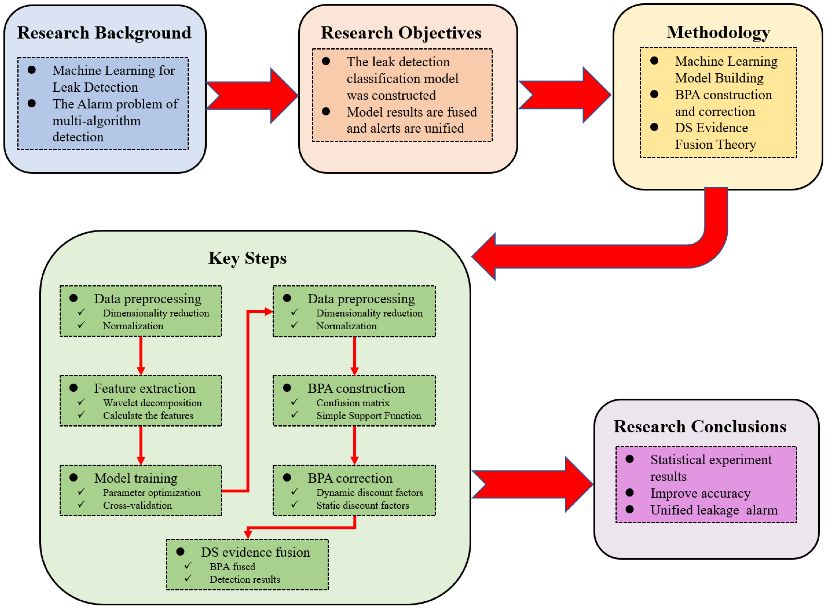
The arrangement of sections and the workflow of this paper are shown in Figure 1. Section 1 provides an overview of the causes of pipeline leakage incidents, their significance, classification, and the development of leakage detection technologies, with a focus on advancements driven by ML algorithms in recent years. Section 2 presents the theoretical foundations and computational processes of ML models. It outlines the calculation process of TFN, the determination of discount factors, and the application of DS evidence fusion theory in pipeline leakage detection systems. Section 3 presents and analyzes the target recognition results obtained using the methods outlined in Section 2. Section 4 presents the main conclusions of this study, summarizing the key innovations, findings, and contributions of the study while discussing future research directions and potential advancements in pipeline leakage detection.

2. Materials and Methods

2.1. Machine Learning Algorithms

2.1.1. Support Vector Machines

The core idea of SVM is to maximize the margin of classification. The basic model is a linear classifier with the maximum margin in the feature space. Using a kernel function transforms it into a nonlinear classifier. It has several advantages, including high efficiency for high dimensional data, strong generalization ability, a kernel function that can adapt to complex nonlinear decision boundaries, and robustness.

The regression function of a nonlinear SVM is expressed as:

$$f\left(x\right)=sign\left(\sum _{i=1}^N{\alpha }_i^{*}{y}_{i}K\left(x,x_i\right)+b^{*}\right)$$

(1)

where ${\alpha }_i^{*}{y}_i$ represents the weight vector, $K\left(x,x_i\right)$ is the kernel function, and $b^{*}$ denotes the bias term, b* = 0.5640. A dataset $T=\left\{\left(x_1,y_1\right),\left(x_1,y_1\right),\dots ,\left(x_N,y_N\right)\right\}$ is considered, where $x_i\in R^n,y_i\in \left\{+1,-1\right\},i=1,2,\dots N$.

An appropriate kernel function $K\left(x,z\right)$ and a penalty factor $C>0$ are selected, and initial C = 1. Then, the problem is formulated as a convex quadratic programming optimization, as follows:

$$\underset{\alpha }{\min }{\displaystyle \frac{1}{2}}\sum _{i=1}^N\sum _{j=1}^N{\alpha }_i{\alpha }_j{y}_i{y}_{j}K\left(x_i,x_j\right)-\sum _{i=1}^N{\alpha }_i$$

(2)

$$s.t.\hspace{0.33em}\hspace{0.33em}\hspace{0.33em}\hspace{0.33em}\sum _{i=1}^N{\alpha }_i{y}_i=0, 0 \le {\alpha }_i \le C,\hspace{1em}i=1,2,\dots ,N$$

(3)

Solving this optimization problem yields the optimal solution ${\alpha }^{*}={\left({\alpha }_1^{*},{\alpha }_2^{*},\dots ,{\alpha }_N^{*}\right)}^T$, ${\alpha }^{*}={\left(-200.0,-200.0,\dots ,\mathrm{0.3877,0.3683}\right)}^T$.

From this, ${\alpha }^{*}$ is selected, with ${\alpha }_j^{*}$ satisfying the condition $0<{\alpha }_j^{*}<C$, with the bias term computed as follows:

$$b^{*}=y_j-\sum _{i=1}^N{\alpha }_i^{*}{y}_{i}K\left(x_i,x_j\right)$$

(4)

For small datasets, the Lagrange operator is introduced to transform the problem into a least squares optimization, ultimately yielding the following function:

$$f\left(x\right)=sign\left(\sum _{i=1}^N{\alpha }_i^{*}{y}_{i}K\left(x,x_i\right)+b^{*}\right)$$

(5)

where $K\left(x,z\right)$ is a kernel function, which is calculated as follows:

$$K\left(x,z\right)=exp\left(-{‖x-z‖}^2/2{\sigma }^2\right)$$

(6)

where x and z represent the sample points, ${‖x-z‖}^2$ is the square of the Euclidean distance between two points, and σ is used to control the super parameter of the width of the Gaussian function, with a value of 1.8708.

2.1.2. Logistic Regression

When logistic regression (LR) is used for classification, the primary objective is to minimize the cost function, which quantifies the difference between the predicted results and the actual values. The optimization process yields the optimal model parameters. The advantages include strong interpretability of the model and output, high computational efficiency, suitability for big data, strong ability to model linear relationships, regularization to avoid overfitting, and good robustness to noise and missing data.

The sigmoid function, which maps any input to a probability value between 0 and 1, is depicted in Figure 2.

$$g\left(z\right)={\displaystyle \frac{1}{1+e^{-z}}}$$

(7)

$$z={\theta }^{T}x$$

(8)

where x is the normalized input vector, θ are the model coefficients to be solved, $\theta ={\left(-0.0038,0.0572,0.0741,0.0511,0.0651,0.0957,0.0741\right)}^T$, and z is a linear combination of the input features. The hypothesis function for logistic regression is formulated as follows:

$$h_{\theta }\left(x\right)=g\left({\theta }^{T}x\right)={\displaystyle \frac{1}{1+e^{-{\theta }^{T}x}}}$$

(9)

The cost function is expressed as follows:

$$\begin{array}{l}J\left(\theta \right)=-{\displaystyle \frac{1}{m}}\left[{\displaystyle \sum _{i=1}^m}{y}^{\left(i\right)}{\mathit{log}h}_{\theta }\left(x^{\left(i\right)}\right)+\left(1-y^{\left(i\right)}\right)\left(1-{\mathit{log}h}_{\theta }\left(x^{\left(i\right)}\right)\right)\right]\\ \hspace{0.17em}\hspace{0.17em}\hspace{0.17em}\hspace{0.17em}\hspace{0.17em}\hspace{0.17em}\hspace{0.17em}\hspace{0.17em}\hspace{0.17em}\hspace{0.17em}\hspace{0.17em}\hspace{0.17em}\hspace{0.17em}\hspace{0.17em}\hspace{0.17em}\hspace{0.17em}\hspace{0.17em}\hspace{0.17em}\hspace{0.17em}+{\displaystyle \frac{\lambda }{2m}}{\displaystyle \sum _{j=1}^n}{\theta }_j^2\end{array}$$

(10)

where m is the number of training samples, $y^{\left(i\right)}$ represents the true label in the data set, $h_{\theta }\left(x^{\left(i\right)}\right)$ is the model predicted value, and ${\displaystyle \frac{\lambda }{2m}}{\sum }_{j=1}^n{\theta }_j^2$ is the regularization term to mitigate overfitting. To minimize the cost function, the gradient descent update rule is applied as follows:

$${\theta }_j:={\theta }_j-\alpha {\displaystyle \frac{1}{m}}\sum _{i=1}^m\left(\left(h_{\theta }\left(x^{\left(i\right)}\right)-y^{\left(i\right)}\right)·x_j^{\left(i\right)}+{\displaystyle \frac{\lambda }{m}}{\theta }_j\right)$$

(11)

where α is the learning rate, initial α = 0.1, λ is the regularization penalty factor, and initial λ = 1.

2.1.3. Decision Tree and Random Forest

Decision trees (Classification and Regression Tree, CART) and random forests (RF) are both tree-based machine learning algorithms. CART starts at the root node, evaluates feature attributes, selects an output branch, and ultimately reaches a leaf node that contains the final decision result. In contrast, random forest is an ensemble learning method that combines multiple decision trees to enhance performance. The final classification result is calculated by averaging the results of multiple decision trees. The advantages of decision trees include high interpretability, low data preprocessing requirements, handling of nonlinear relationships and complex boundaries, high computational efficiency, fast training speed, and in-sensitivity to noise and outliers. The advantages of RF include high prediction accuracy and generalization ability, processing of high-dimensional data and complex nonlinear relationships, evaluation of global feature importance, and parallel calculation.

During the construction of each decision tree, the node-splitting process is guided by a measure of feature purity. Each feature split results in a reduction in information gain. In classification trees, the Gini coefficient is commonly used to evaluate the purity of a node. It is calculated as follows:

$$gini\left(T\right)=1-\sum _{i=1}^k{p}_i^2$$

(12)

where T represents the training set, k is the number of categories, k = 2, and p_i represents the probability that a sample in T belongs to category i. The Gini coefficient is calculated for sub-nodes T₁ and T₂ as follows:

$$gini\left(T_1,T_2\right)={\displaystyle \frac{\left|T_1\right|}{\left|T\right|}}gini\left(T_1\right)+{\displaystyle \frac{\left|T_2\right|}{\left|T\right|}}gini\left(T_2\right)$$

(13)

2.1.4. Back Propagation Neural Networks

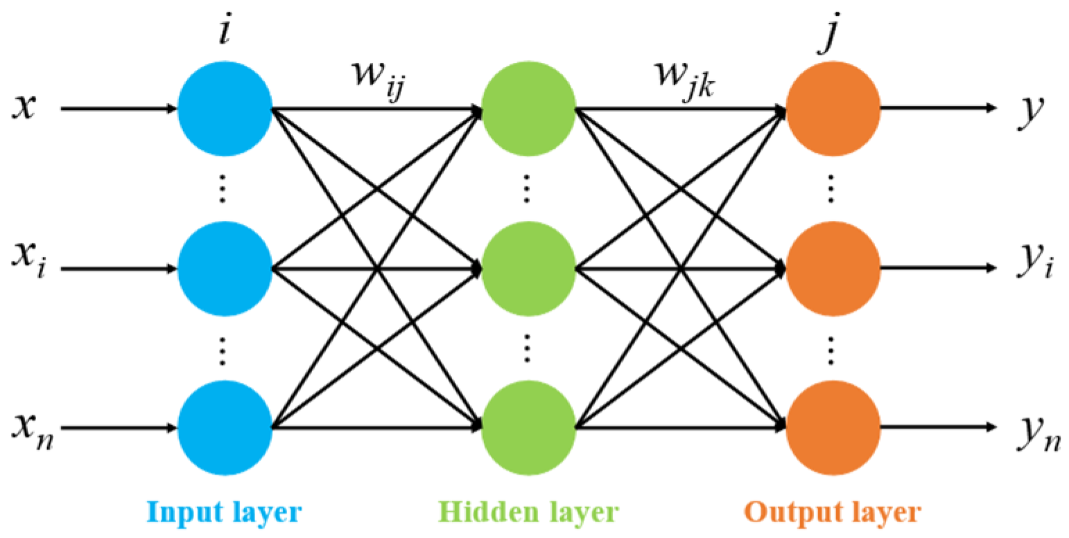
Back Propagation Neural Networks (BPNN) are a type of feedforward network that utilizes error backpropagation for optimization. The overall structure and functioning of BPNN are illustrated in Figure 3. Its self-learning process involves both information forward propagation and error backpropagation. During forward propagation, the data are passed from the input layer. If the actual output of the output layer does not meet the expectation, error backpropagation is performed, and the weights of each node layer are adjusted according to the error. Because of the ability to adjust for reverse errors, determining the relationship between input and output is easy. Its advantages include strong nonlinear modeling ability, self-learning feature representation, parallel computing ability, and good scalability, which can suppress overfitting and improve generalization performance, as well as suitability for high-dimensional and complex data. The self-learning process of BPNN consists of two main stages: forward propagation of information and backpropagation of errors [26].

Let each sample be denoted as $(\overrightarrow{x},\overrightarrow{t})$, where $\overrightarrow{x}$ represensts the input features and $\overrightarrow{t}$ denotes the target values.

The process begins by using the sample feature $\overrightarrow{x}$ to calculate the ai for each node in the hidden layer and the output y_i for the output layer. Then, we calculate error ${\delta }_i$ for the output layer nodes as follows:

$${\delta }_i=y_i(1-y_i)(t_i-y_i)$$

(14)

In addition, error ${\delta }_i$ for the hidden layer nodes is calculated as follows:

$${\delta }_i=a_i(1-a_i)\sum _{k\in outputs}{w}_{ki}{\delta }_k$$

(15)

where w_ki represents the weight between node i and its next layer node k, and ${\delta }_k$ denotes the error associated with the output node.

Finally, the weights are updated as follows:

$$w_{ji}\leftarrow w_{ji}+\eta {\delta }_j{x}_{ji}$$

(16)

where w_ji is the weight from node i to node j, η is the learning rate, and η = 0.001. In the initial state, where i = 7, the error $\delta =(0.2626,-0.1277,-0.0976, 0.34242913, 0.1739,-0.1277, 0.028)$, and the weight matrix w_ji is as shown in

Table 1. The weight calculation result of BPNN when i = 7.

Weight wji
0.81640	0.35886	−0.15987	−0.8469	0.90479	0.62690	0.14812
−0.55377	−0.30087	−0.02488	0.16883	−0.40796	0.23653	−0.40548
0.37193	−0.07894	−0.32382	−0.45112	−0.27903	−0.29779	−0.031705
−0.06405	−0.17081	−0.04535	0.75670	−0.08225	0.33138	−0.67731
0.0118	−0.14734	−0.17138	−0.19283	−0.56859	−0.59765	0.56937
−0.36591	−0.39003	0.21496	0.46997	0.317602	−0.83157	0.39756
0.01968	0.63045	−0.00333	0.57800	−0.62835	0.40632	−0.62823

:

2.2. Triangular Fuzzy Number

For target recognition, the minimum, maximum, and average values of a specific indicator from the sample data can be obtained [28]. A TFN can be constructed based on these values. TFN is especially important in DS evidence fusion theory because it can deal with multi-source heterogeneous data better than other methods in the field of multi-sensor fusion. At the same time, it is an important method to construct BPA functions based on the membership degree of TFN. Its advantage is that the mathematical characteristics of TFN make the operation rules clear, the computational complexity is low, the calculation is efficient and simple to implement, the modeling is intuitive, and the interpretability is strong.

As shown in Figure 4, two TFNs $\stackrel{`}{A}$ and $\stackrel{`}{B}$ are defined as:

$$\stackrel{`}{A}=\left(a_1,a_2,a_3;w_1\right),0<w_1\le 1$$

(17)

$$\stackrel{`}{B}=\left({\beta }_1,{\beta }_2,{\beta }_3;w_2\right),0<w_2\le 1$$

(18)

The membership function ${\mu }_{\stackrel{`}{A}}$ for TFN $\stackrel{`}{A}$ is constructed as follows:

$${\mu }_{\stackrel{`}{A}}=\left\{\begin{array}{c}0,x\le a\\ {\displaystyle \frac{x-a}{b-a}}\times w,a<x\le b\\ {\displaystyle \frac{c-x}{c-b}}\times w,b<x<c\\ 0,x\ge c\end{array}\right.$$

(19)

where a, b, and c are the minimum, maximum, and mean, respectively, w is the membership function value when x = b, initial w = 1.0, $\stackrel{`}{A}=\left(\mathrm{0,0.422,1};1.0\right)$, and $\stackrel{`}{B}=\left(\mathrm{0.028,0.464,0.998};1.0\right)$.

Assume the recognition framework for target recognition is $\Theta =\{{\theta }_1,{\theta }_2,\dots ,{\theta }_n\}$. For an observed target $o\left(o\in {\theta }_i,i=1,\dots ,n\right)$, the classifiers S₁, …, S_k, …, S_K correspond to the K indicators of the recognition category. For each category θ_i, the recognition result vector of each classifier S_K for each training sample ${\mathsf{\chi }}_{im}$ is defined as $t_k\left({\mathsf{\chi }}_{im}\right)={\left[t_k^{{\mathsf{\chi }}_{1m}}\left({\mathsf{\theta }}_1\right),\cdots ,t_k^{{\mathsf{\chi }}_{im}}\left({\mathsf{\theta }}_i\right),\cdots ,t_k^{{\mathsf{\chi }}_{nm}}\left({\mathsf{\theta }}_n\right)\right]}^T$.

Where $t_k\left({\mathsf{\chi }}_{im}\right)$ represents the measure that classifier S_K assigns to the sample ${\mathsf{\chi }}_{im}$ belonging to the category θ_i. Assuming θ_i has M_K samples, for indicator k, the following calculations are performed as follows:

$$a_k\left({\theta }_i\right)=min\left(t_k^{{\chi }_{i1}}\left({\theta }_i\right),t_k^{{\chi }_{i2}}\left({\theta }_i\right),\cdots ,t_k^{{\chi }_{i{M}_i}}\left({\theta }_i\right)\right)$$

(20)

$$b_k\left({\theta }_i\right)={\displaystyle \frac{1}{M}}\sum _{m=1}^{M_k}{t}_k^{{\chi }_{im}}\left({\theta }_i\right)$$

(21)

$$c_k\left({\theta }_i\right)=max\left(t_k^{{\chi }_{i1}}\left({\theta }_i\right),t_k^{{\chi }_{i2}}\left({\theta }_i\right),\cdots ,t_k^{{\chi }_{i{M}_i}}\left({\theta }_i\right)\right)$$

(22)

The strategy for generating BPA using the TFN representation model can be described as follows:

(1) Case 1: If m = 0, this indicates that the measurement value for indicator k is outside the minimum and maximum range for all categories. The measurement value does not intersect with any TFN representation model, i.e., m(Θ) = 1 or m($\varnothing$) = 1.

(2) Case 2: If m = 1, the measurement value V intersects with the TFN representation of a single-element proposition. In this case, the ordinate of the intersection point ${\mu }_{H_i}^k$ represents the support of the measurement value V for the single-element proposition.

(3) Case 3: If m > 1, the measurement value V intersects with the TFN representation of multiple propositions. The maximum ordinate of the intersection point is considered the support of the measurement value V for the single-element proposition.

(4) Generating BPA: After obtaining the support for each proposition, the BPA can be generated using the following two methods:

The maximum membership value is subtracted from 1 and is assigned to the whole set Θ. This represents the part of the information considered to be completely unknown, i.e., ${Sup}_{\Theta }^k=1-max{\mu }_{H_i}^k,\left(i=1,2,\cdots ,m\right)$, and initial ${\mu }_{H_0}^1$ = 0.

The support values ${\mu }_{H_j}^k$ of each proposition obtained from the above strategy to calculate the BPA for each proposition are normalized as follows:

$$\left\{\begin{array}{c}m\left(H_j\right)={\displaystyle \frac{Su{p}_{H_j}^k}{{\sum }_{i=1}^{p}Su{p}_{H_i}^k+Su{p}_{\Theta }^k}},H_j\in 2^{\Theta },H_j\ne \Theta \\ m\left(\Theta \right)={\displaystyle \frac{Su{p}_{\Theta }^k}{{\sum }_{i=1}^{p}Su{p}_{H_i}^k+Su{p}_{\Theta }^k}}\end{array}\right.$$

(23)

Then, the calculation formula of W₁ is used to normalize the new support ${Sup}_{H_j}^k$ and obtain the BPA for each proposition.

2.3. Machine Learning Algorithms in Pipeline Leak Detection

2.3.1. Training Machine Learning Algorithms

• Dataset

This study utilizes Pipeline Studio V4.0.1.0 software to simulate pipeline leakage detection, generating pipeline operation data as input data for ML algorithms. A total of 150 simulated leakage datasets were generated, with each simulation providing both normal operation and leakage data, resulting in a total of 300 datasets. The numerical simulation considers variations in starting pressure, pipeline diameter, and leakage. The simulation parameters are summarized in

Table 2. Parameter selection range for leakage data.

Simulation Parameter	Value Range
Starting pressure	1, 2, 3, 4, 5 MPa
Ending pressure	0.5 MPa
Pipe diameter	0.05, 0.1, 0.2, 0.3, 0.4, 0.5 m
Leakage rate	5%, 10%, 15%, 20%, 25%

.

The schematic diagram of the simulated pipeline model is shown in Figure 5.

2.

Features

For the pipeline leakage detection problem, this study directly selects pressure and flow as the primary features. In many pipeline leakage detection methods, common features include energy and envelope spectrum entropy. In this paper, wavelet packet analysis is employed to construct energy features. The process involves performing wavelet packet analysis on the data using MATLAB R2016a V9.0 software, followed by calculating the energy of the decomposed signal [14].

3.

Data dimensionality reduction

To reduce the dimensionality of the data, the principal component analysis (PCA) algorithm is applied.

4.

Data preprocessing

Data preprocessing refers to the transformation of raw data into a format suitable for model training, aiming to enhance the quality of the input data. In this study, both flow and pressure data are normalized to map them to the [0, 1] range. The normalization process is defined as follows:

$$x={\displaystyle \frac{x-x_{min}}{x_{max}-x_{min}}}$$

(24)

5.

Algorithm training

The grid search method is used to train the model, and 5-fold cross-validation is employed to evaluate the model’s performance. This process aims to determine the optimal parameter combination to enhance the algorithm’s efficiency. According to the experience of a large number of experiments, the selection range for the initial values of the model parameters is presented in

Table 3. Selection range of model parameters.

Method	Parameters	Values
SVM	Kernel	linear, rbf, poly, sigmoid
	C	0.01–100
LR	Solver	lbfgs, liblinear, newton-cg
	C	0.01–100
	Penalty	l1, l2
RF	Max_depth	1–5
	n_estimators	1–3
CART	Max_depth	1–5
	Criterion	gini, entropy, log_loss
BPNN	Nnits	10–300
	Epochs	100
	Batch_size	100

.

6.

Result evaluation

To evaluate the classification ability of the model, a confusion matrix and overall precision are utilized.

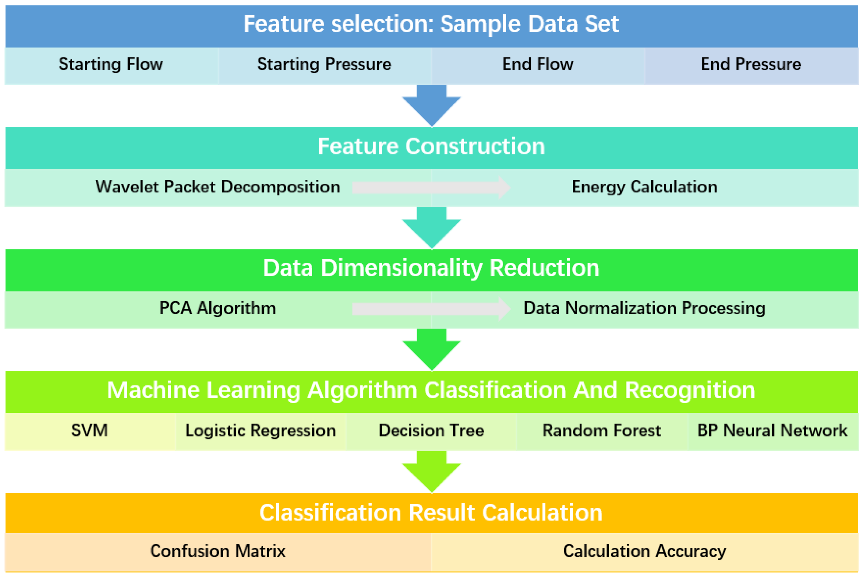
The target classifiers for pipeline leakage detection based on each algorithm were implemented in Python V3.8.5, with the Sklearn library handling all classifier functionalities. The calculation process is depicted in Figure 6. The training process of the algorithm includes obtaining the data set through numerical simulation, constructing the features of the data, and calculating the energy features after the data are decomposed by a wavelet packet. The PCA algorithm is used to reduce the dimensions of the data, which are then normalized. Finally, the machine learning model is trained, and the target is recognized.

2.3.2. Construction of the Basic Probability Assignment (BPA) Function

In the multi-information fusion model proposed in this paper, four pieces of evidence (starting flow, ending flow, starting pressure, and ending pressure) are used, with five algorithm classifiers trained on these respective datasets. The recognition framework is Θ = (leakage, no leakage), where event A represents leakage and event B represents no leakage. The algorithm constructs the BPA, which consists of the following steps:

(1) Method 1: BPA calculation using Xu’s method: For a given classifier, the classification result is expressed by the confusion matrix C_k, which is then normalized. This method was previously proposed in [27].

$$C_k=\left[\begin{array}{ccccc}{r}_{11}^{\left(k\right)}& r_{12}^{\left(k\right)}& \cdots & r_{1M}^{\left(k\right)}& r_{1M+1}^{\left(k\right)}\\ r_{21}^{\left(k\right)}& r_{22}^{\left(k\right)}& \cdots & r_{2M}^{\left(k\right)}& r_{2M+1}^{\left(k\right)}\\ \cdots & \cdots & \cdots & \cdots & \cdots \\ r_{M1}^{\left(k\right)}& r_{M2}^{\left(k\right)}& \cdots & r_{MM}^{\left(k\right)}& r_{MM+1}^{\left(k\right)}\end{array}\right]$$

(25)

where $r_{ij}^{\left(k\right)}={\displaystyle \frac{n_{ij}^{\left(k\right)}}{N_i^{\left(k\right)}}}$, with $n_{ij}^{\left(k\right)}$ representing the sample size for a specific category, and $N_i^{\left(k\right)}(i\in (1,2,\cdots ,M\left)\right)$ is the total sample size for the i-th category, defined as $N_i^{\left(k\right)}={\sum }_{j=1}^{M+1}{n}_{ij}^{\left(k\right)}$.

Specifically, for the classifier treating output category ω_j, the BPA is calculated as follows:

$$p\left({\omega }_j\right)={\displaystyle \frac{{\sum }_{i=1}^M{r}_{ii}}{M}}$$

(26)

$$p\left(\Omega \right)=1-{\displaystyle \frac{{\sum }_{i=1}^M{r}_{ii}}{M}}$$

(27)

(2) Method 2: BPA calculation using SSF (simple support function). The BPA calculation process based on a SSF was proposed by Xie [28]. The BPA is given as follows:

$$p\left({\omega }_i\right)=p\left({\displaystyle \frac{{\omega }_i}{{\omega }_j}}\right)={\displaystyle \frac{r_{ij}}{{\sum }_{j=1}^M{r}_j}}$$

(28)

$$m\left({\omega }_i\right)=p\left({\omega }_i\right)$$

(29)

$$m\left(\Omega \right)=1-p\left({\omega }_i\right)$$

(30)

where $i=\{1,2,\dots ,M\}$.

This paper uses both of the above strategies to calculate the BPA and compares them to explore a more accurate BPA construction method.

2.4. Calculation of Comprehensive Discount Factor

2.4.1. Static Discount Factors α and β

There are two types of static discount factors, α and β, each calculated differently and exhibiting distinct capabilities. This study compares both methods.

$${\alpha }_i=D_{BBA}(BB{A}_i,BB{A}_0),(i=1,2,\cdots ,N)$$

(31)

where α_i represents the static discount factor of the i-th sample, N is the total number of samples, BPA_i represents the BPA of the _i-th sample, BPA₀ denotes the BPA of the actual output for the sample, and D_BBA represents the Jousselme distance.

The calculation for the reliability of the classifier is expressed as follows:

$$p\left({\omega }_i\right)=p\left({\displaystyle \frac{{\omega }_i}{{\omega }_i}}\right)={\displaystyle \frac{r_{ii}}{{\sum }_{i=1}^M{r}_i}}$$

(32)

The reliability actor is given as follows:

$$R_n=p\left({\displaystyle \frac{{\omega }_i}{{\omega }_i}}\right)={\displaystyle \frac{r_{ii}}{{\sum }_{i=1}^M{r}_i}}$$

(33)

The static discount factor is calculated as follows:

$${\beta }_n=1-R_n=1-{\displaystyle \frac{r_{ii}}{{\sum }_{i=1}^M{r}_i}}$$

(34)

2.4.2. Dynamic Discount Factor γ

To evaluate the mutual support reliability between classifiers, the dynamic discount factor γ is introduced. Its calculation process is as follows:

$$\left\{\begin{array}{c}\rho \left(m_i,m_j\right)={\displaystyle \frac{<m_i,m_j>}{\left|m_i\right|\left|m_j\right|}}\\ \mathit{sup}(S_k)={\displaystyle \sum _{j=1,j \ne k}^K}\rho \left(m_k,m_j\right)\\ \begin{array}{c}{R}^{\prime }(s_k)={\displaystyle \frac{\mathit{sup}(S_k)}{{\sum }_{k=1}^k\mathit{sup}(S_k)}}\\ R(s_k)={\displaystyle \frac{R^{\prime }(s_k)}{\underset{k=1,\cdots ,K}{max}\{R^{\prime }(s_k)\}}}\in [0,1]\\ {\gamma }_k=1-R(s_k),(k=1,2,\cdots ,K)\end{array}\end{array}\right.$$

(35)

where m_i and m_j are the BPA calculated by the i-th and j-th classifiers of the training sample O_i, respectively. ρ represents the correlation coefficient, $\mathit{sup}(S_k)$ is the support degree, $R^{\prime }\left(s_k\right)$ is the relative support degree, and $R\left(s_k\right)$ is the absolute reliability.

2.4.3. Comprehensive Discount Factor

By combining both static discount factors, a comprehensive factor for the k-th classifier is computed using the weighted average, with initial $p_k$ = 0.5.

$$\begin{gathered} {\alpha }_k^{\prime }=p_k{\alpha }_k+\left(1-p_k\right){\gamma }_k,p_k\in \left[0,1\right],\left(k=1,2,\cdots K\right) \\ {\alpha }_k^{\prime }=p_k{\beta }_k+(1-p_k){\gamma }_k,p_k\in [0,1],(k=1,2,\cdots K) \end{gathered}$$

(36)

2.5. Dempster–Shafer Evidence Theory

In Dempster–Shafer (DS) evidence theory [29], the identification framework Θ is defined as a set of n mutually exclusive elements, $\Theta =\{{\theta }_1,{\theta }_2,\dots ,{\theta }_n\}$, where θ_i (1 ≤ i ≤ n) represents a single subset of Θ that contains all objects. The power set $2^{\Theta }$ represents the set of all subsets of Θ.

2.5.1. DS Evidence Fusion Rules

Two credibility functions, Bel₁ and Bel₂ [30], are defined in the same framework Θ, with corresponding assignments m₁ and m₂. The focal elements of evidence are $A_1,A_2\cdots A_m$ and $B_1,B_2\cdots B_n$. The basic probability assignments for these focal elements are $m_1\left(A_1\right),m_1\left(A_2\right),\cdots m_1\left(A_m\right)$ and $m_2\left(B_1\right),m_2\left(B_2\right),\cdots ,m_2\left(B_n\right)$). Given that ${\sum }_{A_i\cap B_j=\mathsf{\Phi }}{m}_1\left(A_i\right)m_2\left(B_j\right)<1$, the basic credibility distribution of the two credibility functions, Bel₁ and Bel₂, is computed by the following function $m:2^{\mathsf{\Theta }}\to [0,1]$, expressed as follows:

$$m\left(X\right)=\left\{\begin{array}{c}{\displaystyle \frac{{\sum }_{A_i\cap B_j=X}{m}_1\left(A_i\right)m_2\left(B_j\right)}{1-{\sum }_{A_i\cap B_j=\Phi }{m}_1\left(A_i\right)m_2\left(B_j\right)}}\\ 0,X=\phi \end{array}\right.,\forall A\subseteq \Theta ,X\ne \phi$$

(37)

where φ denotes the empty set, and $m\left(\phi \right)=0$, considering m₁, m₂,…, m_n.

2.5.2. Application of Multi-Algorithm Fusion in Leak Detection

Discount operations based on the Shafer discount rule are used for identifying target $O_i(i=1,2,\cdots ,N)$. After obtaining the comprehensive discount factor ${\alpha }_k^{\prime }$ from the confusion matrix of classifier S_k, the comprehensive reliability factor $R_k^{\prime }=1-{\alpha }_k^{\prime }$ is calculated. Guided by this approach, the Basic Probability Assignment (BPA) output by classifier S_k for the identification target O_i is adjusted according to its corresponding comprehensive discount factor.

Once the discount factor is determined by evaluating the classifiers’ reliability, it is applied to the output evidence of the local classifier, thereby enabling the discount operation on the respective BPA [31]. This paper employs the classical Shafer discount rule for this purpose. The rule is defined as follows:

$$m\left(A\right)=\left\{\begin{array}{c}(1-{\alpha }^{\prime })m_k\left(A\right),A\subset \Omega \\ \left(1-{\alpha }^{\prime }\right)m_k\left(A\right)+{\alpha }^{\prime },\mathrm{A}=\Omega \end{array}\right.$$

(38)

where initial ${\alpha }^{\prime }$ = 0.5. By applying the Shafer discount rule, the modified BPA is obtained as $BPA=\left\{p\right({\omega }_1),p({\omega }_2),p(\Omega \left)\right\}$. Finally, after applying a betting transformation, the final $BPA=\left\{p\right({\omega }_1^{\prime }),p({\omega }_2^{\prime }\left)\right\}$ is derived and used as the input for the Dempster–Shafer (DS) decision algorithm.

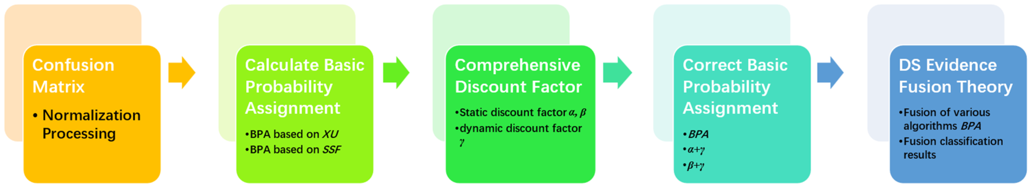
The model progression procedure is depicted in Figure 7. The calculation process of the model includes the following steps: first, the confusion matrix is obtained from the classification results of the machine learning algorithm, which is then normalized, and the BPA function is calculated using Methods 1 and 2. Then, the static, dynamic, and comprehensive discount factors (α, β, γ) are calculated, and the BPA is corrected using various combinations of discount factors. Finally, the BPA is combined with DS evidence to produce a unified classification result.

3. Results

3.1. PCA Calculation Results

The 4-dimensional pressure flow data at both ends of the pipeline is decomposed using wavelet transformation. Each signal is further decomposed into 8-dimensional data, which enables the calculation of the signal’s energy. After performing wavelet analysis on the dataset to construct features, a 32-dimensional dataset is obtained. However, for the selected ML algorithm, the dimensionality of the data is too high, necessitating dimensionality reduction. This study utilizes the PCA algorithm for this purpose. The PCA calculation results are presented in Figure 8 and

Table 4. Principal component F_k values for PCA dimensionality reduction.

Principal Component Fk	Explained Variance Ratio (%)
F1	54.46
F2	73.60
F3	85.64
F4	93.62
F5	96.51
F6	98.15
F7	99.35

.

3.2. Classification Results of ML Algorithms

3.2.1. Classification Results

The classification and recognition results of each algorithm are displayed in Figure 9 and

Table 5. Comparison of classification accuracy across various algorithms.

Method	Classification Accuracy (%)
SVM	0.807
LR	0.743
RF	0.873
CART	0.753
BPNN	0.834

.

3.2.2. Results of Discount Factor

The average dynamic, static, and comprehensive discount factor results are calculated according to the BPA constructed using Method 1, which are shown in

Table 6. Calculation results of different discount factors in Method 1.

Method	Average Static Discount Factor α	Average Static Discount Factor β	Average Dynamic Discount Factor γ
SVM	0.538	0.161	0.071
LR	0.675	0.297	0.064
RF	0.185	0.090	0.242
CART	0.658	0.265	0.068
BPNN	0.458	0.113	0.085

and

Table 7. Calculation results of comprehensive discount factors using Method 1.

Method	Comprehensive Discount Factor α + γ	Comprehensive Discount Factor β + γ
SVM	0.350	0.116
LR	0.486	0.181
RF	0.138	0.166
CART	0.462	0.167
BPNN	0.286	0.099

, while the results of Method 2 are shown in

Table 8. Calculation results of different discount factors in Method 2.

Method	Average Static Discount Factor α	Average Static Discount Factor β	Average Dynamic Discount Factor γ
SVM	0.424	0.161	0.086
LR	0.562	0.297	0.060
RF	0.187	0.091	0.237
CART	0.544	0.265	0.069
BPNN	0.350	0.113	0.095

and

Table 9. Calculation results of comprehensive discount factors in Method 2.

Method	Comprehensive Discount Factor α + γ	Comprehensive Discount Factor β + γ
SVM	0.293	0.124
LR	0.430	0.179
RF	0.139	0.164
CART	0.405	0.167
BPNN	0.232	0.104

.

3.2.3. Calculation Results of DS Evidence Fusion

The classification accuracy of multi-algorithm fusion based on DS evidence theory using different methods is shown in

Table 10. Comparison of DS fusion results for different methods.

BPA Construction Method		Classification Accuracy (%)
Method 1	Xu + α + γ + DS	0.983
	Xu + β + γ + DS	0.947
Method 2	SSF + α + γ + DS	0.977
	SSF + β + γ + DS	0.923

. The comparison of the classification accuracy of the TFN method using DS fusion is presented in

Table 11. Classification accuracy of TFN.

BPA Construction Method	Dataset	Classification Accuracy (%)
		DS Before Fusion	DS After Fusion
TFN	Starting flow	0.814	0.903
	Starting pressure	0.785	0.873
	Ending flow	0.823	0.903
	Ending pressure	0.772	0.880

.

4. Discussion

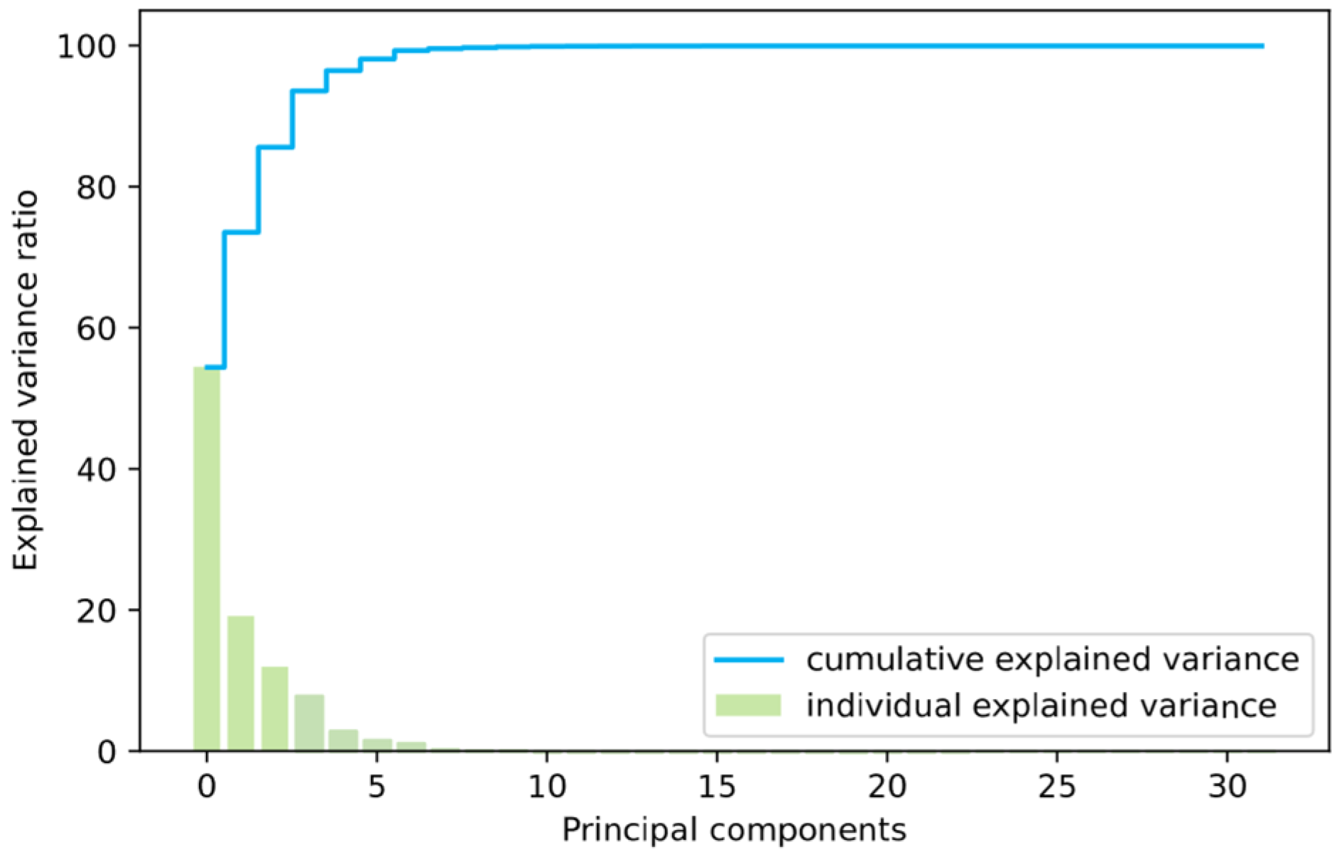
As shown in Figure 8 and Table 4, the cumulative variance of the first seven principal components exceeds 99%, which is sufficient to capture the main characteristics of the dataset. Consequently, the original dataset is reduced to a 7-dimensional form.

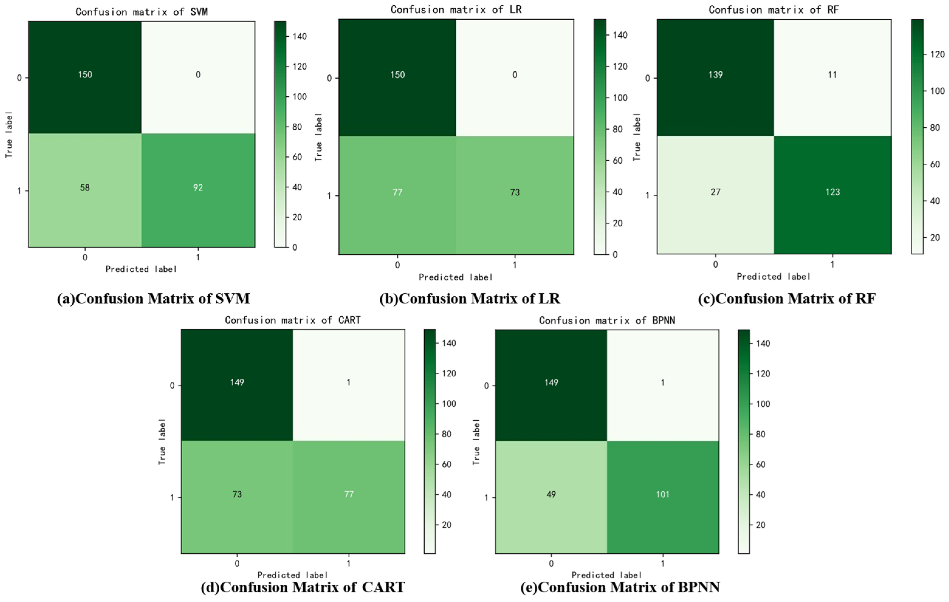
The classification and recognition results of each algorithm are displayed in Figure 9 and Table 5. The classification accuracies for each algorithm are as follows: SVM (0.807%), LR (0.743%), RF (0.873%), CART (0.753%), and BPNN (0.834%). The average accuracy across all algorithms is 0.802%. Among these, the RF algorithm achieves the highest accuracy due to its ensemble nature. The BPNN algorithm follows closely, as its neural network structure, with a large number of neurons, provides a more effective simulation of the data, yielding better classification performance.

Method 1 calculates the average discount factor based on Xu’s method, with the results for α, β, and γ presented in Table 6. It is evident that the LR and CART algorithms exhibit a larger discount for α and β, while the RF algorithm shows a higher discount for γ. The results of the comprehensive discount factor are presented in Table 7. It can be observed that the combination of α + γ yields a larger overall discount, whereas the combination of β + γ results in a smaller discount. Additionally, both combinations lead to greater discounts for the LR and CART algorithms. Furthermore, Method 2 calculates the average discount factor using the SSF method. The results for α, β, and γ are presented in Table 8. It is evident that the average static discount factors α and β exhibit a larger discount for the LR and CART algorithms, whereas the average dynamic discount factor γ indicates a higher discount for the RF algorithm. The calculation results of the comprehensive discount factor are shown in Table 9. It can be observed that the combination of α + γ yields a larger overall discount, while the combination of β + γ results in a smaller discount. Both combinations also lead to larger discounts for the LR and CART algorithms, a trend that is consistent with the results from Method 1.

The calculation results of the multi-algorithm fusion based on DS evidence theory for different methods are presented in Table 10. It is evident that the classification accuracy for the BPA method based on Xu’s study’s findings is 0.983% and 0.947%. For the BPA method using SSF, the classification accuracy is 0.977% and 0.923%. Additionally, the classification accuracy using the comprehensive factor α + γ is higher than that of β + γ, with increases of 0.006% and 0.024%, respectively. Overall, the classification accuracy achieved by the DS evidence fusion algorithm surpasses that of single ML algorithms.

In addition, the accuracy comparison for the TFN method is presented in Table 11. Before the DS evidence fusion, the classification accuracy is 0.814%, 0.785%, 0.823%, and 0.772%, with an average precision of 0.799%. After the DS evidence fusion, the classification accuracy improves to 0.903%, 0.873%, 0.903%, and 0.880%, with an average precision of 0.890%. The classification accuracy of the comprehensive factor-modified BPA method proposed in this paper is significantly higher than the traditional TFN-based BPA method. Moreover, the target recognition and BPA construction method using ML-based approaches outperform the traditional BPA construction method of TFN.

The multi-algorithm fusion method is effective because the DS evidence fusion theory can combine the detection results of each ML algorithm and calculate the comprehensive discount factor of the BPA of each algorithm for the sample, resulting in higher accuracy. Specifically, for samples with conflicting classification results in ML algorithms, considering the difference in recognition ability of each algorithm for different categories and the mutual support between algorithms, the correct classification results in the DS evidence fusion process are increased by the comprehensive discount factor to modify the BPA, and the classification accuracy of pipeline leak detection is improved. In addition, DS evidence fusion will provide a unified detection result, potentially reducing false and repeated alarms in the leak detection system.

On the other hand, the reliability of the performance indicators of the classification algorithm is tested, and the confidence interval of the accuracy quantifies the estimation uncertainty of the model accuracy.

Table 12. Comparison of 95% confidence intervals for the accuracy of various ML algorithms.

Method	Accuracy Confidence Intervals
SVM	[0.7600, 0.8500]
LR	[0.6933, 0.7933]
RF	[0.8500, 0.9201]
CART	[0.7000, 0.8033]
BPNN	[0.8000, 0.8800]

and Figure 10 show the calculation results for each algorithm’s accuracy and 95% confidence interval. The analysis of the confidence interval reveals that the interval range of each algorithm is large, and its credibility and accuracy are low.

The accuracy and confidence intervals calculated using the DS fusion method are shown in

Table 13. Comparison of DS fusion 95% confidence interval results for different methods.

BPA Construction Method		Accuracy Confidence Intervals
Method 1	Xu + α + γ + DS	[0.967, 0.993]
	Xu + β + γ + DS	[0.925, 0.954]
Method 2	SSF + α + γ + DS	[0.961, 0.988]
	SSF + β + γ + DS	[0.907, 0.941]

and Figure 11. The analysis of the confidence interval indicates that the interval range of the DS fusion method is smaller, and the calculation accuracy and reliability of the algorithm are greater.

The statistical test determines whether the difference in the performance of the classification algorithm is statistically significant. That is, it determines whether there is a significant difference in performance between two classifiers on the same dataset. The t-test was conducted with the following null hypothesis H₀: there is no significant difference between the two models. The significance level is α = 0.05. If the calculated p-value is less than α, the null hypothesis is rejected, indicating a significant difference in performance between the two models. Otherwise, the null hypothesis is accepted, and the model performance difference is insignificant. The significance levels of the machine learning algorithm and the algorithm fused in this paper were compared, and their p-values were calculated as shown in

Table 14. Comparison of p-values calculated by machine learning and fusion algorithms.

Model	Method 1		Method 2
	Xu + α + γ + DS	Xu + β + γ + DS	SSF + α + γ + DS	SSF + β + γ + DS
SVM	0.0000004929	0.0000161632	0.0000004142	0.0000020924
LR	0.0000000035	0.0000000065	0.0000000022	0.0000000019
RF	0.0000003435	0.0000197874	0.0000002348	0.0002462460
CART	0.0000000831	0.0000003110	0.0000001274	0.0000001688
BPNN	0.0000003524	0.0000030773	0.0000002068	0.0000246338

. We can see that all p-values < 0.05, indicating that the null hypothesis is rejected and that the differences between the algorithms are significant.

The fused methods were compared for significance levels, and p-values were calculated, as shown in

Table 15. The p-value comparison was calculated between the fusion methods.

Model		Method 1		Method 2
		Xu + α + γ + DS	Xu + β + γ + DS	Xu + α + γ + DS	Xu + β + γ + DS
Method 1	Xu + α + γ + DS	—	0.0000150190	0.2326774765	0.0000397548
	Xu + β + γ + DS	0.0000150190	—	0.0001031786	0.0460293027
Method 2	SSF + α + γ + DS	0.2326774765	0.0001031786	—	0.0000288065
	SSF + β + γ + DS	0.0000397548	0.0460293027	0.0000288065	—

. It can be seen that in Xu + α + γ + DS of Method 1 and SSF + α + γ + DS of Method 2, the calculated p-value is 0.23267 > 0.05; thus, the null hypothesis is accepted, and the difference between these two construction methods is not significant. The other p-values < 0.05 reject the null hypothesis and indicate a significant difference between the various algorithms.

The robustness of the method proposed in this paper can be addressed through data preprocessing, which uses standardization and normalization methods to process the data. During the feature selection, a single feature is avoided, and flow and pressure data are used for feature extraction. In the model selection and training, the regularization of LR, the dropout parameter in BPNN, and cross-validation in the model training process are used to prevent overfitting and improve the robustness of the method. In addition, the robustness of the method can be further improved by including sensor noise or random disturbance in the data, as well as actual pipeline leakage data, to enrich the dataset.

The limitation of this paper is that only the flow and pressure are considered in the data, and no actual pipeline leakage data are included. In order to apply the algorithm to the detection of actual leakage events, the data sample size should be larger. Only the leakage results from the ML algorithm were fused, but the detection results from the traditional physical model were not. In subsequent research, real leakage data and multi-source sensor data, such as sound, will be considered to build more waveform, time, and frequency domain features, and other BPA construction methods will be investigated for decision fusion and other methods for improvement. At the same time, heuristic optimization methods can be considered to optimize the hyperparameters of the model, while deep learning algorithms, such as the Long Short Term Memory network (LSTM), convolutional neural network (CNN), and other models, can be used for classification and recognition.

5. Conclusions

This paper proposes a multi-algorithm fusion method based on the ML and DS evidence fusion theory. Various machine learning models, such as SVM, LR, CART, RF, and BPNN algorithms, are used to identify pipeline leakage targets. The energy calculation method of wavelet packet analysis is used for feature construction, and the PCA algorithm is used to reduce the dimension of the data, and then the data are normalized. Two BPA construction methods based on Xu and SSF methods are proposed, as well as the comprehensive discount factor that includes both static discount factors (α, β) and dynamic discount factors (γ). A BPA correction scheme based on these comprehensive discount factors is proposed. To achieve uniform recognition results and improve alarm accuracy, this paper proposed a BPA fusion method based on DS evidence fusion. After fusing the two ML algorithms, the average accuracy is increased by 0.1565%, and the average accuracy is increased by 0.091% after fusing the TFN method.

Future research can focus on developing a unified evaluation framework that integrates both prior knowledge-based methods with data-driven analysis. Specifically, for alarm results generated by traditional techniques, such as pressure analysis and leak detection models, it would be valuable to explore how to develop a comprehensive and unified evaluation method that combines multiple algorithms. This approach could then be enhanced with emerging ML algorithms to achieve more cohesive analysis results, ultimately improving the precision and effectiveness of the system.