Dynamic Coupling Model of the Magnetic Separation Process Based on FEM, CFD, and DEM

Abstract

Magnetic separation is an important method in the processing process, and its essence is the targeted dispersion of the mineral processing slurry pulp in the magnetic field space. The slurry is a complex multiphase fluid system with continuous phase carrying a large number of discrete phase particles, in which the magnetic particles agglomerate, migrate, and disperse under the dominance of magnetic force. In this process, there is nonlinear and unstable dynamic coupling between the continuous phase (liquid) and the discrete phase (solid particles) and between the discrete phases. In this paper, a dynamic cyclic multi-dipole magnetic moment algorithm with a higher calculation accuracy is innovatively proposed to calculate the magnetic interaction force between particles. Moreover, the P-E magnetization model suitable for a two-dimensional uniform magnetic field is further improved and optimized to make it applicable to a three-dimensional gradient magnetic field. Finally, based on the coupling of the Finite Element Method (FEM), Computational Fluid Dynamics (CFD), and Discrete Element Method (DEM), a dynamic coupling model capable of accurately simulating the magnetic separation process is developed. This model can be used to study the separation behavior of particles under a multiphase flow and multi-force field and to explore the motion behavior of magnetic particles.

1. Introduction

Magnetic separation is an important physical ore dressing method that utilizes the magnetic differences among minerals to achieve the separation of ores in a non-uniform magnetic field [1]. The magnetic separation process is complex and usually involves the particle dynamics behavior under the action of a solid–liquid or solid–gas multiphase flow and multiple force fields, including the magnetic field, flow field, and gravitational field. Magnetic separation technology has a development history of hundreds of years. However, the magnetic separation process has always been difficult to observe at the microscopic level, especially the magnetic aggregation process formed after the magnetic particles are magnetized, as well as its generation, fracture, combination, and reconstruction.

Over the past more than ten years, the dynamic coupling method of multiphase flow and multi-physical fields based on FEM (Finite Element Method), CFD (Computational Fluid Dynamics), and DEM (Discrete Element Method) has developed rapidly. Most researchers have carried out the simulation of the magnetic separation process based on the coupling of multiphase flow and multi-physical fields and particle dynamics through Monte Carlo simulation, LB-DEM, N-S dynamics, and FEM-CFD-DEM coupling simulation methods, thus truly achieving the “visualization” of the magnetic separation process [2]. Murariu [3] combined DEM, CFD, and FEM and carried out secondary development to establish a coupling model, and for the first time the full-process simulation of the separation of minerals by a permanent magnet drum magnetic separator was achieved. Lindner et al. [4] for the first time used the coupling technology of CFD, FEM, and DEM to realize the simulation of particle capture by single wire and multiple wires in HGMS. Hu [5], based on the dynamic coupling model of FEM, CFD, and DEM, proposed the key technologies, simulation steps, and function evaluation, etc., that need to be solved in the full-process simulation of the magnetic separation by a permanent magnet drum magnetic separator. Wu et al. [6] used the coupling method of FEM, CFD, and DEM to study the movement law and influencing factors of magnetite particles in a three-product magnetic separation column. Based on the interaction of ideal dipoles, Pinto-Espinoz [7] established a theoretical mathematical model of the magnetic force between magnetic particles, that is, the classical Pinto-Espinoza magnetization model, which laid the foundation for the simulation research of ferromagnetic particles. Chen et al. [8] combined CFD and DPM coupling to simulate the particles in the fluidized state and proposed an improved P-E magnetization model.

The above-mentioned models have problems, which are mainly manifested in the fact that when calculating the magnetic interaction force between particles based on the magnetic dipole model, a large number of idealized conditions are set, resulting in a large difference in the calculation accuracy of the long-range force and the short-range force, or there is no real dynamic coupling among multiple force fields. This paper innovatively proposes a dynamic cyclic multi-dipole magnetic moment algorithm for calculating the magnetic interaction force between particles. Compared with the traditional dipole model and its improved models, it has a higher calculation accuracy and a wider application range. Moreover, the P-E magnetization model adapted to the two-dimensional uniform magnetic field is further improved and optimized to make it suitable for the three-dimensional gradient magnetic field, and a dynamic coupling model capable of accurately simulating the magnetic separation process is developed.

2. Dynamic Coupling Model Establishment

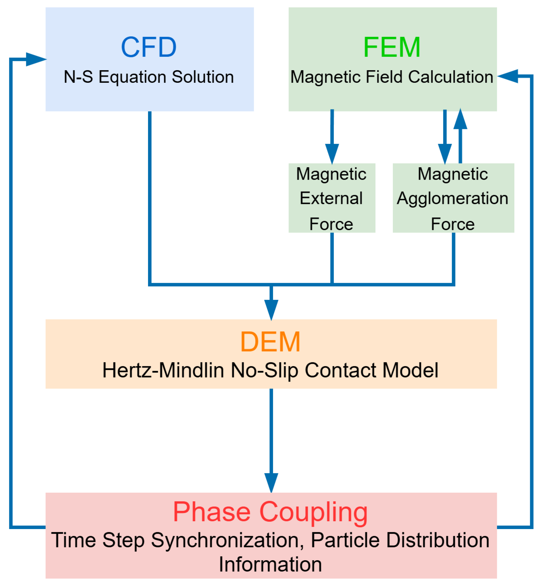
In this section, a multi-field dynamic coupling simulation and computational platform of FEM, CFD, and DEM is established. The platform is used to simulate and analyze the migration, aggregation, and accumulation processes of thousands of interacting micrometer-diameter magnetic particles in a fluid environment. It can also predict the generation, fracture, combination, and reconstruction processes of aggregates, among others. The framework of the dynamic model is shown in Figure 1.

Figure 1. Framework for multi-field dynamic coupling model.

The CFD-DEM coupling simulation adopts the Euler–Lagrange model and is realized through the coupling connection of the FLUENT-EDEM dual platforms. FLUENT uses the finite volume method to calculate the flow field and drag force. EDEM uses the Discrete Element Method to calculate the forces during particle collisions and solves the dynamic equations of particles to obtain the motion of particles. On this basis, COMSOL5.6 Multiphysics is used to solve the background magnetic field, and the magnetic field data are imported into a magnetic force program written in C++ language, which is then connected to the API interface of EDEM. In this way, the external magnetic field force and magnetic interaction force on the particles are solved, and finally the FEM-CFD-DEM dynamic coupling simulation is achieved.

2.1. Model of the Particle Phase

The DEM is used to calculate the particle phase. The forces acting on and the motion of the magnetic particles in the fluid under the action of the magnetic field are described by Newton’s second law, which can be expressed as follows:

$${\displaystyle \frac{\mathrm{d}}{\mathrm{d}t}}\left(m_{p}v\right)=F_D+F_g+F_{mi}+F_c+F_{ext},$$

(1)

where $m_p$ is the mass of the particle, kg; $\mathit{v}$ is the velocity of the particle, m/s; $\mathit{t}$ is the time, s; $F_D$ is the fluid drag force, N; $F_g$ is the apparent gravity, N; $F_{mi}$ is the magnetic field force, N; $F_c$ is the collision force between particles, N; $F_{ext}$ refers to other acting forces such as van der Waals force, Bassett lifting force, etc. In fact, in the single fiber trap particle model, $F_{ext}$ is negligible as it has little effect on the particles compared with the main forces under the sorting process conditions [9]. Then, Equation (1) can be simplified as follows:

$${\displaystyle \frac{\mathrm{d}}{\mathrm{d}t}}\left(m_{p}v\right)=F_D+F_g+F_{mi}+F_c,$$

(2)

The DEM uses the Hertz–Mindlin no-slip contact model to deal with collisions. This model belongs to the soft-sphere model and includes the normal force equation and the tangential force equation. The normal force $F_n$ includes the normal contact force $F_n^c$ and the normal damping force $F_n^d$, which can be expressed by the formula as follows:

$$F_n=F_n^c+F_n^d={\displaystyle \frac{4}{3}}{E}^{\ast }\sqrt{R^{\ast }}{{\delta }_n}^{{\displaystyle \frac{3}{2}}}-2\sqrt{{\displaystyle \frac{5}{6}}}\beta \sqrt{S_n{m}^{\ast }}{v}_n^{\mathit{rel}},$$

(3)

where $E^{\ast }$ is Young’s modulus, Pa; $R^{\ast }$ is the equivalent contact radius, m; ${\delta }_n$ is the normal overlap, m; $m^{\ast }$ is the equivalent mass, kg; $v_n^{\mathit{rel}}$ is the normal component of the relative velocity of the two particles, m/s; $S_n$ is the normal stiffness, N/m; and $\beta$ is the coefficient of restitution, dimensionless.

The tangential force $F_t$ includes the tangential contact force $F_t^c$ and the tangential damping force $F_t^d$, which can be expressed as follows:

$$\begin{gathered} F_t=F_t^c+F_t^d=-S_t{\delta }_t-2\sqrt{{\displaystyle \frac{5}{6}}}\beta \sqrt{S_t{m}^{\ast }}{v}_t^{\mathit{rel}}, \\ {S}_t=8G^{\ast }\sqrt{R^{\ast }{\delta }_n}, \end{gathered}$$

(4)

where $S_t$ is the tangential stiffness, N/m; G* is the shear modulus, Pa; ${\delta }_t$ is the tangential overlap, m; and $v_t^{\mathit{rel}}$ is the tangential relative velocity, m/s.

2.2. CFD Model of the Fluid

The fluid drag force $F_D$ is solved according to Stokes’ law, where the velocity of the fluid is solved by the CFD method. The Navier–Stokes (N-S) equations of the flow field can be expressed by the Mass Conservation Equation and Momentum Conservation Equation as follows:

$${\displaystyle \frac{\mathsf{\partial }\rho }{\mathsf{\partial }t}}+\nabla ·\left(\rho v\right)=0,$$

(5)

$$\rho \left({\displaystyle \frac{\mathsf{\partial }v}{\mathsf{\partial }t}}+\left(v·\nabla \right)v\right)=-\nabla p+\mu {\nabla }^{2}v+\rho g,$$

(6)

where $\rho$ is the density of the fluid, kg/m³; $v$ is the velocity of the flow field, m/s; $\mathit{t}$ is the time, s; $p$ is the fluid pressure, Pa; $\mu$ is the dynamic viscosity of the fluid, Pa·s; and $g$ is the acceleration due to gravity, m/s². In Equation (5), the first term on the right side is the pressure gradient, the second term is the viscous force, and the third term is the gravitational force. $\nabla$ refers to the Vector differential operator, Nabla operator, or Del operator.

2.3. FEM of the Magnetic Field

The FEM is used to solve the magnetic field. The solution of the magnetic field is based on Ampere’s circuital law and is described by the Maxwell–Ampere equation:

$${\mathit{\oint }}_{c}B·\mathrm{d}l={\mu }_0{{\displaystyle \int }}_s\left(J+{\displaystyle \frac{\partial D}{\partial t}}\right)·\mathrm{d}a,$$

(7)

where $B$ is the magnetic induction intensity, T; $\mathrm{d}l$ is the vector of the infinitesimal line element, m; $J$ is the current density passing through the curved surface S, A/m²; $D$ is the electric displacement, C/m²; $\mathrm{d}a$ is the vector of the infinitesimal surface element, m²; and ${\mu }_0$ is the magnetic permeability of vacuum, with ${\mu }_0=4\pi \times {10}^{-7}$, H/m.

The magnetic force $F_m$ acting on the magnetic particles in the magnetic field can be divided into two parts: the external magnetic field force and the magnetic agglomeration force, expressed as follows:

$$F_m=F_{me}+F_{mi},$$

(8)

where $F_{me}$ is the external magnetic field force, N; $F_{mi}$ is the vector of the magnetic agglomeration force, N.

The formula for solving $F_{me}$ can be expressed as follows [10]:

$$\left\{\begin{array}{l}{F}_{me}=2\pi {r_p}^3{\mu }_0{\mu }_{r}K\nabla H^2\\ K={\displaystyle \frac{{\mu }_{rp}-{\mu }_r}{{\mu }_{rp}+2{\mu }_r}}\end{array}\right.,$$

(9)

where $r_p$ is the radius of the particle, m; ${\mu }_{rp}$ and ${\mu }_r$ are the relative magnetic permeabilities of the magnetic particle and the fluid medium, respectively, dimensionless; and $H$ is the magnetic field strength of the external magnetic field of the particle, A/m.

3. Model of Magnetic Agglomeration Force

3.1. Dynamic Multi-Dipole Magnetic Moment Algorithm

In the fixed dipole model, only the effect of the external magnetic field is considered when calculating the dipole moment. For linear magnetic materials, their dipole moment can be expressed as follows:

$${\rm M}={\displaystyle \frac{4}{3}}\pi a^3{\chi }_{eff}{B}_0(r),$$

(10)

where ${\rm M}$ is the magnetic dipole moment, A·m²; $a$ is the particle radius, m; ${\chi }_{eff}$ is the effective magnetic susceptibility, dimensionless; $B_0(r)$ is the magnetic field intensity of the external magnetic field in which the particle is located, T; and $r$ is the position vector of the particle itself.

As shown in Figure 2, according to the theory of magnetization in a static magnetic field, the additional magnetization field generated after a substance is magnetized will be superimposed with the external magnetic field to form a new magnetic field environment. This new magnetic field will exert an additional effect on the magnetic dipole and generate a new torque. Since the magnetic dipoles at different positions are in different magnetic field environments, they are affected differently, which causes changes in the distribution and orientation of the magnetic dipoles and in turn leads to changes in the magnetic dipole moment. For example, N magnetic particles (nonlinear isotropic materials) are randomly placed in a non-uniform external magnetic field $B_0\left(r\right)$, and the position vectors of the particles are represented ${\mathit{r}}_n$ (n = 1, 2, 3,…, N). These magnetized particles can be described by a magnetic dipole moment $M_n$ at the position ${\mathit{r}}_n$ of the particle, and this magnetic dipole moment will also generate an additional magnetization magnetic field $B_a\left(r_n,r\right)$. $B_a\left(r_n,r\right)$ refers to the magnetization magnetic field generated by the magnetic moment at the n-th particle under the influence of $B_0\left(r\right)$, and $r_n$ is the position vector of the n-th particle that interacts with the current particle.

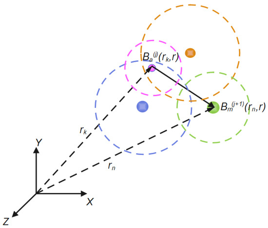
Figure 2. Schematic diagram of magnetic agglomeration solution.

Based on the fixed dipole model, a multi-magnetic dipole model has been developed. This model takes into account that the magnetic field $B_a\left(r_n,r\right)$ of other dipole particles will interfere with the magnetic field distribution around other particles, and its magnetic dipole moment can be expressed as follows:

$$M_n={\displaystyle \frac{4}{3}}\pi a^3{\chi }_{eff}\left[B_0\left(r\right)+{\displaystyle \sum _{\mathrm{k}=1,k\ne n}^N{B}_a\left(r_k,r\right)}\right],$$

(11)

In the multi-magnetic dipole model, the magnetic dipole moment changes once. In reality, after other particles are also magnetized, they will continue to affect the magnetic dipole moment of the original particles. The question is how to iterate repeatedly to reach a relatively stable state. Based on the multi-magnetic dipole model, the change in the magnetic dipole moment is solved through multiple iterative cycles to improve the accuracy of the interaction force between particles. By utilizing the linear superposition property of the magnetic field, the total superimposed magnetic field at the position ${\mathit{r}}_n$ of the n-th particle after the first cycle can be obtained as follows:

$${B_m}^{\left(1\right)}\left(r_n,r\right)=B_0\left(r\right)+{\displaystyle \sum _{k=1,k\ne n}^N{B_a}^{\left(0\right)}\left(r_k,r\right)}, \hspace{0.33em}\hspace{0.33em}\hspace{0.33em}n=1,\hspace{0.33em}2,\hspace{0.33em}3\dots ,N,$$

(12)

where ${B_m}^{\left(1\right)}(r_n,r)$ represents the first cycle adjustment of the local magnetic field at the location of the n-th particle. After this adjustment, the local magnetic field will generate a new local dipole moment ${M_n}^{\left(1\right)}$, and the additional magnetic field generated by this new dipole moment will be updated and corrected accordingly to ${B_a}^{\left(1\right)}(r_n,r)$.

Similarly, the other N-1 particles also undergo the same dynamic cycle process, and the magnetic fields at all particles are dynamically adjusted. This is the entire process of the first dynamic cycle correction of the magnetic field and the dipole moment, which covers all particles. Repeating this cycle in this way, and by analogy, the superimposed local magnetic field at the position ${\mathit{r}}_n$ of the n-th particle after the (j + 1)-th cycle is as follows:

$${B_m}^{\left(j+1\right)}\left(r_n,r\right)=B_0\left(r\right)+{\displaystyle \sum _{k=1,k\ne n}^N{B_a}^{\left(j\right)}\left(r_k,r\right)}, \mathrm{n}=1,\hspace{0.33em}2,\hspace{0.33em}3\dots ,N,$$

(13)

${B_m}^{\left(j+1\right)}\left(r_n,r\right)$ is the superimposed total magnetic field at the position $r_n$ of the n-th particle after the (j + 1)-th cycle, and ${B_a}^{\left(j\right)}\left(r_k,r\right)$ is the corrected additional magnetic field of the k-th particle after the j-th cycle. The influence of the other N − 1 particles on the magnetic field at the position of the n-th particle leads to the (j + 1)-th correction of the local magnetic field at the position of the n-th particle. The corrected magnetic field will magnetize to produce a new dipole moment ${M_n}^{\left(j+1\right)}$, and the new dipole moment will generate a new magnetic field ${B_a}^{\left(j+1\right)}\left(r_n,r\right)$. Here, j = 0 indicates that there is no correction for the magnetic field and the dipole moment, and j = 1, 2, 3, …, N represents the number of cycles of the magnetic dipole moment and the additional magnetized magnetic field. Since the magnetic dipole moment and the additional magnetized magnetic field can be repeatedly cycled and corrected, it is necessary to determine that the range of variation ${\displaystyle \frac{\left|M_n^{(j+1)}-M_n^{(j)}\right|}{\left|M_n^{(j)}-M_n^{(j-1)}\right|}}=A_{tol}$ of the local magnetic field (dipole moment) of the particle serves as the termination condition for the cycle.

In order to improve the calculation speed, the condition for the start of the cycle can be in the form of the maximum radius of the magnetic interaction force. Each magnetic particle influences each other within a region of the interaction distance, and the magnetic interaction distance depends on the external magnetic field, as well as the size and material of the particles. Referring to the maximum interaction distance of particles simulated by N.K. Lampropoulos et al. [11], E.G. Karvelas et al. [12], and others, the magnetic moments are only calculated for the interaction between particles within the distance range, and the particles outside the distance range will be automatically rejected by the algorithm, as shown in Figure 3.

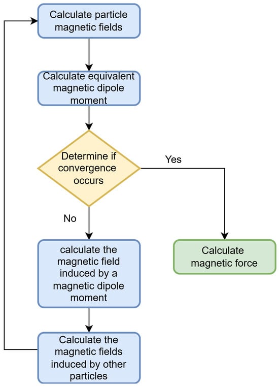
Figure 3. Schematic diagram of the iterative algorithm for magnetic particle clusters.

3.2. Calculation of Magnetic Agglomeration Force

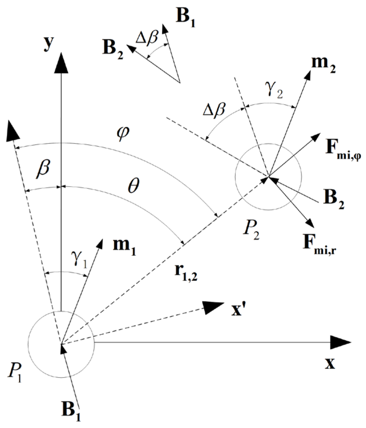
The calculation model of the magnetic agglomeration force $F_{mi}$ between magnetic particles is shown in Figure 4. According to electrodynamics, the magnetic potential energy $U$ between two magnetic particles can be written as follows:

$$U={\displaystyle \frac{{\mu }_0}{4\pi }}{\displaystyle \frac{1}{r^3}}\left[m_1·m_2-3\left(m_1·\widehat{r}\right)\left(m_2·\widehat{r}\right)\right],$$

(14)

where $m_1$ and $m_2$ are the magnetic dipole moments generated after the two magnetic particles are magnetized, with the unit of A/m²; $\widehat{r}$ is the unit vector in the direction of the distance vector between the two particles.

Figure 4. Schematic diagram of magnetic agglomeration solution.

In the interaction theory of magnetic dipoles, the interaction between magnetic particles can be described by a magnetic potential energy function. For any two magnetic particles, since the magnetic field intensity vector $B_2$ passing through a certain particle and the direction vector $r_{1,2}$ of the particle must be coplanar, a two-dimensional relative coordinate system can always be found. In this coordinate system, the axial component $F_{mi,r}$ and the tangential component $F_{mi,\phi }$ of the magnetic interaction force can be calculated. The two magnetic particles are denoted as $P_1$ and $P_2$, respectively. A local two-dimensional relative coordinate system Ox′y′ with $P_1$ as the origin is established, the direction of the magnetic field at the position of $P_1$ is the y′-axis, and the axis perpendicular to the y′-axis and on the same side of $r_{1,2}$ is the x′-axis. By solving the magnetic potential energy $U$ between any two magnetic particles in the magnetic field, the magnetic agglomeration force $F_{mi}$ between the two magnetic particles is obtained as follows:

$$F_{mi}=F_{mi,r}{r}^{\prime }+F_{mi,\phi }\phi =-{\displaystyle \frac{\delta U}{\delta r}}{r}^{\prime }-{\displaystyle \frac{1}{r}}{\displaystyle \frac{\delta U}{\delta \phi }}\phi ,$$

(15)

where $r^{\prime }$ and $\phi$ are the radial and angular unit vectors in the polar coordinate system, respectively; $r$ is the distance between the two particles, with the unit of m; and $\phi$ is the included angle between the direction vector $r_{1,2}$ of the particles and the y′-axis of the polar coordinates, with the unit of rad.

Through coordinate transformation, the radial and axial magnetic interaction forces in the relative coordinate system can be transformed into the vector of the magnetic interaction force in any two-dimensional or three-dimensional physical space coordinate system. The derivation of the three-dimensional magnetization model is based on the two-dimensional model. Its core point is to utilize the characteristics of the parallel magnetic field. A plane is established through two particle points and a magnetic field vector, and then the two-dimensional derivation results are applied on this two-dimensional plane. As shown in Figure 5, based on the conventional coordinate system, the calculation plane S can be drawn in the three-dimensional space by selecting the two central points of the calculated particle pair and the direction of the magnetic field.

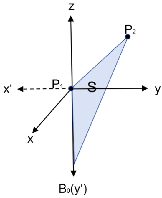
Figure 5. Schematic diagram of three-dimensional calculation of magnetic interaction force.

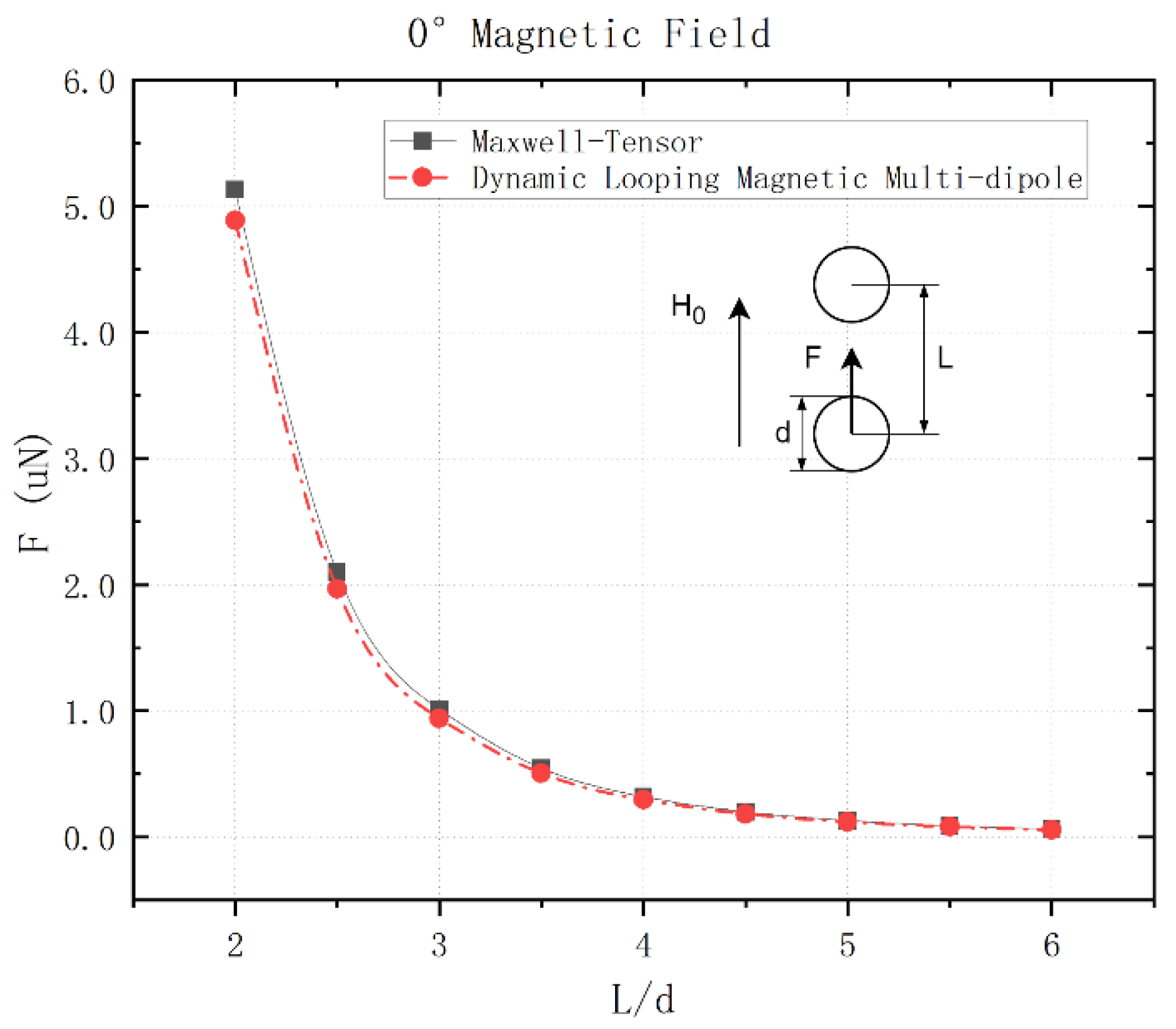
To verify the method of dynamic cyclic mutual dipole magnetic moments, taking the case of two magnetic particles suspended in a non-magnetic fluid and subjected to a uniform magnetic field as an example, the interaction force between the particles obtained by using the dynamic magnetic moment algorithm is compared with the interaction force between the particles calculated by the Maxwell tensor method. For two spherical magnetic particles located in a uniform magnetic field, the distance between the centers of the two particles is given. Except for the size of the square cavity filled with a non-magnetic fluid, all the variables of the magnetic problems used to verify this method are dimensionless. As shown in Figure 6, the interaction force between the particles is given when the spacing (L) is 2 to 6 times the particle diameter (d). The abscissa L/d is the ratio of the particle spacing to the particle diameter, and the ordinate is the interaction force between the particles, where the unit of the force is μN.

Figure 6. The interaction force between the particles in different L/d conditions.

In Figure 6, as L/d decreases, the difference in the calculated interaction force between the particles by different methods gradually increases, and the difference in the interaction force between the particles increases from 0.0051 μN to 0.246 μN. When L/d = 2, the error of the calculated value by the dynamic magnetic moment method compared with the calculation result of the Maxwell stress tensor method is only 5.0%, and it gradually decreases and remains stable as the particle spacing increases.

3.3. Results and Comparison of the Model Simulation

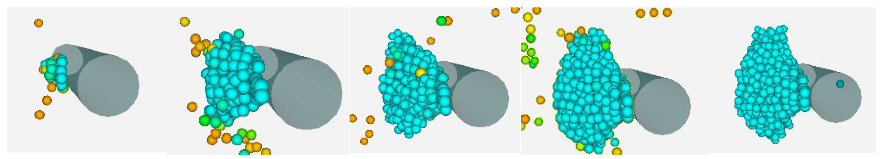
Regarding the problem of aggregate deposition under the dominance of magnetic force, observing the dynamic process of particle accumulation on a single-filament medium under unsteady-state conditions can help us better understand the dynamic characteristics of the deposition of micron-sized particles on a cylindrical single-filament medium, as well as the influencing laws of the structure and morphology of the deposited body. As shown in Figure 7, it is the accumulation process of the deposition adsorption body in a parallel configuration, from adsorption on the smooth surface to the formation of a dynamic saturated layer.

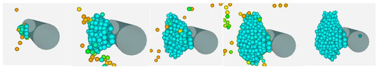
Figure 7. Particle aggregation sedimentary structures under parallel configuration.

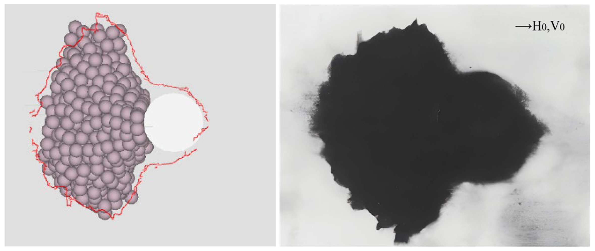
As shown in Figure 8, we also compared the simulation results of the dynamic model with the experimental observation results of Watson et al. [13]. Table 1 lists several key simulation parameters, and the parallel configuration and weakly magnetic particles were selected. The aggregation evolution contour curves of the experimental observation results were extracted and compared with the simulation results of the dynamic model. They are very similar in the flow-facing area.

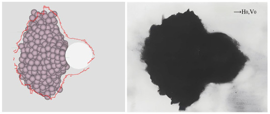
Figure 8. Comparison between the simulation results of the dynamic model and the experimental observation results.

Table 1. Key parameter settings for experiments and simulations.

Content	Parameter	Definition
Particle properties	Material type	Wolframite
	Magnetic susceptibility	3400 × 10−6 (SI)
	Density	6.63 g/cm3
	Particle diameter	10 μm
Wire medium properties	Material	Nickel
	Magnetic susceptibility	600
	Diameter	10 μm
Parameter	Reynolds number Re	6
	Background magnetic field strength	1 T

4. Conclusions

This paper takes the separation process of magnetic particles as the research object and focuses on developing and improving a multi-field dynamic coupling simulation model based on discrete dynamics. This model is used to analyze the influence of the interactions between particles, fluid–solid coupling, and the magnetic field on dynamic behaviors such as aggregation, migration, and dispersion during the separation process. By applying the particle dynamics method, the relationship between the magnetic field conditions and the motion characteristics of particles is revealed from the perspective of the separation mechanism.

In the calculation of the magnetic field force, the magnetic dipole theory is introduced, and the magnetic field force is divided into the external magnetic field force and the magnetic aggregation force for separate calculations. A solid-phase magnetic field force model is established and embedded into the DEM 2018 simulation software. At the same time, it is coupled with the CFD software to obtain a dynamic calculation model for magnetic particles. In this model, the k-ε turbulence model is used for the liquid phase. For the solid phase, both the field force exerted by the physical field on the particles and the non-contact interaction force between particles are taken into account.

The proposed coupling model adopts a dynamic cyclic multi-dipole magnetic moment algorithm to calculate the magnetic interaction force between particles. Compared with the traditional static dipole magnetic moment algorithm, the error of the calculated value by the dynamic magnetic moment method compared with the calculation result of the Maxwell stress tensor method is only 5.0% (when L/d = 2 in Figure 6), and the error gradually decreases and remains stable as the particle spacing increases. So, it has higher accuracy and a wider application range. Moreover, the P-E magnetization model suitable for a two-dimensional uniform magnetic field is further improved and optimized to make it applicable to a three-dimensional gradient magnetic field, making it more consistent with the actual application scenarios. The simulation results of the dynamic model are in agreement with the experimental observation results of Watson and other researchers.

References

- Yuan, Z. Magnetoelectric Separation; Metallurgical Industry Press: Beijing, China, 2011. (In Chinese) [Google Scholar]
- Xie, P.; Wang, F.; Tang, D.; Zhao, M.; Dai, H. Research Progress in the Application of Numerical Simulation in Magnetic Separation. Nonferrous Met. (Miner. Process. Sect.) 2023, 6, 9–18. (In Chinese) [Google Scholar]
- Murariu, V. Simulating a Low Intensity Magnetic Separator Model (LIMS) using DEM, CFD and FEM Magnetic Design Software. In Proceedings of the 4th International Computational Modelling Symposium, Singapore, 20–22 June 2025; Minerals Engineering International: Cornwall, UK, 2013; pp. 301–314. [Google Scholar]
- Lindner, J.; Menzel, K.; Nirschl, H. Simulation of magnetic suspensions for HGMS using CFD, FEM and DEM modeling. Comput. Chem. Eng. 2013, 54, 111–121. [Google Scholar] [CrossRef]
- Hu, Y. Analysis on simulation of magnetic separation process using dynamic coupled FEM, CFD and DEM model. Nonferrous Met. (Miner. Process. Sect.) 2016, 68–72, 82. (In Chinese) [Google Scholar]
- Wu, J.; Yue, X.; Guo, X.; Dai, S.; Zhang, M.; Ren, J. Simulation of Three Product Magnetic Separation Column Process Simulation Based on FEM, CFD and DEM Coupling. Met. Mine 2024, 2, 225–231. (In Chinese) [Google Scholar]
- Pinto-Espinoza, J. Dynamic Behavior of Ferromagnetic Particles in a Liquid-Solid Magnetically Assisted Fluidized Bed (MAFB): Theory, Experiment, and CFD-DPM Simulation. Ph.D. Thesis, Oregon State University, Corvallis, OR, USA, 2003. [Google Scholar]
- Chen, J.; An, R.; Shu, J.; Li, D.; Liu, X.; Mao, Y.; Chen, J.; Gao, H.; Lyu, W.; Meng, F. Study on motion of multi-component ferromagnetic particles with modified magnetization model. Chin. J. Theor. Appl. Mech. 2024, 56, 740–750. (In Chinese) [Google Scholar]
- Zhang, L.A.; Diao, Y.F.; Zhuang, J.W.; Zhou, F.S.; Shen, H.G. Performance of single fiber collection PM 2.5 under different magnetic field forms in the iron and steel industry. Chin. J. Eng. 2020, 42, 154–162. [Google Scholar]
- Rosensweig, R.E. Fluidization: Hydrodynamic stabilization with a magnetic field. Science 1979, 204, 57–60. [Google Scholar] [CrossRef] [PubMed]
- Lampropoulos, N.K.; Karvelas, E.G.; Papadimitriou, D.I.; Sarris, I.E. Computational study of the optimum gradient magnetic field for the navigation of spherical particles into targeted areas. J. Phys. Conf. 2015, 637, 012038. [Google Scholar] [CrossRef]
- Karvelas, E.G.; Lampropoulos, N.K.; Sarris, I.E. A numerical model for aggregations formation and magnetic driving of spherical particles based on OpenFOAM. Comput. Methods Programs Biomed. 2017, 142, 21–30. [Google Scholar] [CrossRef] [PubMed]
- Watson, J.H.P.; Li, Z. A study on mechanical entrapment in HGMS and vibration HGMS. Miner. Eng. 1991, 4, 815–823. [Google Scholar] [CrossRef]
Disclaimer/Publisher’s Note: The statements, opinions and data contained in all publications are solely those of the individual author(s) and contributor(s) and not of MDPI and/or the editor(s). MDPI and/or the editor(s) disclaim responsibility for any injury to people or property resulting from any ideas, methods, instructions or products referred to in the content. |
© 2025 by the authors. Licensee MDPI, Basel, Switzerland. This article is an open access article distributed under the terms and conditions of the Creative Commons Attribution (CC BY) license (https://creativecommons.org/licenses/by/4.0/).