Effect of Temperature on First-Order Decay Models and Uncertainty Analysis for the Prediction of Methane Emissions in a Landfill Located in the Urban Area of Oaxaca City, Mexico

Abstract

Landfill disposal continues to be the most economically viable municipal solid waste (MSW) management practice in many countries, including Mexico. Landfills are the third-largest source of methane emissions from human activity, a fact that has significant implications for the environment and human health. Due to the difficulty in experimentally quantifying methane emissions, mathematical models have been employed to predict gas emissions. In this work, three first-order decay models were implemented to estimate methane emissions in a landfill located in the metropolitan area of Oaxaca City, Mexico. Each model incorporated a Van’t Hoff–Arrhenius-type approach for calculating the reaction rate constant. Additionally, an uncertainty analysis of the models was presented, applying Monte Carlo simulations with triangular and log-normal distributions. The results show that the simple model exhibited the best predictive performance. For 2020, the simple model estimated 3,488,392.1 m³ of methane at a temperature of 46 °C, 3,509,625.1 m³ of methane at 47 °C, and 3,530,850.2 m³ of methane at 48 °C. The Monte Carlo simulation with a log-normal distribution exhibited more robust and natural process behavior. For the simple model, the mean was 3,486,946.03, the median was 3,487,154.73, and the standard deviation was 212,095.95. The LandGEM model exhibited more linear methane generation behavior, and the uncertainty analysis confirmed that this model had the lowest predictive capability of the three proposed models.

1. Introduction

Due to their impact on the environment and on health, there has been a notable interest in predicting gas emissions from landfills. This is because these emissions are considered greenhouse gases. These gaseous emissions are caused by complex chemical reactions, which are significantly affected by temperature [1,2]. According to [3], temperature affects the physical, chemical, biological, and mechanical properties and behavior of wastes and liner materials in landfills. In the work of [4], the authors studied the effect of temperature on methane generation from solid waste using samples from several landfills in California and New York, with temperatures ranging from 21 °C to 48 °C. These authors highlight that a temperature of 41 °C was identified as the optimal condition for short-term methane production. The conclusions of this study indicate that these temperature variations caused slight changes in the microbial population, and that the energy activation value was higher than in previous studies.

In the work of [5], the authors implemented the CLEEN (Capturing Landfill Emissions for Energy Needs) model to estimate methane emissions from a landfill, taking into account precipitation and ambient temperature. To develop their model, the authors used 27 laboratory-scale reactors and calculated the values of the reaction rate constant k as functions of waste composition, annual rainfall, and temperature. Likewise, they estimated k from data obtained from 11 landfills with conventional operation. The k values showed significant variations. When comparing the methane emissions estimated by the CLEEEN, LandGEM, and IPCC models, the authors found that the CLEEN model more accurately estimated four out of the six cases studied. Moreover, the reported k values in the literature vary widely, ranging from 0.01 to 0.51 per year [6,7].

The use of land surface temperature for monitoring landfills has also been investigated by many authors. In the work of [8], the authors analyzed Landsat images to understand the thermal behavior of landfills. Interestingly, temperature fluctuations demonstrated a periodic cycle due to the seasonal change. Also, in landfills, emission of methane can somehow be estimated since there is indeed a moderate correlation between methane emissions and the land surface temperature [9]. The land surface temperature can be indirectly implemented in situations where experimental data in landfills are unavailable.

Heat is generated because of complex biochemical reactions and degradation of organic components in solid waste. Ref. [10] investigated heat generation in municipal solid waste landfills. Waste temperatures diminished from the elevated levels at the landfill base but remained above ground temperatures. Heat content was found to align with exponential growth and decay curve relationships based on climatic and operational conditions. Heat generation was ascertained through the law of heat conduction utilizing one-dimensional heat transfer analysis. The authors mentioned that the maximum reported temperatures generally varied from approximately 40 to 65 °C and were observed within the middle one-third depth to over one-half depth of landfills with total waste heights of approximately 20 to 60 m.

It is well known that temperature is a factor that affects anaerobic consortia cell metabolism, which influences the kinetic behavior of waste decomposition [1,2,11]. The Arrhenius model and the Van’t Hoff–Arrhenius relationship can be used to understand the effect of temperature on the gas decomposition process in landfills, since parameter k affects first-order kinetic models. Based on the Arrhenius description, Ref. [12] proposed an extended model to account for the effect of temperature on the estimation of the parameter k for modeling the anaerobic co-digestion of waste. These authors propose using the Van’t Hoff–Arrhenius equation to relate the reaction rate constant at a given temperature to the reaction rate constant at a reference temperature.

When mathematical models are used to predict phenomena, it is important to analyze the models’ uncertainty, which is a measure of doubt about a model’s proper functioning linked to its parameters, since simplifications and assumptions are typically employed. Furthermore, in systems such as landfills, the lack of information is a recurring problem. The IPCC recognizes that uncertainty is inherent in first-order decay models [13], indicating that parameters and input data are the main sources of uncertainty [14]. Therefore, having sufficient, high-quality information is important for obtaining representative and reliable results. However, in many landfills, information is limited and incomplete, making it difficult to obtain accurate parameter values. This translates into uncertainty in the results. To address this issue, Monte Carlo simulation has been proposed, which is a statistical approach that allows for predicting the uncertainty associated with the model. In this type of methodology, multiple values for the parameters of interest are randomly generated, and the calculation is repeated thousands of times until a range of probable outcomes is established that better represents the system [15].

An uncertainty analysis was proposed by [16], who compared the results of first-order models and included a Monte Carlo uncertainty analysis for each model parameter. The authors considered a normal probability distribution, a triangular distribution, and a log-normal distribution. The authors mentioned that Monte Carlo estimates allowed for an adequate analysis of uncertainty, and that the type of distribution affected the uncertainty range. According to [17], methane estimation in landfills is subject to uncertainty due to various factors: variability in waste composition, waste age, the chosen method, and parameters such as the decomposition rate and methane generation potential.

In this work, we solved three models to estimate the methane emissions in Oaxaca City. The effect of temperature was assessed by considering the Van’t Hoff–Arrhenius approach. The uncertainty of models was assessed by Monte Carlo simulations.

2. Theory

2.1. Van’t Hoff–Arrhenius

Arrhenius Equation (1) describes the relationship between the rate constant (k) of a chemical reaction, the temperature (T), and the activation energy (Ea). The Arrhenius equation is expressed as:

$$k=A·exp\left({\displaystyle \raisebox{1ex}{${-E}_a$}\!\left/ \!\raisebox{-1ex}{$RT$}\right.}\right)$$

(1)

where

k is the rate constant of the reaction [year⁻¹].

A is the pre-exponential factor (or frequency factor), which represents the frequency of molecular collisions with the proper orientation.

E_a is the activation energy [J/mol]

R is the universal gas constant [J/mol K]

T is the temperature [K].

The Arrhenius equation demonstrates that the rate of a reaction increases exponentially with temperature and decreases as the activation energy increases. The Van’t Hoff–Arrhenius equation is commonly used in environmental engineering applications because it is easier to calibrate with experimental data, and it is expressed as in Equation (2):

$$k_T=k_{ref}·{\theta }^{\left(T-T_{ref}\right)}$$

(2)

where

• $k_T$ is the rate constant of the reaction at temperature T.
• $k_{ref}$ is the rate constant of the reaction at Tref (20 °C or 25 °C).
• $\theta$ (theta) is the temperature coefficient, an empirical value that indicates the effect of temperature on the reaction rate. Typically, for biological processes such as anaerobic digestion, its value ranges from 1.03 to 1.10.
• T is temperature of the system (°C).
• $T_{ref}$ is the temperature of reference (°C).

2.2. The Monte Carlo Simulation

Monte Carlo simulation is a statistical technique used to analyze uncertainty and variability in complex systems. It is based on performing repeated random sampling. In each sample, the input factor and the model parameters can take on different values. These values are simulated based on the distribution of the input factor values and the parameters [18].

We are interested in analyzing the decomposition rate of waste. The values of k exhibit a range of variability. In the Monte Carlo simulation, two distributions are employed: the triangular distribution and the log-normal distribution. The selection of the probability distribution is linked to the characteristics of the parameter being simulated. The log-normal distribution is used to estimate the uncertainty of environmental parameters, primarily because it ensures that values are always positive, which appropriately represents phenomena with skewness and a long tail [19]. According to [20], the probability density function of x follows the behavior expressed by the following equation:

$$f_{\mathcal{x}}\left(\mathcal{x}\right)={\displaystyle \frac{1}{\sigma \mathcal{x}\sqrt{2\pi }}}\mathcal{e}-{\displaystyle \frac{1}{2{\sigma }^2}}{\left[\ln \left(\mathcal{x}\right)-\mu \right]}^2\mathcal{x}\ge 0$$

(3)

where

$$\mu =\mathbb{E}\left[\mathit{ln}\left(\mathcal{x}\right)\right]$$

(4)

$$\sigma =\sqrt{Var\left[\ln \left(\mathcal{x}\right)\right]}$$

(5)

• $\mu$ = Mean of the logarithm.
• $\sigma$ = Standard deviation.
• $\mathbb{E}$ = Expected value.
• Var = Variance.

The values of s in the log-normal distribution can vary between 1.0, 0.5, and 0.25. With s equal to 1, the distribution exhibits high dispersion and is skewed to the right. With s equal to 0.5, the dispersion decreases, showing values far from the mean, and with s equal to 0.25, the x values are closer to 1, resulting in an asymmetric, narrow distribution.

3. Materials and Methods

3.1. Landfill of Zaachila, Oaxaca

The landfill is in the town of Zaachila, Oaxaca, at approximately 16°57′ north latitude and 96°44′ west longitude. This landfill operated for several years and was closed in 2022. Solid waste from 24 municipalities in the Oaxaca City metropolitan area was disposed of at this site. The landfill is a controlled site with an arrangement of confinement cells. In this way, the site has infrastructure for the collection and treatment of leachate. On site, the waste is compacted and covered by tractors and backhoe loaders. The landfill covers an area of approximately 17 hectares. The available data for the generation of solid waste (Ton/year) correspond to the period from 1991 to 2012, whereby an extrapolation for the period from 2012 to 2022 is carried out via the FORECAST function in Microsoft ^® Excel for Mac (version 16.99, Microsoft 365). Excel’s FORECAST function allows you to forecast future values using past values. The main forecasting equation is:

$$y=a+bx$$

(6)

where

$$a=\overline{y}-\overline{bx}$$

(7)

$$b={\displaystyle \frac{\sum \left(x-\overline{x}\right)\left(y-\overline{y}\right)}{\sum {\left(x-\overline{x}\right)}^2}}$$

(8)

where

• x: independent value;
• y: predicted value.

The ETS algorithm, which uses exponential smoothing for time series, was used in the forecast.

In 1991, 52,554.72 tons/year were reported, and in 2022, 108,202 tons/year were estimated. The composition of solid waste was extracted from [21].

3.2. Weather Data

The Oak Ridge National Laboratory Distributed Active Archive Center shares a dataset called DAYMET [22], from which monthly weather data from 1980 to 2021 can be obtained. Additionally, a mean temperature for southwest Mexico is taken from [23]. DAYMET shows grid-based estimates of average high and low temperatures, as well as total rainfall, measured at a space resolution of 1 km by 1 km. The monthly average temperature is calculated by taking the mean of the highest and lowest temperatures. Based on these data, an average temperature for southern Mexico of 25 °C can be considered. Furthermore, according to the area’s climatological information, the Zaachila landfill is located in a hot, semi-arid climate [24].

Based on the information above, a reference temperature was considered. The Van’t Hoff–Arrhenius equation was used to estimate the values of k at three temperature levels.

3.3. Mathematical Models for Predictiing Methane Emissions

Three decay models were analyzed: the simple model, the modified simple model, and the LandGEM model (Table 1). All three models were implemented in Microsoft ^® Excel for Mac (version 16.99, Microsoft 365).

Table 1. Models of first-order decay.

Model	Equation		Index of Symbols
Simple model	$G=W{ L}_{0 }k e^{-k \left(t-t_i\right)}$	(9)	G = Generation of methane (m3/year); W = Mass of waste (Tons); L0 = Potential of generation of methane (m3/Ton); t = Time after waste placement (years); ti = Lag time (between placement and start of generation; k = First-order rate constant (year−1).
Modified simple model	$G=W L_0 {\displaystyle \frac{k+s}{s}}\left[1-e^{-s\left(t-t_i\right)}\right]\left[k{ e}^{-k \left(t-t_i\right)}\right]$	(10)	G = Generation of methane (m3/year); W = Mass of waste (Tons); L0 = Potential of generation of methane (m3/Ton); t = Time after waste placement (years); ti = Lag time (between placement and start of generation; k = First-order rate constant (year−1); s = Constant of the phase of first order.
LandGEM model	$Q_{{CH}_4}={\displaystyle \sum _{i=1}^n}{\displaystyle \sum _{j= 0.1}^1}k L_0\left({\displaystyle \frac{M_i}{10}}\right)e^{-k{t}_{i j}}$	(11)	QCH4 = Annual methane generation in the year of the calculation (m3/year); n = (year of the calculation) − (initial year of waste acceptance); i = 1-year time increment; j = 0.1-year time increment; k = Methane generation rate (year−1); L0 = Potential methane generation capacity (m3/Mg); Mi = Mass of waste accepted in the ith year (Mg); tij = Age of the jth section of waste mass accepted in the ith year (decimal of year).

According to the EPA (2008), the values of L₀ vary from 6 to 270 m³/Mg, and a predetermined value of 100 m³/Mg data is obtained from experimental studies of 40 landfills [25].

Assumptions of the models:

Solid waste corresponds to municipal solid waste.

The site works under anaerobic conditions.

The waste composition remains constant throughout the study period.

The averaged temperature approach is considered for the landfill.

3.4. Uncertainty of Models

For the implementation of the Monte Carlo simulation, two distributions were employed: the triangular distribution and the log-normal distribution. The triangular distribution is used when there is a known relationship between variable data, but data availability is limited for a comprehensive analysis. It is characterized by its dependence on the maximum, minimum, and most likely values, and is commonly used in simulations and decision analysis when the data generation process is unknown, which is why it is also known as the unknown distribution [26].

For an input $x_i$, with a triangular distribution and limits a+ and a−, we have:

$$x_i={\displaystyle \frac{a_{+}+a_{-}}{2}}$$

(12)

The standard uncertainty is calculated as:

$$u_{\left(x_i\right)}={\displaystyle \frac{a_{+}+a_{-}}{\sqrt{24}}}$$

(13)

According to [27], k can be calculated as:

$$\mathrm{k}={3.2\times 10}^{-5}\left(\mathrm{x}\right)+0.01$$

(14)

where

• x = Average annual precipitation (mm).

This expression allowed us to calculate a central value for k. For this parameter, the average annual precipitation at the station closest to the landfill was considered, which was 484.8 mm/year, so k_mean = 0.026 year⁻¹. The values for k_min, k_mean, and k_max were as follows: 0.0247, 0.0261, and 0.0273 year⁻¹, respectively.

To estimate a performance indicator from a simulation, a dataset Yi … Yn was considered, obtained through N independent simulation runs. Yn was obtained through N independent simulation runs. Each value Yi represents the outcome observed in the i-th run and is assumed to be independent and identically distributed according to the probability function f. The objective of this simulation was to estimate the expected value of the variable of interest.

The Monte Carlo simulation was performed in Python 3.11, executed in Google Colab. The np.random.lognormal function was used for the log-normal distribution, and np.random.triangular for the triangular distribution from the NumPy library [28]. A total of 10,000 interactions were generated; this number of iterations was carried out in accordance with the law of large numbers. This principle of probability theory states that as the number of repetitions of a random experiment increases, the average of the outcomes tends to approach the expected value. For each value of k, the methane generation estimate was calculated using the equations of the first-order decay models. The relative error versus the observed data was calculated to identify fits with a 5% error. Additionally, the mean was calculated, which corresponded to the sum of all possible values, weighted by their frequencies [29].

4. Results

4.1. Mathematical Models

Figure 1 shows the methane generation curves using the simple model. The experimental value measured in 2020 serves as the benchmark for the models. The values of k calculated for temperatures of 46, 47, and 48 °C were as follows: 0.02588, 0.02613, and 0.02640. The Van’t Hoff–Arrhenius approach allows for the inclusion of the temperature effect.

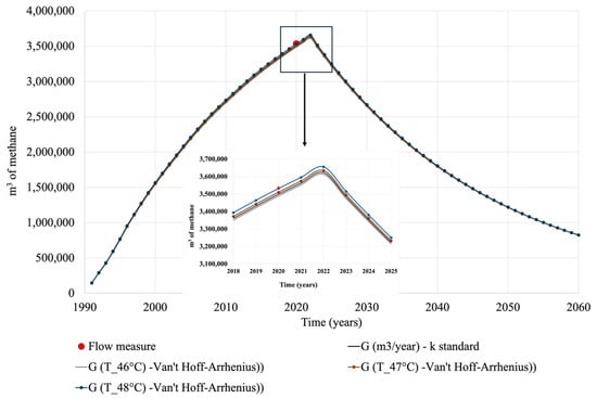
Figure 1. Results for simple model.

Figure 1 shows the methane generation calculated by the simple model. Methane generation followed an exponential growth pattern until 2022, when the landfill was closed by the government of the State of Oaxaca. The methane emissions calculated for the period from 1990 to 2020 were substantial, which underscores the relevance of this research. In 2020, at an average temperature of 46 °C, 3,488,392.1 m³ of methane was calculated; at 47 °C, 3,509,625.1 m³ of methane; and at 48 °C, 3,530,850.2 m³ of methane was estimated. The experimental data measured in 2020 was 3,534,870.2 m³, meaning the simple model closely approximated the measured value when a temperature of 48 °C was used. After reaching peak emissions (year 2020), these models predicted a decline. The decay was calculated until 2060, revealing significant amounts of methane. In the case of the 48 °C prediction scenario, emissions in 2060 will be 824,005.64 m³. As can be seen in Figure 1, stabilizing emissions will take several more years. The amount of methane that will be emitted in the coming years is considerable.

In Figure 1, experimental values are also presented (red point). These data were obtained in 2020 from a report generated by the company “Sistemas de Ingeniería y Control Ambiental S.A. de C.V.” This measurement necessitated flow sampling at the entrances of the biogas extraction wells within the landfill. The company conducted a sampling of the biogas flow in the headers of the extraction system. The experimental data were measured at ambient conditions (20 °C and 1 atm). The behavior of the curves was consistent with the waste decomposition process, and the use of the Van’t Hoff–Arrhenius approach seemed correct.

In Figure 2, the curves of the modified simple model are presented, considering the Van’t Hoff–Arrhenius expression for the k values. We observe that this model overpredicts the experimentally measured value. For this model, the same temperatures as in the simple model are considered, namely 46, 47, and 48 °C. This model shows that at the beginning of the process (from 1990 onward), the emission is slow, as the curve exhibits a smooth slope, but after 1994 it begins to grow exponentially, overpredicting the experimental value for 2020. After this peak, the classic exponential decay begins. By 2060, this model predicts the emission of approximately 1,000,000 m³ of methane. These predictions are very important, as landfills are known to be the third-largest source of methane emissions from human activities in countries such as the United States. Despite the overestimation, this second model also confirms that stabilizing emissions will take several decades, which necessitates monitoring for the coming decades.

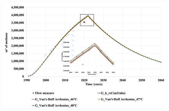
Figure 2. Modified simple model.

In Figure 3, we present the LandGEM model’s prediction. The model greatly overestimates experimental values (the flow measure is the red point). Likewise, we observe that the curve’s behavior exhibits more linear growth and decay trends. LandGEM has been studied by other authors, and they have documented this overprediction behavior, primarily due to the need to input specific data for each landfill.

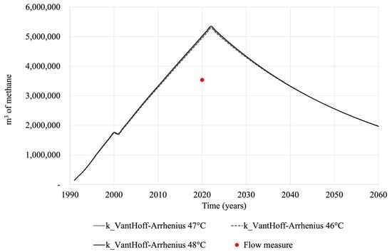
Figure 3. LandGEM model.

The emissions calculated for the landfill’s closing year (2022) at the three different temperatures of interest were 5,283,186.65 m³ of methane (46 °C), 5,319,154.81 m³ of methane (47 °C), and 5,355,226.13 m³ of methane (48 °C). By 2060, this model predicts emissions of approximately 2,000,000 m³ of methane. This overprediction has been reported by various authors. According to [30], LandGEM neglects waste categorization in its assessments, and a significant limitation of the LandGEM model is its presumption of uniform waste composition, which disregards the variability in organic content and degradation rates among different waste layers, resulting in possible inaccuracies in methane generation predictions. In the work [31], the authors developed machine learning techniques to reduce the error in their predictions. These authors found the KNN (k-nearest neighbors) algorithm reduced the prediction error by 54% compared to the LandGEM results. In the work of [14], the authors identify an overestimation of 20% for the LandGEM model in a landfill located in Denmark. In the case of the Audebo landfill (Denmark), LandGEM initially overestimated by almost 40%.

In any of the models, it is shown that stabilizing methane emissions will take several decades. These types of processes have both short- and long-term effects, so it is important to quantify and implement measures to capture or control emissions.

According to [32], optimum temperature ranges for the growth of mesophilic and thermophilic bacteria involved in waste decomposition were identified to be 35 to 40 °C and 50 to 60 °C. The temperatures used for methane estimation were within the ranges reported by different authors.

4.2. Uncertainty

For the simple model, two distributions are implemented: the triangular and the normal log. Results are displayed in Table 2.

Table 2. Statistical results for the simple model.

Simple Model
	Triangular Distribution	Log-Normal Distribution
Mean	3,499,745.10	3,486,946.03
Median	3,501,519.71	3,487,154.73
Standard deviation	43,386.93	212,095.95
P2.5	3,414,736.06	3,071,201.18
P97.5	3,578,947.72	3,902,842.57

The simulation with the triangular distribution yields a mean of 3,499,745.10 m³ and a median of 3,501,519.71 m³, both of which indicate a distribution close to symmetry (Figure 4a), suggesting good model precision in the face of variability in parameter k. The standard deviation is 43,386.93; this result indicates moderate variability in the simulations. According to the 2.5 and 97.5 percentiles, 95% of the simulated results fall within the range of 3,414,736.06 to 3,578,947.72. The experimentally measured flow falls within the 95% confidence interval. The 95% confidence intervals for the mean are estimated at 3,498,894.73 to 3,500,595.47, with a margin of error of ±850.37.

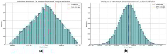
Figure 4. Monte Carlo simulations for simple model: (a) triangular distribution; (b) log-normal distribution.

On the other hand, the simulation results with the log-normal distribution show positive skewness (Figure 4b), with a mean of 3,486,946.03, which is lower than the median of 3,487,154.73, and a bias toward values higher than the mean. This indicates a higher probability that the methane estimate will be above the mean. The 2.5 and 97.5 percentiles at the 95% confidence level lie in the range of 3,071,201.18 to 3,902,842.57. The experimentally measured methane value falls within the 95% confidence interval and lies in the central part of the curve, indicating that the model with this distribution adequately captures the landfill measurement. The 95% confidence intervals for the mean are estimated to be from 3,482,789.02 to 3,491,103.03, with a margin of error of ±4157.00. This log-normal distribution exhibits natural skewness, which offers the advantage of robustness in modeling exponentially decaying processes.

With regard to the modified simple model, Table 3 presents the results obtained from Monte Carlo simulations using triangular and log-normal distributions.

Table 3. Statistical results for the simple modified model.

Simple Modified Model
	Triangular Distribution	Log-Normal Distribution
Mean	3,758,307.27	3,746,620.19
Median	3,760,372.00	3,742,050.94
Standard deviation	55,368.94	271,158.81
P2.5	3,650,340.97	3,307,577.75
P97.5	3,859,899.50	4,198,709.54

For the modified simple model with the triangular distribution, the estimated mean emissions are 3,758,307.27 m³, with a median of 3,760,372.00 m³. The method calculates a standard deviation of 55,368.94. The 2.5 and 97.5 percentiles are at 3,650,340.97 and 3,859,899.50, respectively, indicating a narrow range and lower dispersion. The shape of the curve indicates symmetry with a well-defined central peak (Figure 5a), a limitation inherent to the method since it is based on bounding a maximum value, a minimum value, and the mode. The experimental value falls outside the 95% confidence interval, as it lies below the lower limit, indicating that the model overestimates methane emission values. The 95% confidence intervals for the mean are estimated at 3,757,222.06 and 3,759,392.48, with a margin of error of ±1085.21.

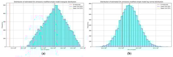
Figure 5. Monte Carlo simulations for the simple modified model: (a) triangular distribution; (b) log-normal distribution.

The log-normal distribution improves the prediction, as the experimental value is closer to the center of the bell curve, but a slight overestimation of emissions is once again confirmed. This model exhibits a mean of 3,746,620.19 m³, a median of 3,742,050.94 m³, and a standard deviation of 271,158.81, which is higher than that of the triangular distribution, indicating more dispersed values. Figure 5b shows a curve with asymmetry and positive skew, characteristic of this type of distribution, with the highest concentration of frequencies near the mean. The experimental value lies within the 2.5 and 97.5 percentiles, which correspond to 3,307,577.75 and 4,198,709.54, respectively. The modified simple model overestimates methane emissions.

Table 4 shows the Monte Carlo simulation results for methane estimation using the LandGEM model, with triangular and log-normal distribution.

Table 4. Statistical results for LandGEM model.

LandGEM Model
	Triangular Distribution	Log-Normal Distribution
Mean	4,615,725.38	4,609,967.45
Median	4,618,065.87	4,610,323.11
Standard deviation	57,219.07	279,671.58
P2.5	4,503,609.10	4,061,515.06
P97.5	4,720,183.71	5,158,158.89

Monte Carlo simulations confirm the results obtained from the Arrhenius–Van’t Hoff decay models: a very high overprediction by the LandGEM model. The triangular distribution shows a mean of 4,615,725.38 m³ and a median of 4,618,065.87 m³. The standard deviation is 57,219.07. Figure 6a describes the important prediction aspect of this model. Regarding the 2.5 and 97.5 percentiles, they range from 4,503,609.10 to 4,720,183.71, respectively. The experimental value lies outside the prediction range, indicating that the LandGEM model overestimates methane emission values. The 95% confidence intervals for the mean are estimated to range from 4,614,603.90 to 4,616,846.85, with an error of ±1121.47.

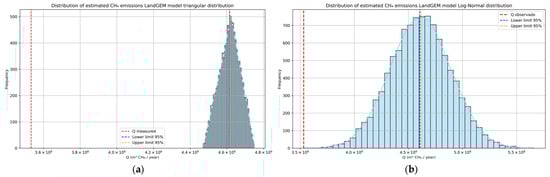
Figure 6. Monte Carlo simulations for LandGEM model: (a) triangular distribution; (b) log-normal distribution.

On the other hand, in the log-normal distribution, despite exhibiting more robust behavior, overestimation of the experimental value is also observed. The mean is estimated to be lower than that of the triangular distribution, with a median of 4,610,323.11 m³ and a standard deviation higher than that of the triangular distribution (279,671.58). Figure 6b shows a slightly asymmetrical curve with a rightward skew. In this distribution, the experimental value lies within the 2.5 and 97.5 percentiles, which range from 4,061,515.06 to 5,158,158.89. The 95% confidence intervals range from 4,604,485.99 to 4,615,448.92, respectively, with an error of ±5481.46.

According to the results, it is observed that the type of probability distribution chosen for the simulation influences the shape of the distribution and the robustness of the simulations. According to our results, the simple model provides a better prediction of the experimental value. The modified simple model slightly overestimates this experimental measurement, and the LandGEM model significantly overestimates the experimental value.

5. Discussions

The three first-order decay models predict methane emissions in a landfill located in the metropolitan area of Oaxaca City. They are selected based on data analysis and accessibility. Figure 1, Figure 2 and Figure 3 in the manuscript show the decay dynamics after the last waste disposal in 2022. Each model has significant structural differences that reflect the variation in estimated emissions.

The three models share two fundamental parameters: methane generation potential (L0) and methane generation rate (k) [6,7]. However, the simple model primarily considers k and Lo. It describes a single-phase decomposition process, as it considers one category of waste. This model includes the exponential component negatively affected by the k parameter and by time. It also considers a lag time, which corresponds to the time between waste disposal and the start of biogas generation.

The modified simple model incorporates an additional parameter, known as the first-order rise phase constant, into the model structure. This phase constant controls the onset of methane generation, so this model assumes that methane generation is initially low, then increases to a maximum, before decreasing exponentially [8,9]. This behavior coincides with what the IPCC [10] mentions, which indicates the existence of a delay time associated with anaerobic decomposition, which represents the period from waste disposal to the start of methane generation, usually around 6 months or 0.5 year⁻¹ (IPCC, 2006). It also includes in the exponential both the phase constant and the reaction constant. This model is also classified as single-phase because it considers one category of waste.

The LandGEM model has a different structure from previous models. This model is based on a first-order degradation equation that divides the mass into ten parts. This model assumes that landfill gas is composed of approximately 50% methane and 50% carbon dioxide, with additional, relatively low concentrations of other atmospheric pollutants. The model assumes that gas generation is fastest at the beginning, shortly after the waste is deposited, once anaerobic conditions are established [11]. The structure of this model is considered a double summation: the first to integrate the fractions within the year (j) and the second to add up the years of deposit [11].

The simple model is useful when information is limited, as few parameters are needed to solve it. The modified simple model is a bit more complex, but it requires information to establish the phase constant. The LandGEM model is a reference model, but its accuracy depends largely on the quality of the annual residue data and parameters. According to Da Silva et al. [12], this model was developed using standard US data, which results in low accuracy when applied to other sites.

In the work of Colomer et al. [13], it is mentioned that the first-order and modified models overestimated biogas generation, as they had a mean relative error of 32% and 30%, respectively. Unlike our results, the simple and modified simple models were closest to the 2020 measurement value. This is because the values of k and L0 were estimated according to local conditions, data that coincide with Krause et al. [14], who mentioned that single-phase models can adequately predict methane generation as long as the input parameters are calculated.

6. Conclusions

In this study, three mathematical models were solved for predicting methane emissions from a landfill located in the metropolitan area of Oaxaca City. The models were the simple model, the modified simple model, and LandGEM model. To account for the effect of landfill temperature, the Arrhenius–Van’t Hoff term was included, which has been applied to environmental systems. The three first-order decay models generally captured the behavior of the emissions. The reaction rate constant k was calculated using the Van’t Hoff–Arrhenius approach. Likewise, Monte Carlo simulations were implemented to analyze the uncertainty of the proposed models.

According to our results, the simple model exhibited the best predictive capability for methane emissions, which was confirmed by Monte Carlo simulation. The modified simple model predicted the emission behavior; however, it slightly overestimated the experimental emissions, whereas the LandGEM model exhibited a more linear methane generation pattern and significantly overestimated the experimental value. Monte Carlo simulations with a log-normal distribution exhibited more robust behavior, with more natural skewness.

Predicting methane emissions is a difficult task because the biochemical reactions that occur in landfills are numerous, simultaneous, and complex. However, the simple Van’t Hoff–Arrhenius approach yielded acceptable results. The use of mathematical models is useful for this type of application, since a bottleneck in many landfills is the scarcity of experimental data. In the case of the State of Oaxaca, continuous and extensive monitoring is required, as the amounts of methane emitted over time are considerable and should be discussed in greater detail.

References

- Gou, C.; Yang, Z.; Huang, J.; Wang, H.; Xu, H.; Wang, L. Effects of temperature and organic loading rate on the performance and microbial community of anaerobic co-digestion of waste activated sludge and food waste. Chemosphere 2014, 105, 146–151. [Google Scholar] [CrossRef] [PubMed]
- Nie, E.; He, P.; Zhang, H.; Hao, L.; Shao, L.; Lü, F. How does temperature regulate anaerobic digestion? Renew. Sustain. Energy Rev. 2021, 150, 111453. [Google Scholar] [CrossRef]
- Yesiller, N.; Hanson, J.L. Analysis of Temperatures at a Municipal Solid Waste Landfill. In Proceedings of the Ninth International Waste Management and Landfill Symposium, Sardinia, Italy, 6–10 October 2003. [Google Scholar]
- Hartz, K.E.; Klink, R.E.; Ham, R.K. Temperature Effects: Methane Generation from Landfill Samples. J. Environ. Eng. Div. 1982, 108, 629–638. [Google Scholar] [CrossRef]
- Karanjekar, R.V.; Bhatt, A.; Altouqui, S.; Jangikhatoonabad, N.; Durai, V.; Sattler, M.L.; Hossain, S.; Chen, V. Estimating methane emissions from landfills based on rainfall, ambient temperature, and waste composition: The CLEEN model. Waste Manag. 2015, 46, 389–398. [Google Scholar] [CrossRef]
- Amini, H.R.; Reinhart, D.R.; Mackie, K.R. Determination of first-order landfill gas modeling parameters and uncertainties. Waste Manag. 2012, 32, 305–316. [Google Scholar] [CrossRef]
- Ishigaki, T.; Van Chung, C.; Sang, N.N.; Ike, M.; Otsuka, K.; Yamada, M.; Inoue, Y. Estimation and field measurement of methane emission from waste landfills in Hanoi, Vietnam. J. Mater. Cycles Waste Manag. 2008, 10, 165–172. [Google Scholar] [CrossRef]
- Yan, W.Y.; Mahendrarajah, P.; Shaker, A.; Faisal, K.; Luong, R.; Al-Ahmad, M. Analysis of multi-temporal landsat satellite images for monitoring land surface temperature of municipal solid waste disposal sites. Environ. Monit. Assess. 2014, 186, 8161–8173. [Google Scholar] [CrossRef]
- Ishigaki, T.; Yamada, M.; Nagamori, M.; Ono, Y.; Inoue, Y. Estimation of methane emission from whole waste landfill site using correlation between flux and ground temperature. Environ. Geol. 2005, 48, 845–853. [Google Scholar] [CrossRef]
- Yeşiller, N.; Hanson, J.L.; Liu, W.-L. Heat Generation in Municipal Solid Waste Landfills. J. Geotech. Geoenviron. Eng. 2005, 131, 1330–1344. [Google Scholar] [CrossRef]
- Maldonado-Saeteros, S.; Baquerizo-Crespo, R.J.; Gómez-Salcedo, Y.; Pérez-Ones, O.; Pereda-Reyes, I. Influence of temperature on kinetics and hydraulic retention time in discontinuous and continuous anaerobic systems. Environ. Eng. Res. 2023, 28, 210442. [Google Scholar] [CrossRef]
- Wang, S.; Hovland, J.; Bakke, R. Modeling and simulation of lab-scale anaerobic co-digestion of MEA waste. Model. Identif. Control. 2014, 35, 31–41. [Google Scholar] [CrossRef]
- IPCC. Directrices del IPCC de 2006 Para Los Inventarios Nacionales de Gases de Efecto Invernadero 3.1. Available online: https://www.ipcc-nggip.iges.or.jp/public/2006gl/spanish/vol5.html (accessed on 28 July 2023).
- Krause, M.J.; Chickering, G.W.; Townsend, T.G. Translating landfill methane generation parameters among first-order decay models. J. Air Waste Manag. Assoc. 2016, 66, 1084–1097. [Google Scholar] [CrossRef] [PubMed]
- Rafey, A.; Siddiqui, F.Z. Modelling and simulation of landfill methane model. Clean. Energy Syst. 2023, 5, 100076. [Google Scholar] [CrossRef]
- Szemesova, J.; Gera, M. Uncertainty analysis for estimation of landfill emissions and data sensitivity for the input variation. In Greenhouse Gas Inventories: Dealing with Uncertainty; Jonas, M., Nahorski, Z., Nilsson, S., Whiter, T., Eds.; Springer: Dordrecht, The Netherlands, 2011; pp. 37–54. [Google Scholar] [CrossRef]
- Rasouli, M.A.; Karimpour-Fard, M.; Machado, S.L. An assessment of the uncertainties of methane generation in landfills. J. Air Waste Manag. Assoc. 2025, 75, 464–482. [Google Scholar] [CrossRef] [PubMed]
- Kissell, R.L. Chapter 8—Nonlinear Regression Models. In Algorithmic Trading Methods, 2nd ed.; Kissell, R.L., Ed.; Academic Press: Cambridge, MA, USA, 2021; pp. 197–219. [Google Scholar] [CrossRef]
- Andersson, A. Mechanisms for log normal concentration distributions in the environment. Sci. Rep. 2021, 11, 16418. [Google Scholar] [CrossRef]
- López, J.O.; Londoño, N.A. Probabilidad y Estadística. Fondo Editorial EIA. 2019. Available online: https://elibro-net.bibliotecaipn.idm.oclc.org/es/ereader/ipn/125705?page=58 (accessed on 25 September 2025).
- Merab, P.B.N.; Sadoth, S.T.; Isidro, B.J.S. First-Order Decay Models for the Estimation of Methane Emissions in a Landfill in the Metropolitan Area of Oaxaca City, Mexico. Waste 2025, 3, 14. [Google Scholar] [CrossRef]
- Thornton, M.M.; Shrestha, R.; Wei, Y.; Thornton, P.E.; Kao, S.-C. Earth Science Data Systems. Daymet: Daily Surface Weather Data on a 1-km Grid for North America, Version 4 R1 NASA Earthdata; Earth Science Data Systems, NASA; 16 June 2025. Available online: https://www.earthdata.nasa.gov/data/catalog/ornl-cloud-daymet-daily-v4r1-2129-4.1 (accessed on 23 September 2025).
- Arellano-González, J.; Juárez-Torres, M. Temperature and quarterly economic activity: Panel data evidence from Mexico. Environ. Dev. Econ. 2025, 27, 1–21. [Google Scholar] [CrossRef]
- INEGI. Climatología. Available online: https://www.inegi.org.mx/temas/climatologia/ (accessed on 20 October 2025).
- EPA. Background Information Document for Updating AP42 Section 2.4 for Estimating Emissions from Municipal Solid Waste Landfills Science Inventory US EPA. Available online: https://cfpub.epa.gov/si/si_public_record_report.cfm?Lab=NRMRL&dirEntryId=198363 (accessed on 27 July 2023).
- Kissell, R.L. Chapter 5—Probability and Statistics. In Algorithmic Trading Methods, 2nd ed.; Kissell, R.L., Ed.; Academic Press: Cambridge, MA, USA, 2021; pp. 129–150. [Google Scholar] [CrossRef]
- Park, J.-K.; Chong, Y.-G.; Tameda, K.; Lee, N.-H. Methods for determining the methane generation potential and methane generation rate constant for the FOD model: A review. Waste Manag. Res. J. A Sustain. Circ. Econ. 2018, 36, 200–220. [Google Scholar] [CrossRef]
- Harris, C.R.; Millman, K.J.; van der Walt, S.J.; Gommers, R.; Virtanen, P.; Cournapeau, D.; Wieser, E.; Taylor, J.; Berg, S.; Smith, N.J.; et al. Array programming with NumPy. Nature 2020, 585, 357–362. [Google Scholar] [CrossRef]
- Kleine, L.L. Bioestadística. Ph.D. Thesis, Editorial Universidad Nacional de Colombia, Bogotá, Colombia, 2012. Available online: https://elibro-net.bibliotecaipn.idm.oclc.org/es/ereader/ipn/129822?page=34 (accessed on 6 October 2025).
- Ali, T.; Bari, Q.H.; Rafizul, I.M. Field validation of predictive model for greenhouse gas emissions from unsanitary landfill. Clean. Eng. Technol. 2025, 29, 101086. [Google Scholar] [CrossRef]
- Saeedi, M.; Mohammadi, M.; Esmaeili, N.; Niri, F.F.; Gol, H. Optimizing LandGEM model parameters using a machine learning method to improve the accuracy of landfill methane gas generation estimates in the United States. J. Environ. Manag. 2025, 373, 124029. [Google Scholar] [CrossRef]
- Tchobanoglous, G.; Kreith, F. (Eds.) Handbook of Solid Waste Management, 2nd ed.; McGraw-Hill Education: New York, NY, USA, 2002; Available online: https://www.accessengineeringlibrary.com/content/book/9780071356237 (accessed on 23 September 2025).
Disclaimer/Publisher’s Note: The statements, opinions and data contained in all publications are solely those of the individual author(s) and contributor(s) and not of MDPI and/or the editor(s). MDPI and/or the editor(s) disclaim responsibility for any injury to people or property resulting from any ideas, methods, instructions or products referred to in the content. |
© 2025 by the authors. Licensee MDPI, Basel, Switzerland. This article is an open access article distributed under the terms and conditions of the Creative Commons Attribution (CC BY) license (https://creativecommons.org/licenses/by/4.0/).