Intelligent Monitoring of Lost Circulation Risk Based on Shapelet Transformation and Adaptive Model Updating

Abstract

As unconventional hydrocarbon resources gain increasing importance, the risk of lost circulation during drilling operations has also grown significantly. Accurate and reliable risk diagnosis methods are essential to ensure safety and operational efficiency in complex drilling environments. This study proposes a novel lost circulation risk monitoring framework based on time-series shapelet transformation, integrated with Generative Adversarial Network (GAN)-based data augmentation and real-time model updating strategies. GANs are employed to synthesize diverse, high-quality samples, enriching the training dataset and improving the model’s ability to capture rare or latent lost circulation signals. Shapelets are then extracted from the time series using a supervised shapelet transform that searches for discriminative subsequences maximizing the separation between normal and lost-circulation samples. Each time series is subsequently represented by its minimum distances to the learned shapelets, so that critical local temporal patterns indicative of early lost circulation can be explicitly captured. To further enhance adaptability during field applications, a real-time model updating mechanism is incorporated. The system incrementally refines the classifier using newly incoming data, where high-confidence predictions are selectively added for online updating. This strategy enables the model to adjust to evolving operating conditions, improves robustness, and provides earlier and more reliable risk warnings. We implemented and evaluated Support Vector Machine (SVM), k-Nearest Neighbors (kNNs), Logistic Regression, and Artificial Neural Networks (ANNs) on the transformed datasets. Experimental results demonstrate that the proposed method improves prediction accuracy by 6.5%, measured as the accuracy gain of the SVM classifier after applying the shapelet transformation (from 84.7% to 91.2%) compared with using raw, untransformed time-series features. Among all models, SVM achieves the best performance, with an accuracy of 91.2%, recall of 90.5%, and precision of 92.3%. Moreover, the integration of real-time updating further boosts accuracy and responsiveness, confirming the effectiveness of the proposed monitoring framework in dynamic drilling environments. The proposed method offers a practical and scalable solution for intelligent lost circulation monitoring in drilling operations, providing a solid theoretical foundation and technical reference for data-driven safety systems in dynamic environments.

1. Introduction

As global energy demand continues to grow, drilling activities in the oil and gas industry are rapidly expanding into deeper and more geologically complex drilling environments. During the extraction process, factors such as unpredictable formations, high-pressure reservoirs, and the configuration of drilling tools often give rise to complex downhole incidents [1]. Among these, lost circulation is one of the most frequent and challenging events encountered in drilling operations. If not identified and addressed promptly, lost circulation can lead to severe drilling fluid losses, wellbore instability, formation damage, and even well control complications—posing serious threats to personnel safety, equipment integrity and the surrounding ecosystem. With the advent of the Fourth Industrial Revolution, driven by technologies such as artificial intelligence, and the increasing maturity of emerging technologies like AI-based decision systems [2] and expert systems [3] built on big data, new opportunities are emerging for intelligent diagnosis and risk prediction. In particular, advances in computing power and the development of machine learning algorithms offer promising solutions for improving the accuracy and timeliness of lost circulation monitoring in drilling environments. Alkinani et al. [4] applied neural networks to predict lost circulation in fractured formations before drilling and found that the Levenberg–Marquardt (LM) algorithm exhibited the best performance. Geng et al. [5] investigated the influence of formation conditions on lost circulation risk and used machine learning algorithms such as random forests to build predictive models capable of effectively identifying minor circulation losses. Abbas et al. [6] collected data related to drilling operation parameters, formation types, lithology, and drilling fluid properties and developed lost circulation classification models using neural networks and support vector machines (SVMs), with results showing that the SVM outperformed the neural network. Hou et al. [7] predicted the probability of different levels of lost circulation using neural networks based on geological features, drilling fluid properties, and drilling operational parameters. Shi et al. [8] employed intelligent algorithms such as random forests and SVM to construct predictive models for lost circulation, achieving a test accuracy of up to 90%. Pang et al. [9] developed an intelligent monitoring model for lost circulation based on a mixture density neural network, achieving a relative error of 7% and demonstrating good performance in field applications. Sun et al. [10] analyzed the relationship between drilling conditions, total pit volume, and outlet flow rate, and proposed an intelligent lost circulation diagnosis method that combines drilling parameters with a Bi-GRU model. Wu et al. [11] proposed an unsupervised time series autoencoder (BiLSTM-AE) model for intelligent monitoring of lost circulation, achieving an accuracy of 92.51%. Wu et al. [12] selected 12 parameters and introduced an improved extreme learning machine (IELM) model, achieving an F1 score (harmonic mean of precision and recall) of 97.22%. Moreover, the model trained with the optimal feature set demonstrated higher accuracy and faster convergence.

Despite recent advances in intelligent monitoring of lost circulation risks, key challenges remain—most notably the limited availability of labeled abnormal event data and poor model generalization across varying drilling conditions. The rarity of lost circulation events often results in insufficient training samples, leading to underfitting, overfitting, and reduced predictive accuracy. To address this, data augmentation using generative techniques have been introduced to simulate diverse lost circulation scenarios, enriching the dataset and improving model generalization. Meanwhile, shapelet-based time series transformation enables the extraction of critical temporal patterns from drilling data, offering clearer insight into the early evolution of circulation loss. In addition, incorporating a real-time model updating mechanism allows the system to adapt to dynamic operational conditions, thereby enhancing responsiveness and early warning accuracy. Collectively, these approaches significantly improve the accuracy, robustness, and adaptability of lost circulation prediction models—providing a strong foundation for safer and more intelligent drilling operations.

2. Methodology

2.1. Data Preprocessing

The data used in this study were collected from seven wells located in western and southwestern China, comprising comprehensive well-logging and drilling operation records. Initial preprocessing involved outlier detection using the box-plot method, followed by the removal of abnormal values. Missing values were imputed using the mean for continuous variables and the mode for categorical variables. Although this simple strategy may introduce bias in variance or slightly distort feature distributions, it was adopted due to the low proportion of missing data and the need for consistent preprocessing across heterogeneous drilling parameters. In addition, numerical features were normalized to a uniform scale to facilitate stable model training and improve convergence. To ensure rigorous model evaluation and prevent data leakage, the dataset was partitioned strictly at the well level. All data from a given well were assigned exclusively to either the training set or the testing set, ensuring that no well appeared in both subsets. This strategy avoids the model learning location-specific noise patterns and ensures that the evaluation reflects true generalization capability across different wells. Lost circulation event labels were then assigned by integrating drilling logs with expert-defined indicators, such as sudden decreases in total pit volume, sharp drops in standpipe pressure, and recorded loss severity levels. Through this process, a structured and location-independent dataset suitable for supervised model training and evaluation was obtained.

To reduce data redundancy and improve model efficiency, correlation analysis and feature selection were conducted. Here, correlation analysis means evaluating Pearson correlation coefficients among variables to identify weakly related or redundant features. The Pearson correlation coefficient was used to quantify the linear relationships between variables, which helped identify and eliminate weakly correlated or irrelevant features. This dimensionality reduction not only reduced computational complexity and memory requirements but also improved model training efficiency and prediction accuracy. The values of the Pearson coefficient range from −1 to +1, where values closer to ±1 indicate stronger linear relationships [13].

Based on correlation analysis and domain expertise, the following key parameters were selected for monitoring lost-circulation risks: outlet flow rate, total pit volume, standpipe pressure, rate of penetration (ROP), outlet mud density, and inlet mud density.

2.2. Generative Adversarial Network Data Augmentation

The Generative Adversarial Network (GAN), introduced by Goodfellow et al. in 2014 [14], is a class of deep learning models based on adversarial training. It consists of two neural networks—the generator and the discriminator—which are trained simultaneously in a minimax game framework. The generator attempts to produce data that mimic the real data distribution, while the discriminator strives to distinguish between real and generated data samples. The general architecture of a GAN model is illustrated in Figure 1, where the interaction between the generator and discriminator forms the basis of iterative learning and model improvement. GANs have demonstrated remarkable success in various data generation tasks, including image synthesis, speech generation, and text modeling, due to their ability to learn complex, high-dimensional data distributions. Their capability to generate realistic synthetic data makes them highly applicable in domains with limited or imbalanced datasets. Figure 1 illustrates the architecture of the generative adversarial network.

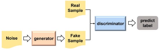
Figure 1. The Structure of Generative Adversarial Network.

In the context of lost circulation risk monitoring, the scarcity of labeled abnormal event data poses a significant challenge to the development of robust predictive models. Lost circulation events are relatively infrequent but highly impactful, and the resulting imbalance between normal and abnormal data can lead to underfitting, poor generalization, and reduced sensitivity to early-stage risk signals.

Zhou et al. applied CTGAN for tabular data generation in lost circulation monitoring and observed notable improvements in model performance [15]. However, CTGAN does not account for the sequential nature of drilling data. In contrast, a Recurrent Conditional Generative Adversarial Network (RCGAN) is capable of generating realistic multivariate time series that preserve both short-term fluctuations and long-term temporal dependencies, making it well suited for simulating drilling dynamics and lost-circulation trends [16]. RCGAN consists of a recurrent generator and a recurrent discriminator conditioned on auxiliary variables, enabling the model to capture temporal patterns and class-dependent characteristics within the data. During training, the generator produces synthetic sequences in the same temporal structure as the original drilling parameters, while the discriminator evaluates whether the sequence is real or generated under the given condition. This adversarial learning framework allows RCGAN to learn the underlying temporal distribution of drilling signals more effectively than conventional GANs that ignore time dependency. The synthetic time-series samples produced by RCGAN were used to augment the original drilling dataset, effectively increasing the diversity and representation of rare lost-circulation patterns. This augmentation process enhances the sensitivity and robustness of downstream classifiers in data-constrained environments.

To verify the quality of the generated data, we performed a distribution-level similarity assessment using t-SNE–based dimensionality reduction. As shown in Figure 2, the t-SNE projection of real and RCGAN-generated samples exhibits substantial overlap in the embedded space, indicating that RCGAN successfully captures the key statistical and structural characteristics of the original time-series data and provides credible synthetic samples for model training.

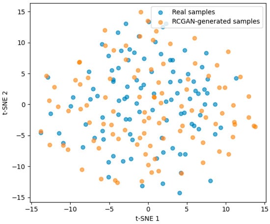
Figure 2. t-SNE visualization of real and RCGAN-generated samples.

2.3. Shapelet Transformation

Shapelet transformation is a feature extraction method used for processing time series data. Its purpose is to capture key patterns and trends within time series data to improve the performance of time series classification and pattern recognition tasks [17,18].

The essence of the transformation is to find the top k best shapelets, and then derive a new attribute for each shapelet, where the attribute value represents the distance from each case to a shapelet. In this context, k represents the predefined number of top-ranked shapelets chosen based on their discriminative power, where each shapelet is a short subsequence that best separates the normal and lost-circulation classes. The process is as follows:

In this study, candidate shapelets were generated by sliding windows of varying lengths over all training sequences. The minimum and maximum lengths were set to 20 and 80 sampling points, respectively, based on prior knowledge of the typical duration of early lost-circulation fluctuations in drilling parameters. For each candidate subsequence, its distance to a time series is defined as the minimum Euclidean distance between the subsequence and all same-length windows within the series.

To determine which shapelets are most informative, each candidate was evaluated using Information Gain, a commonly used supervised metric that quantifies how well a subsequence separates the two classes (normal vs. lost-circulation). Candidates were then ranked by their Information Gain scores, and highly redundant shapelets with similar distance profiles were removed. The parameter k represents the predefined number of top-ranked, non-redundant shapelets selected based on this criterion.

After selecting the top-k shapelets, each time series is transformed into a new feature vector, where each dimension corresponds to the minimum distance between the series and one shapelet. This transformation removes the temporal ordering but preserves discriminative local patterns, enabling the use of a wide range of machine-learning classifiers. Figure 3 shows example shapelets extracted from a representative dataset.

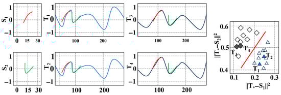
Figure 3. Two Shapelets Learned on a Particular Dataset.

2.4. Building Different Classifiers

To accurately assess lost circulation risk, multiple machine learning models were constructed and compared in this study to identify the most suitable classifier for drilling data. Different algorithms exhibit distinct modeling mechanisms and learning capabilities, enabling a more comprehensive understanding of the data characteristics. By analyzing their predictive behaviors on shapelet-transformed time series, the study aims to capture both linear and nonlinear patterns underlying lost circulation phenomena.

The selected models include Support Vector Machine (SVM), k-Nearest Neighbors (kNN), Logistic Regression, and Artificial Neural Networks (ANN). These algorithms represent a diverse set of approaches, covering statistical learning, distance-based learning, and neural computation paradigms. Their complementary strengths enhance the robustness and generalization ability of the proposed monitoring framework. The structure and working principles of each classifier are illustrated in Figure 3. Compared with relying on a single modeling approach, the use of multiple classifiers enables a more thorough exploration of the data and yields more accurate and reliable prediction results.

2.4.1. Support Vector Machine (SVM)

Support Vector Machine (SVM) is a supervised learning algorithm widely applied in classification and regression tasks [19]. The core idea of SVM is to find an optimal hyperplane in a high-dimensional space that maximizes the margin between different classes. By transforming input features into higher-dimensional spaces through kernel functions, SVM is able to handle both linearly separable and nonlinearly separable problems.

During training, SVM identifies support vectors, which are the most critical samples closest to the decision boundary. These support vectors determine the position and orientation of the optimal hyperplane. Kernel functions such as linear, polynomial, radial basis function (RBF), and sigmoid can be selected according to the problem characteristics, providing strong flexibility and adaptability.

SVM offers several advantages: it is effective in high-dimensional spaces, is robust to overfitting when the number of dimensions exceeds the number of samples, and has strong generalization ability. However, it may face computational challenges when applied to large-scale datasets, and the selection of kernel functions and hyperparameters significantly influences its performance.

2.4.2. k-Nearest Neighbors (kNN)

k-Nearest Neighbors (kNN) is a simple yet effective non-parametric algorithm widely used for classification and regression tasks [20]. The fundamental principle of kNN is based on the assumption that similar samples are likely to have similar labels. For a given query sample, kNN calculates its distance (commonly Euclidean, Manhattan, or Minkowski distance) to all training samples, identifies the k closest neighbors, and determines the predicted output based on their majority class or average value.

The advantages of kNN lie in its straightforwardness, ease of implementation, and the fact that it makes no assumptions about the underlying data distribution. Moreover, it can adapt to multi-class classification problems and is highly interpretable. However, its drawbacks include high computational cost in large-scale datasets due to the need for distance calculation, sensitivity to the choice of k value, and vulnerability to irrelevant or noisy features.

2.4.3. Logistic Regression

Logistic Regression is a classical statistical learning algorithm commonly used for binary classification problems [21]. Unlike linear regression, Logistic Regression introduces the logistic (sigmoid) function to map linear combinations of input features into probability values between 0 and 1. This probabilistic framework allows the model to output the likelihood of a sample belonging to a particular class.

The model parameters are estimated using maximum likelihood estimation (MLE), and regularization terms such as L1 (Lasso) and L2 (Ridge) can be applied to prevent overfitting. Logistic Regression is efficient, interpretable, and performs well when the relationship between features and outcomes is approximately linear.

Although its simplicity is an advantage, Logistic Regression has limitations in handling complex nonlinear relationships. In such cases, feature engineering or kernelized extensions may be required to improve performance.

2.4.4. Artificial Neural Networks (ANNs)

Artificial Neural Networks (ANNs) are a class of machine learning algorithms inspired by the structure and functioning of biological neural systems [22]. ANNs consist of layers of interconnected nodes (neurons), including input layers, one or more hidden layers, and output layers. Each neuron performs a weighted sum of inputs, followed by a nonlinear activation function such as sigmoid, tanh, or ReLU, enabling the network to capture complex and nonlinear patterns.

Training ANNs typically involves backpropagation and gradient descent optimization to minimize the loss function. With sufficient hidden units and layers, ANNs can approximate highly complex functions and demonstrate strong predictive power across a wide range of tasks. The strengths of ANNs include their ability to model nonlinear relationships, flexibility in handling diverse data types, and extensibility to deep learning architectures. However, ANNs require large training datasets, are computationally intensive, and may suffer from overfitting if not properly regularized. Despite these challenges, ANNs have achieved remarkable success in many real-world applications. In petroleum engineering studies, ANN performance is often evaluated through detailed error analysis and model validation procedures. For example, ANN-based prediction of reservoir permeability changes has demonstrated the importance of assessing model accuracy using metrics such as error distribution and convergence behavior [23]. Such practices provide valuable guidance for evaluating ANN reliability in lost-circulation risk diagnosis as well.

2.4.5. XGBoost

XGBoost is an efficient gradient-boosting algorithm widely used for classification and anomaly detection tasks. It builds an ensemble of decision trees in a stage-wise manner, where each new tree corrects the residual errors of the previous ones. Due to its ability to model nonlinear feature interactions and its built-in regularization, XGBoost offers strong generalization performance even on relatively small datasets [24].

For the shapelet-transformed feature space, XGBoost is particularly suitable because tree-based models naturally handle the distance-based features generated by shapelets and are resistant to noise and feature redundancy. Key hyperparameters—including the number of trees, learning rate, and maximum tree depth—were tuned through grid search with 5-fold cross-validation to achieve a balance between accuracy and computational efficiency. The optimized XGBoost model serves as a strong baseline for comparison with the proposed framework.

2.5. Evaluation Metrics

The Confusion Matrix is a frequently employed tool for model evaluation, illustrating the model’s predictions for each category, as depicted in Table 1. It comprises four key metrics: True Positive (TP), False Positive (FP), True Negative (TN), and False Negative (FN). These metrics serve as the foundation for calculating various other evaluation metrics. To compare the recognition performance of different models, accuracy, recall, and precision are used as the model evaluation metrics.

Table 1. Confusion matrix.

True Result	Forecast Result
	Positive Class	Negative Class
Positive class	TP	FN
Negative class	FP	TN

The accuracy formula is given by Equation (1).

$$Accuracy={\displaystyle \frac{TP+TN}{TP+FN+TN+FP}}$$

(1)

The recall formula is given by Equation (2).

$$Recall={\displaystyle \frac{TP}{TP+FN}}$$

(2)

The precision formula is given by Equation (3).

$$Precision={\displaystyle \frac{TP}{TP+FP}}$$

(3)

The F1-score(F1) formula is given by Equation (4).

$$\mathrm{F}1=2\times {\displaystyle \frac{Precision\times Recall}{Precision+Recall}}$$

(4)

3. Results and Discussion

3.1. Hyperparameter Optimization

To enhance model performance and mitigate the risk of overfitting, hyperparameter optimization was performed individually for four commonly used models: SVM, kNN, Logistic Regression (LR), and ANN. A grid search strategy combined with 5-fold cross-validation was adopted to exhaustively explore the predefined parameter spaces. The optimization process considered not only the performance metrics but also the sensitivity of each model to its internal parameters, aiming to strike a balance between model capacity and generalization. The model parameters are as shown in Table 2.

Table 2. Model hyperparameter optimization.

Model	Hyperparameter	Search Scope	Optimal Value
SVM	Kernel type	Linear, RBF, Polynomial, Sigmoid	RBF
	Regularization parameter (C)	0.1, 1, 10, 100	10
	Kernel coefficient (γ)	0.001, 0.01, 0.1, 1	0.01
kNN	Number of neighbors (k)	3, 5, 7, 9	5
	Distance metric	Euclidean, Manhattan, Minkowski	Euclidean
LR	Weighting scheme	Uniform, Distance	Distance
	Regularization type	L1, L2, ElasticNet	L2
	Regularization strength	0.01, 0.1, 1, 10	1
	Solver	Liblinear, Saga, Newton-CG, LBFGS	LBFGS
ANN	Hidden layers	1, 2, 3	2
	Hidden layer neurons	16, 32, 64	32
	Learning rate	0.0001, 0.001, 0.01	0.001
	Epochs	30, 50, 100	50
XGBoost	Number of trees (n_estimators)	50, 100, 200, 300	200
	Learning rate (η)	0.01, 0.05, 0.1, 0.2	0.1
	Max tree depth	3, 4, 5, 6	4
	Subsample ratio	0.6, 0.7, 0.8, 1.0	0.8
	Colsample_bytree	0.6, 0.8, 1.0	0.8

Support Vector Machine (SVM) is a powerful supervised learning algorithm that aims to find an optimal hyperplane that maximizes the margin between different classes. Its performance largely depends on the appropriate choice of kernel function and regularization parameters. To balance model complexity and generalization, the regularization parameter C (which controls the trade-off between maximizing the margin and minimizing classification errors) and the kernel coefficient γ (which defines the influence of individual training samples) were carefully tuned. Different kernel types—linear, polynomial, radial basis function (RBF), and sigmoid—were also tested to capture both linear and nonlinear patterns in the data. After comprehensive grid search and cross-validation, the final hyperparameters were determined as: kernel = RBF, C = 10 and γ = 0.01.

The k-Nearest Neighbor (kNN) algorithm classifies samples based on the majority class of their nearest neighbors in the feature space. Its performance is sensitive to the number of neighbors k, the choice of distance metric, and the weighting method used during voting. A smaller k value may lead to overfitting by being too sensitive to noise, while a larger k can oversmooth decision boundaries and reduce accuracy. To achieve an optimal trade-off between bias and variance, k was optimized across several values. Different distance metrics (Euclidean, Manhattan, Minkowski) and weighting schemes (uniform vs. distance-based) were compared to enhance classification precision. The final optimal configuration was determined as: k = 5, distance metric = Euclidean, and weighting scheme = distance-based.

Logistic Regression is a classical statistical model designed for binary classification tasks. It models the probability of class membership using the logistic (sigmoid) function, effectively mapping linear feature combinations into a bounded range between 0 and 1. The key hyperparameters affecting its performance include the regularization strength C, the type of penalty term, and the solver used for optimization. To prevent overfitting, multiple regularization methods (L1, L2, and ElasticNet) were evaluated, along with different solvers (Liblinear, Saga, Newton-CG, and LBFGS) to ensure computational efficiency and stable convergence. The optimal configuration was identified as: regularization = L2, C = 1, and solver = LBFGS, which achieved a balance between interpretability and generalization performance.

ANNs are powerful nonlinear models, and their performance is highly sensitive to architectural and training configurations. The number of hidden layers and the number of neurons per layer determine the model’s capacity to capture complex patterns. The learning rate controls the magnitude of parameter updates, playing a critical role in training stability, while the number of epochs balances sufficient learning against overfitting. To ensure both convergence stability and generalization, the final architecture adopted was a two-hidden-layer structure with 32 neurons per layer, a learning_rate of 0.001, and 50 training epochs.

XGBoost was also included as a strong baseline due to its proven effectiveness in industrial anomaly detection and nonlinear classification tasks. Its performance depends heavily on the configuration of key boosting-related hyperparameters, such as the number of trees, learning rate, and maximum tree depth. A grid search with 5-fold cross-validation was conducted over these ranges, and the optimal configuration was determined as: n_estimators = 200, learning rate = 0.1, max_depth = 4, subsample = 0.8, and colsample_bytree = 0.8. This parameter combination provides a balance between model complexity and generalization, allowing XGBoost to capture nonlinear feature interactions within the shapelet-transformed feature space while avoiding overfitting.

3.2. Model Comparison and Evaluation

To comprehensively assess the effectiveness of the proposed shapelet-based transformation method for lost circulation risk monitoring, we conducted a comparative experiment using four machine learning models: SVM, kNN, LR, and ANN. Each model was trained and tested both with and without the shapelet transformation to evaluate the performance gain attributable to this feature extraction approach. Three key evaluation metrics—accuracy, recall, and precision—were used to quantify the classification performance. The results of models with and without shapelet transformation are presented in Table 3.

Table 3. Performance Comparison of Models With and Without Shapelet Transformation.

Model	Shapelet	Accuracy (%)	Recall (%)	Precision (%)	F1-Score (%)
SVM	×	84.7	83.2	84.5	83.9
	√	91.2	90.5	92.3	91.4
kNN	×	82.9	81.7	83.3	82.5
	√	89.4	89.1	88.7	88.9
LR	×	81.4	80.1	81.9	81.0
	√	87.8	86.5	88.2	87.3
ANN	×	78.3	76.5	77.4	76.9
	√	84.6	82.9	85.1	84.0
XGBoost	×	83.6	82.4	84.0	83.2
	√	89.7	88.9	90.1	89.5

SVM achieved the best overall performance. With shapelet transformation, the accuracy improved from 84.7% to 91.2%, recall increased from 83.2% to 90.5%, and precision rose from 84.5% to 92.3%. These improvements confirm that SVM effectively leverages the discriminative power of shapelets, capturing subtle temporal variations that traditional raw features fail to represent. Owing to its ability to define clear decision boundaries in high-dimensional spaces, SVM exhibits strong robustness and generalization capability when combined with shapelet-based features. The kNN model also benefited significantly from the shapelet transformation. Accuracy increased from 82.9% to 89.4%, recall from 81.7% to 89.1%, and precision from 83.3% to 88.7%. While slightly lower than SVM in overall accuracy, kNN demonstrated competitive recall, making it a strong alternative in scenarios where sensitivity to positive cases (i.e., minimizing false negatives) is crucial. The improvement indicates that shapelet representation enhances distance-based learning by focusing on meaningful local temporal structures rather than noise. Logistic Regression showed moderate but consistent performance gains after applying shapelet transformation. Accuracy increased from 81.4% to 87.8%, recall from 80.1% to 86.5%, and precision from 81.9% to 88.2%. These results suggest that even a linear classifier can benefit from shapelet-based temporal features, which effectively transform nonlinear time series data into linearly separable patterns. The enhanced performance validates that shapelet extraction improves interpretability and predictive stability in statistical models. The ANN model, known for its ability to capture complex nonlinear relationships, also demonstrated measurable improvements. With shapelet transformation, accuracy improved from 78.3% to 84.6%, recall from 76.5% to 82.9%, and precision from 77.4% to 85.1%. However, the improvements were less pronounced than those of traditional machine-learning models. This may be related to the fact that ANN training is more sensitive to hyperparameter settings and optimization stability, and that neural networks do not benefit as directly from the distance-based shapelet feature representation as margin-based or tree-based classifiers. XGBoost also showed strong performance after applying the shapelet transformation. Its accuracy improved from 83.6% to 89.7%, recall from 82.4% to 88.9%, and precision from 84.0% to 90.1%. Although XGBoost performed competitively and surpassed kNN, LR, and ANN in most metrics, it still fell slightly short of SVM.

The superior performance of SVM can be attributed to several factors. First, the shapelet transformation produces a compact and discriminative feature representation in which each feature corresponds to the distance to a key subsequence. This results in a high-dimensional but well-structured feature space, a setting where SVM is known to perform particularly well. Second, the use of the RBF kernel allows SVM to capture nonlinear temporal variations encoded by the shapelets, enabling it to separate subtle differences between early lost-circulation patterns and normal drilling signals. Third, SVM maintains strong generalization capability even when the number of effective samples is limited, which is consistent with the characteristics of lost-circulation datasets where abnormal events are relatively rare. In contrast, ANN tends to require larger datasets for stable optimization, while kNN is more sensitive to noise and redundant dimensions. Logistic Regression, being a linear model, cannot fully utilize the nonlinear relationships embedded in shapelet-based features. These factors collectively explain why SVM achieves the highest accuracy, recall, and precision among the evaluated models.

The shapelet transformation offers several fundamental advantages in the context of time series analysis. By reducing the dimensionality of the original time series to a compact and informative feature set, it effectively mitigates the curse of dimensionality and improves computational efficiency. This reduction also decreases the risk of overfitting, particularly in datasets with limited abnormal samples. Shapelets represent discriminative local temporal patterns, enabling the model to focus on essential dynamic segments within the time series rather than the full-length raw signal. This focus enhances the model’s ability to distinguish between different operational states, especially when differences are subtle or localized.

In the context of lost circulation risk monitoring, where class imbalance is common and early detection is critical, the advantages of shapelet transformation become even more significant. Shapelets allow models to extract key features from minority classes and improve sensitivity to rare but high-impact events. More importantly, they enable the detection of early-stage fluctuations—such as gradual decreases in pit volume or minor oscillations in mud flow rate—which often precede severe lost circulation incidents. This capability effectively extends the early-warning window, allowing for timelier preventive interventions during drilling operations.

Furthermore, by anchoring model predictions to consistent temporal structures rather than noise or outliers, shapelet transformation enhances each classifier’s robustness to measurement noise and operational variability, making it particularly suitable for deployment in complex and dynamic drilling environments.

3.3. Comparison of the Number of Shapelet Subsequences

The number of shapelet subsequences is a key hyperparameter that significantly affects model performance. Using too few shapelets may fail to capture important temporal patterns, while too many may introduce redundancy and noise. In this study, we evaluated the performance of the SVM model under different numbers of shapelet subsequences: 2, 3, 4, and 5. The results are presented in Figure 4.

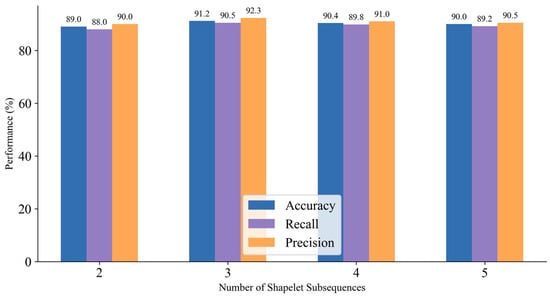
Figure 4. Performance Comparison for Different Numbers of Shapelet Subsequences.

As the number of shapelets increases from 2 to 3, all three metrics—accuracy, recall, and precision—show noticeable improvements. This suggests that adding a third shapelet helps capture more comprehensive and discriminative time-series patterns. However, when the number increases further to 4 and 5, performance slightly declined. This is likely due to the introduction of less informative or redundant subsequences, which can increase model complexity and risk of overfitting. Using 3 shapelets yields the highest performance with 91.2% accuracy, 90.5% recall, and 92.3% precision. This configuration effectively balances representational power and feature compactness, enabling the model to learn key patterns without being overwhelmed by irrelevant information. The model achieves a favorable balance between detecting true positives and avoiding false alarms. This is especially valuable in safety-critical domains such as lost circulation monitoring, where both sensitivity and reliability are essential.

From a deployment perspective, using 3 shapelets also keeps feature dimensionality low, reducing computational cost during real-time prediction. This makes it well-suited for integration into field-deployable monitoring systems. With three well-selected shapelets, the model is better able to recognize subtle and early-stage changes in the time series, such as gradual pressure increases or slight gas flow anomalies. This allows for earlier warning signals, providing critical time for intervention and preventive measures.

These results demonstrate that the number of shapelets has a direct impact on classification performance. In this study, three shapelets provided the best trade-off between accuracy, efficiency, and early detection. The findings offer valuable guidance for tuning shapelet-based models in real-world time series risk monitoring applications.

3.4. Real-Time Model Updating

In real-world drilling operations, environmental conditions, geological formations, and sensor behaviors can change dynamically over time. To address this, we explored whether allowing the model to perform real-time updates during the prediction phase could improve its adaptability and predictive performance. This approach simulates online learning, where the model incrementally incorporates newly labeled samples during the monitoring process.

Using the previously optimized SVM model with shapelet transformation, we compared two settings:

Static model: The model is trained once offline and then used for prediction without further updates. In this baseline setting, the SVM is trained once on the training set, and its parameters remain unchanged during all subsequent predictions.

Online-updated model: After each batch of incoming time-series data, a small portion of samples with the highest prediction confidence (top 5%) is used to incrementally update the classifier, mimicking how drilling data accumulate in real operations. A confidence threshold of 0.95 is applied, and the model is updated at most once per batch using no more than ten newly collected samples. During each cycle, samples whose predicted probabilities exceed the threshold are temporarily stored, and a lightweight parameter update is performed at the end of the batch before the buffer is cleared. This controlled update process enables the model to gradually adapt to evolving drilling conditions while reducing the risk of reinforcing misclassified patterns, thereby maintaining stable predictive behavior over time.

Both settings were evaluated on the same test dataset to ensure fairness. The online update was performed using a limited learning rate and capped update frequency to avoid catastrophic forgetting.

As shown in Figure 5, the experimental results clearly indicate that the real-time updated model outperforms the static model across all three key performance metrics: accuracy, recall, and precision. Accuracy improved from 91.2% to 93.1%, recall increased from 90.5% to 92.8%, and precision rose from 92.3% to 93.7%. This consistent upward trend demonstrates that the online updating mechanism enables the model to adapt to evolving data distributions over time and enhances its responsiveness to newly emerging or subtle risk patterns—especially under complex downhole conditions where data characteristics may gradually shift. Notably, the improvement in precision also implies a reduction in false positives, which is highly valuable in operational settings for reducing false alarms, minimizing unnecessary shutdowns, and lowering overall costs. Compared to conventional static models that often overfit outdated patterns, the real-time updated model exhibits a form of self-calibration, maintaining robustness and adaptability throughout the monitoring process.

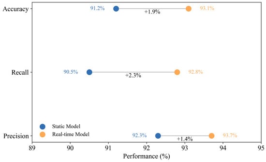
Figure 5. Performance Comparison Between Static and Real-Time Updated Models.

Furthermore, the update mechanism is designed with safeguards: only high-confidence predictions are used for incremental updates, and a low learning rate is employed to prevent instability. This conservative strategy ensures that the model learns efficiently from new data while avoiding performance degradation due to noisy or anomalous inputs. The findings confirm that the shapelet-based model is scalable and reliable under dynamic conditions, offering a solid technical foundation for deploying intelligent lost circulation monitoring systems in real-time operational environments.

4. Conclusions

In this study, we proposed a novel method for lost circulation risk monitoring based on time series shapelet transformation, data augmentation with RCGAN, and gradient boosting classifiers. The experimental results confirm the effectiveness of the proposed approach in enhancing predictive accuracy, early warning capability, and model robustness.

First, the use of RCGAN-based data augmentation significantly improved model performance during training by generating diverse and realistic synthetic samples. This process effectively mitigated the limitations posed by small and imbalanced datasets, enabling the model to better learn latent risk signals that are underrepresented in real-world drilling data. By filling information gaps, GANs helped improve the generalization ability of all models, especially in capturing rare lost circulation patterns.

Second, shapelet transformation proved to be a powerful technique for time series feature extraction. By converting raw sequences into discriminative subsequence-based features, the model could focus on key local patterns—such as subtle temporal fluctuations in drilling parameters or mud volume—that may serve as early indicators of lost circulation events. This not only reduced data dimensionality and computational complexity but also significantly improved classification accuracy, particularly for minority-class abnormal events.

Third, we conducted a comparative evaluation of several classifiers. The results showed that the tested models—SVM, kNN, LR, and ANN—exhibited distinct performance patterns, with SVM, kNN, and LR consistently achieving higher accuracy, recall, and precision than the Artificial Neural Network (ANN). Among them, SVM achieved the best overall results, with high accuracy, precision, and recall. These models required less data preprocessing and demonstrated greater stability on small to medium-sized datasets, making them well-suited for deployment in drilling environments.

Finally, the incorporation of a real-time model updating mechanism further enhanced the system’s adaptability and responsiveness. By incrementally updating the model with high-confidence predictions, the approach allowed for continuous learning and adjustment to new or evolving patterns in the data stream. This led to additional improvements in accuracy and recall and provided a pathway toward building intelligent, field-deployable lost circulation monitoring systems capable of adapting to dynamic drilling conditions.

In summary, the integration of RCGAN-based augmentation, shapelet-based time series transformation, gradient boosting classifiers, and real-time learning forms a comprehensive and effective framework for lost circulation risk monitoring. Future work may explore adaptive thresholding, uncertainty quantification, and hardware-oriented model optimization for real-time edge deployment in drilling control systems.

References

- Skogdalen, J.E.; Utne, I.B.; Vinnem, J.E. Developing safety indicators for preventing offshore oil and gas deepwater drilling blowouts. Saf. Sci. 2011, 49, 1187–1199. [Google Scholar] [CrossRef]
- Choubey, S.; Karmakar, G.P. Artificial intelligence techniques and their application in oil and gas industry. Artif. Intell. Rev. 2021, 54, 3665–3683. [Google Scholar] [CrossRef]
- Nan, C.; Khan, F.; Iqbal, M.T. Real-time fault diagnosis using knowledge-based expert system. Process Saf. Environ. 2008, 86, 55–71. [Google Scholar] [CrossRef]
- Al-Hameedi, A.T.; Alkinani, H.H.; Dunn-Norman, S.; Flori, R.E.; Hilgedick, S.A.; Amer, A.S.; Alsaba, M.T. Using machine learning to predict lost circulation in the Rumaila field, Iraq. In Proceedings of the SPE Asia Pacific Oil and Gas Conference and Exhibition, Brisbane, QLD, Australia, 23–25 October 2018; p. D031S027R003. [Google Scholar] [CrossRef]
- Geng, Z.; Wang, H.; Fan, M.; Lu, Y.; Nie, Z.; Ding, Y.; Chen, M. Predicting seismic-based risk of lost circulation using machine learning. J. Petrol. Sci. Eng. 2019, 176, 679–688. [Google Scholar] [CrossRef]
- Abbas, A.K.; Al-haideri, N.A.; Bashikh, A.A. Implementing artificial neural networks and support vector machines to predict lost circulation. Egypt J. Pet. 2019, 28, 339–347. [Google Scholar] [CrossRef]
- Hou, X.; Yang, J.; Yin, Q.; Liu, H.; Chen, H.; Zheng, J.; Wang, J.; Cao, B.; Zhao, X.; Hao, M. Lost circulation prediction in south China sea using machine learning and big data technology. In Proceedings of the Offshore Technology Conference, Houston, TX, USA, 4–7 May 2020; p. D041S053R005. [Google Scholar] [CrossRef]
- Shi, X.; Zhou, Y.; Zhao, Q.; Jiang, H.; Zhao, L.; Liu, Y.; Yang, G. A new method to detect influx and loss during drilling based on machine learning. In Proceedings of the International Petroleum Technology Conference, Beijing, China, 26–28 March 2019; p. D021S018R003. [Google Scholar] [CrossRef]
- Pang, H.; Meng, H.; Wang, H.; Fan, Y.; Nie, Z.; Jin, Y. Lost circulation prediction based on machine learning. J. Petrol. Sci. Eng. 2022, 208, 109364. [Google Scholar] [CrossRef]
- Sun, W.; Liu, K.; Zhang, D.; Li, W.; Xu, L.; Dai, Y. A kick and lost circulation monitoring method combining Bi-GRU and drilling conditions. Pet. Drill. Tech. 2023, 51, 37–44. [Google Scholar] [CrossRef]
- Wu, L.; Wang, X.; Zhang, Z.; Zhu, G.; Zhang, Q.; Dong, P.; Wang, J.; Zhu, Z. Intelligent Monitoring Model for Lost Circulation Based on Unsupervised Time Series Autoencoder. Processes 2024, 12, 1297. [Google Scholar] [CrossRef]
- Wu, S.; Hu, Y.; Zhang, L.; Liu, S.; Xie, R.; Yin, Z. Intelligent risk identification for drilling lost circulation incidents using data-driven machine learning. Reliab. Eng. Syst. Safe 2024, 252, 110407. [Google Scholar] [CrossRef]
- Benesty, J.; Chen, J.; Huang, Y.; Cohen, I. Pearson correlation coefficient. In Noise Reduction in Speech Processing; Springer: Berlin/Heidelberg, Germany, 2009; pp. 1–4. [Google Scholar] [CrossRef]
- Goodfellow, I.J.; Pouget-Abadie, J.; Mirza, M.; Xu, B.; Warde-Farley, D.; Ozair, S.; Courville, A.; Bengio, Y. Generative adversarial nets. Adv. Neural Inf. Process. Syst. 2014, 27, 1–9. [Google Scholar] [CrossRef]
- Zhou, D.; Zhou, C.; Zhang, Z.; Zhou, M.; Zhang, C.; Zhu, L.; Li, Q.; Wang, C. Intelligent Lost Circulation Monitoring Method Based on Data Augmentation and Temporal Models. Processes 2024, 12, 2184. [Google Scholar] [CrossRef]
- Sirisha, B.; Sandhya, B. Pressure sensor data modeling with recurrent conditional generative adversarial networks. In Proceedings of the 2022 9th International Conference on Computing for Sustainable Global Development (INDIACom), New Delhi, India, 23–25 March 2022; pp. 443–448. [Google Scholar] [CrossRef]
- Lines, J.; Davis, L.M.; Hills, J.; Bagnall, A. A shapelet transform for time series classification. In Proceedings of the 18th ACM SIGKDD International Conference on Knowledge Discovery and Data Mining 2012, Beijing, China, 12–16 August 2012; pp. 289–297. [Google Scholar] [CrossRef]
- Ye, L.; Keogh, E. Time series shapelets: A new primitive for data mining. In Proceedings of the 15th ACM SIGKDD International Conference on Knowledge Discovery and Data Mining 2009, Paris, France, 28 June–1 July 2009; pp. 947–956. [Google Scholar] [CrossRef]
- Hearst, M.A.; Dumais, S.T.; Osuna, E.; Platt, J.; Scholkopf, B. Support vector machines. IEEE Intell. Syst. Their Appl. 1998, 13, 18–28. [Google Scholar] [CrossRef]
- Peterson, L.E. K-nearest neighbor. Scholarpedia 2009, 4, 1883. [Google Scholar] [CrossRef]
- LaValley, M.P. Logistic regression. Circulation 2008, 117, 2395–2399. [Google Scholar] [CrossRef] [PubMed]
- Walczak, S. Artificial neural networks. In Advanced Methodologies and Technologies in Artificial Intelligence, Computer Simulation, and Human-Computer Interaction; IGI Global Scientific Publishing: Hershey, PA, USA, 2019; pp. 40–53. [Google Scholar] [CrossRef]
- Khormali, A.; Ahmadi, S.; Aleksandrov, A.N. Analysis of reservoir rock permeability changes due to solid precipitation during waterflooding using artificial neural network. J. Pet. Explor. Prod. Technol. 2025, 15, 17. [Google Scholar] [CrossRef]
- Chen, T.; Guestrin, C. Xgboost: A scalable tree boosting system. In Proceedings of the 22nd ACM SIGKDD International Conference on Knowledge Discovery and Data Mining 2016, San Francisco, CA, USA, 13–17 August 2016; pp. 785–794. [Google Scholar] [CrossRef]
Disclaimer/Publisher’s Note: The statements, opinions and data contained in all publications are solely those of the individual author(s) and contributor(s) and not of MDPI and/or the editor(s). MDPI and/or the editor(s) disclaim responsibility for any injury to people or property resulting from any ideas, methods, instructions or products referred to in the content. |
© 2025 by the authors. Licensee MDPI, Basel, Switzerland. This article is an open access article distributed under the terms and conditions of the Creative Commons Attribution (CC BY) license (https://creativecommons.org/licenses/by/4.0/).