Abstract
Deep to ultra-deep carbonate formations have become crucial targets for oil and gas exploration. However, owing to the low accuracy of carbonate formation pressure prediction during drilling, complex incidents such as collapse, block shedding, and drilling fluid loss frequently occur, severely restricting the efficient development of deep and ultra-deep oil and gas resources. This study targets the Tarim Basin, integrating well-logging and geological data from six wells, with depths ranging from 5000 to 9000 m, through multi-source data fusion. These results indicate that abnormal overpressure in the carbonate formations is chiefly governed by hydrocarbon generation and tectonic compression. Accordingly, 10 key characteristic parameters related to the cause of over-pressure were identified. The Support Vector Regression (SVR) model and Long Short-Term Memory (LSTM) neural network model were used to predict the pressure of carbonate rock formations. The constructed LSTM model demonstrated better prediction results for formation pressure than the SVR model. Compared with the traditional Bowers effective stress method, the LSTM model achieves an exact mean relative error range of 0.256–3.846% for a single well, which is significantly lower than the prediction accuracy of the Bowers effective stress method. The study shows that the LSTM machine learning algorithm can more accurately predict the formation pressure distribution characteristics of the carbonate formations in the research area. This provides reliable foundational data support for safe drilling in the carbonate rock formations of the Tarim Basin and offers valuable insights for pressure prediction in similar regions.
1. Introduction
Deep and ultra-deep carbonate rock formations contain very rich oil and gas resources. During the exploration and development process, accurate evaluation of the formation pressure is crucial for determining drilling fluid density, designing the wellbore structure, and planning well networks. It is one of the key technologies to ensure the smooth progress of exploration and development. In deep carbonate formations of the Tarim Basin, frequent wellbore instability, loss of circulation, and collapse incidents occur due to inaccurate formation pressure prediction, which seriously restricts the safe and efficient drilling process. Before drilling begins, people predict the formation pressure using logging data or seismic data from neighboring well blocks for inversion analysis. Common traditional formation pressure prediction methods include the Eaton method [1], effective stress method [2], Bowers method [3], Fillippone method [4], and the equivalent depth method [5]. Unlike clastic undercompaction, carbonate overpressure arises from fracture-dominated pore systems and diagenetic modification rather than compaction-driven porosity retention [6]. It is necessary to construct corresponding models for formation pressure prediction based on the cause mechanism of the formation pressure. The underlying mechanism of abnormal pressure in carbonate rocks differs from the under-compaction effect in conventional sandstone and mudstone. After conducting a comprehensive analysis of the cause mechanism of abnormal pressure in carbonate rocks, the formation pressure of carbonate rock formations can be predicted. Abdelaal et al. [7] predicted the formation pressure of carbonate rock fractured-porous reservoirs based on the theory of the equivalent depth method. Xia et al. [8] used the effective stress method, performed multiple linear regressions between effective stress, the ratio of compressional and shear wave velocities, and Poisson’s ratio to obtain a calculation method for the formation pressure of carbonate rock formations in northeastern Sichuan. Zhao et al. [9] addressed the strong heterogeneity and complex cause mechanisms of abnormal pressure in fracture-cave-type carbonate rocks, separately established formation pressure prediction models using the equivalent depth method, the Eaton method, and the effective stress method. This approach avoids issues of low accuracy and large errors caused by single factors, meeting the prediction requirements for formation pressure in fracture-cave-type carbonate rock formations.
Traditional approaches rely heavily on the correction of certain parameters using measured data points or offset-well information, or require calibration through core testing to improve prediction accuracy. Consequently, these methods exhibit substantial limitations in practical applications. With the continuous advancement of science and technology, machine learning algorithms have been increasingly applied in hydrocarbon exploration. By training machine learning models, it becomes possible to achieve more accurate and reliable predictions of formation pressure [7,10,11,12]. For the problem of formation pressure prediction, the most suitable and widely applied machine learning algorithms are support vector machines (SVMs) and neural networks. Among neural network models, the most commonly employed include artificial neural networks (ANN), long short-term memory networks (LSTM), convolutional neural networks (CNN), and back-propagation neural networks (BP). Dong et al. [13] developed a formation pressure prediction model for fractured carbonate reservoirs using the BP algorithm by incorporating four key factors controlling pressure evolution. Keshavarzi [14] integrated the backpropagation neural network (BP) algorithm with the generalized regression neural network to establish a formation pressure prediction model. Bungasalu [15] applied a hybrid model that combines the Eaton method with artificial neural networks (ANN) for complex carbonate oilfields, which significantly improved the accuracy of formation pressure prediction. Farsi [16] employed a hybrid approach integrating multiple intelligent algorithms with particle swarm optimization (PSO) to predict formation pressure in the Marun oilfield, Iran, achieving satisfactory performance in field applications. Khaled [17] proposed the use of artificial neural networks (ANN) to predict fractures and formation pressure during drilling in mixed lithologies. Xu et al. [18] proposed a formation pressure prediction method based on a combined convolutional neural network and long short-term memory network (CNN-LSTM) model. Recent studies have shown that incorporating various industrial wastes—such as marble powder, ceramic powder, and waste fire clay—can enhance concrete performance while enabling reliable strength prediction through experimental and data-driven modeling approaches [19,20,21]. Machine learning algorithms effectively capture nonlinear relationships and enhance the generalization of pressure prediction models. Previous studies showed that these methods reduce prediction errors by approximately 20–40% compared with traditional empirical methods, demonstrating clear advantages in complex carbonate formations. Existing studies often rely on single-source data and limited feature selection; in contrast, our work leverages multi-source data fusion with mechanism-guided feature selection to enhance both prediction accuracy and interpretability.
Although machine learning algorithms can overcome some limitations of traditional methods, such as the dependence on core samples and specific datasets, the performance of machine learning models still relies heavily on the proper selection of input features. Inappropriate feature selection or insufficient understanding of geological mechanisms may lead to model overfitting or unreliable predictions. Since abnormal pressure mechanisms vary, selecting appropriate feature parameters is essential to ensure the reliability of prediction accuracy. Taking the ultra-deep carbonate formations of the Tarim Basin as an example, this study integrates multiple types of data to clarify the mechanisms of abnormal pressure in carbonate formations. By combining traditional formation pressure prediction methods with machine learning algorithms, the study investigates the distribution patterns of formation pressure in carbonate formations. This approach provides more accurate and reliable data for oil and gas exploration and development in ultra-deep carbonate reservoirs.
2. Mechanisms of Abnormal Pressure in Carbonate Formations
In the Tarim Basin, drilling in carbonate formations often results in severe circulation losses and collapse events, with over 30% of wells experiencing instability due to inaccurate pore pressure prediction. At present, the primary mechanisms responsible for abnormal overpressure in carbonate formations include fluid expansion, undercompaction, dissolution of formation rocks, and tectonic compression [22,23,24]. The identification methods for abnormal pressure mechanisms can generally be categorized into two groups: (1) log-based approaches, which rely on variations in petrophysical parameters reflected in well logging data; (2) geological approaches, which determine the mechanisms of abnormal pressure through analyses of source rock thermal maturity and regional tectonic evolution [25,26,27].
2.1. Integrated Analysis of Well Logging Data
Well logging curves directly reflect lithology, physical properties, and hydrocarbon-bearing characteristics, providing an important theoretical basis for oil and gas exploration and development. Combined analysis of multiple logging curves enables a more comprehensive and accurate interpretation of formation characteristics.
- (1)
- Acoustic velocity–density method
The crossplot method of acoustic velocity and density, established based on the theory of Bowers, is a commonly used approach for rock physics analysis and reservoir overpressure evaluation. By utilizing the relationship between P-wave velocity and rock density, abnormal pressure detection can be achieved. The presence of overpressure can be identified by analyzing the variation trends of acoustic velocity–density scatter clusters in different formations.
In the above equation, vp denotes the P-wave velocity, m/s; a and b are fitting constants; and represents the density at a given depth, g/cm3.
In a normal pressure system, the P-wave velocity increases with depth, and the scatter plot of the acoustic velocity versus density is expected to be uniformly distributed along the normal compaction trend. Under undercompaction conditions, the formation density decreases and the corresponding P-wave velocity decreases. If fluid expansion occurs, the relationship between acoustic velocity and density deviates from the original trend since the formation density may continue to increase while the P-wave velocity decreases [28]. When tectonic compression takes place, both formation density and P-wave velocity increase; however, the scatter points of acoustic velocity and density still deviate from the normal trend line, as shown in Figure 1a.
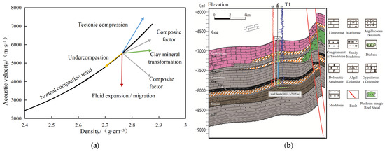
Figure 1.
Logging responses of geological characterization: (a). acoustic velocity–density relationships under geological processes; (b) depth–lithology profile of T1.
The Tarim Basin, located in northwest China, features extensive ultra-deep carbonate reservoirs with complex structures and diverse stratigraphy, making it a suitable site for overpressure studies. Taking Well T1 in the Tarim Basin as an example, an acoustic velocity–density crossplot was constructed using the normal compaction trend of sandstone and mudstone formations, with the complete stratigraphic coverage and high-quality logging data enabling robust evaluation of predictive models. The lithological distribution corresponding to these depths is shown in Figure 1b. The analysis encompasses carbonate formations from four stratigraphic intervals, namely the Carboniferous, Ordovician, Cambrian, and Sinian strata, with depth increasing progressively.
As shown in Figure 2a, the scatter points of the Carboniferous data are distributed uniformly along the normal compaction trend line, indicating a normally compacted formation. In contrast, the scatter points corresponding to the Ordovician–Sinian intervals exhibit systematically elevated density and acoustic velocity values, deviating markedly from the normal compaction trend. This systematic deviation is interpreted as evidence of tectonic compression acting on these formations.
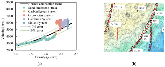
Figure 2.
Abnormal pressure detection: (a) crossplot of acoustic velocity and density; (b) structure diagram of the top layer.
- (2)
- Acoustic velocity–vertical effective stress method
When the formation is normally compacted, the relationship between vertical effective stress and compressional wave velocity follows an exponential trend, which is referred to as the normal compaction trend (NCT) or the virgin loading curve, as shown in Figure 3. The curves represent typical stress–acoustic velocity trends, illustrating the general behavior of rock under loading and unloading rather than specific experimental measurements.
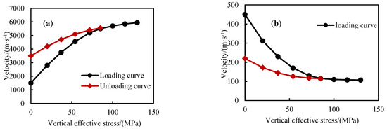
Figure 3.
Typical stress–acoustic velocity curves: (a) loading curve; (b) unloading curve.
When the effective stress acting on the rock decreases, pore spaces may recover, resulting in a reduction in acoustic velocity, which is consistent with the unloading curve behavior. As illustrated in the figure, in undercompacted formations, the relationship between velocity and vertical effective stress generally follows a linear or exponential trend, whereas formations affected by fluid expansion, overpressure transmission, or lateral tectonic compression deviate from the normal compaction trend line [29]. The mathematical relationship can be formulated as follows:
where represents the vertical effective stress at a given depth, MPa. The loading curve corresponding to abnormal overpressure is consistent with the undercompaction theory proposed by Bowers. Overpressure induced by tectonic compression leads to an increase in acoustic velocity, while the vertical effective stress decreases or remains unchanged. In contrast, overpressure caused by fluid expansion results in a reduction in vertical effective stress with little variation in acoustic velocity. Both tectonic compression and fluid expansion-related overpressure correspond to the characteristics of the unloading curve. Taking Well T1 in the Tarim Basin as an example, the vertical effective stress was first calculated using the Bowers effective stress method, and the relationship between acoustic velocity and vertical effective stress was established to derive the normal compaction trend line.
As shown in Figure 4, the scatter points of the Carboniferous formation are evenly distributed along the normal compaction trend line, indicating normally compacted strata. In contrast, the Ordovician to Sinian formations deviate from the normal compaction trend line, and the vertical effective stress exhibits little variation as the acoustic velocity decreases. These findings suggest that the carbonate strata of the Ordovician to Sinian intervals may have developed abnormal overpressure due to the combined effects of fluid expansion and tectonic compression.

Figure 4.
Crossplot of the acoustic velocity and vertical effective stress.
Through an integrated analysis of the P-wave velocity–density crossplot and P-wave velocity–vertical effective stress crossplot of carbonate formations in the Tarim Basin, the following preliminary conclusions can be drawn: the Carboniferous formation exhibits normal compaction characteristics, whereas the Ordovician, Cambrian, and Sinian formations are likely influenced by tectonic compression and fluid expansion, resulting in the development of abnormal overpressure.
2.2. Comprehensive Analysis of Abnormal Pressure Based on Geological Data
The presence of hydrocarbon generation overpressure in carbonate formations can be evaluated based on the maturity of source rocks and related geochemical indicators. Total organic carbon (TOC), maximum pyrolysis temperature (Tmax), vitrinite reflectance (RO), hydrocarbon generation potential (S1 + S2), and chloride ion content are the primary parameters controlling hydrocarbon generation. In general, when Ro exceeds 0.5 (the hydrocarbon generation threshold) and Tmax is greater than 435 °C, the source rock enters the mature stage and is capable of generating large volumes of oil and gas. Hydrocarbon generation potential (S1 + S2) provides insight into the maximum capacity of source rocks to generate hydrocarbons (oil and natural gas) during pyrolysis, whereas higher chloride ion content favors the preservation of organic matter and promotes hydrocarbon generation. In addition, the crossplot of methane, ethane, and propane can be employed to further verify the occurrence of hydrocarbon generation processes. A systematic interpretation of each of these controlling factors is presented below.
- (1)
- Vitrinite Reflectance (RO)
Based on the vitrinite reflectance (RO) data of the Ordovician to Sinian formations in the Tarim Basin (Figure 5), the source rocks of the Lower Cambrian Yurtus Formation exhibit a progressive increase in RO from the Caledonian, Hercynian, and Yanshanian periods to the present. This trend reflects the long-term thermal evolution of the source rocks. Specifically, during the Caledonian period, RO values were relatively low, indicating an early stage of thermal evolution in which organic matter had not yet reached the threshold for significant hydrocarbon generation. In the Hercynian period, particularly in the late Hercynian, tectonic activity and magmatism enhanced the thermal maturity, resulting in a marked increase in RO and driving the source rocks into the peak hydrocarbon generation stage. Subsequently, during the Yanshanian–Himalayan periods, thermal evolution further intensified, and certain intervals reached a high-maturity stage. At present, the vitrinite reflectance of the Yurtus Formation exceeds 1.8%, indicating an over-mature stage and confirming its status as a high-quality source rock.
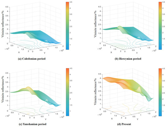
Figure 5.
Hydrocarbon generation and expulsion history of Cambrian source rocks: (a) Caledonian period. (b) Hercynian period. (c) Yanshanian period. (d) Present.
- (2)
- Maximum pyrolysis temperature (Tmax), total organic carbon (TOC), and hydrocarbon generation potential (S1 + S2)
Taking Well T1 in the Tarim Basin as an example, the relationships among maximum pyrolysis temperature (Tmax), total organic carbon content (TOC), and hydrocarbon generation potential (S1 + S2) with depth were plotted based on 46 samples. The following conclusions can be drawn from Figure 6: in strata deeper than 8000 m, TOC consistently exceeds the hydrocarbon generation threshold, with values greater than 0.5%, while Tmax exceeds 430 °C. This indicates that the strata within this depth interval have already entered the hydrocarbon generation window and possess considerable hydrocarbon generation potential.
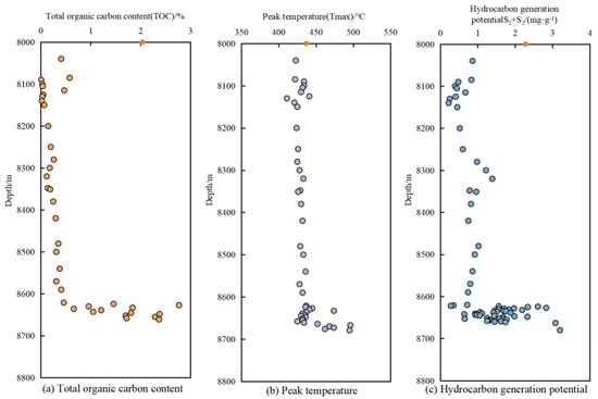
Figure 6.
Relationships between total organic carbon content, peak temperature, and hydrocarbon generation potential, and depth of Cambrian source rocks (orange points indicate median values).
Notably, at depths of 8600–8700 m, both organic matter abundance and thermal maturity markedly increased. TOC reaches as high as 3%, far above the hydrocarbon threshold, indicating significant organic matter enrichment that provides a robust material basis for hydrocarbon generation. Meanwhile, Tmax rises to 500 °C, suggesting that the strata have experienced intense thermal evolution, with organic matter entering a highly mature stage characterized by strong hydrocarbon generation capacity.
In terms of hydrocarbon generation potential (S1 + S2), this interval presents markedly higher values than other depth ranges, further confirming favorable hydrocarbon generation conditions. By integrating TOC and Tmax data, it can be inferred that this depth interval not only contains abundant organic matter but also exhibits suitable thermal maturity, thereby constituting a key horizon for deep hydrocarbon generation.
- (3)
- Chloride ion content
Chloride ion content indirectly influences hydrocarbon generation by affecting organic matter preservation, thermal maturation, hydrocarbon migration, and the depositional environment. Taking Well T1 in the Tarim Basin as an example (Figure 7), chloride concentrations range between 8000 and 180,000 mg/L, generally exhibiting an increasing trend with depth. This variation is consistent with the sedimentary evolution and formation water characteristics of the basin. In shallow intervals, the relatively low chloride concentrations are primarily attributed to dilution by meteoric water, whereas in deeper intervals, the significantly elevated chloride contents reflect a more enclosed geochemical environment that favors organic matter preservation and hydrocarbon generation. Chloride ion content reflects paleo-salinity and fluid retention; higher salinity favors organic matter preservation and is often associated with deeper, more thermally mature intervals.
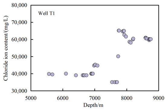
Figure 7.
Relationship between chloride ion content and depth in carbonate formations in the Tarim Basin.
Specifically, in Well T1, chloride concentration markedly increased between 5500 and 8900 m, with a particularly sharp rise in the 7500–8900 m interval. This increase corresponds well with the depth intervals characterized by elevated total organic carbon (TOC) and maximum pyrolysis temperature (Tmax), suggesting that higher chloride concentrations may increase the hydrocarbon generation potential by improving organic matter preservation and facilitating thermal maturation. Similar trends are observed in other wells, particularly in deeper source rocks, where increasing chloride concentrations exhibit a positive correlation with hydrocarbon generation potential.
- (4)
- Methane, ethane, and propane (C1, C2, and C3)
Based on the data from Well T1 in the Tarim Basin, methane (C1), ethane (C2), and propane (C3) were selected to construct a cross-plot of Ln(C1/C2) versus Ln(C2/C3) (Figure 8). This plot is commonly used to distinguish between kerogen cracking gas and oil cracking gas, thereby providing indirect evidence for the occurrence of hydrocarbon generation.
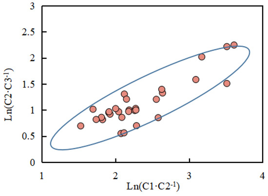
Figure 8.
Diagram of Ln(C1/C2) and Ln(C2/C3) in carbonate rocks in the Tarim Basin.
The values of Ln(C1/C2) and Ln(C2/C3) for Well T1 exhibit a wide distribution range. Specifically, Ln(C1/C2) varies from 1.527 to 3.612, and Ln(C2/C3) ranges from 0.548 to 2.244. In general, Ln(C1/C2) spans a broader interval (0.883–6.013) than Ln(C2/C3) (0.147–3.156), indicating that the natural gas in the carbonate formations of Well T1 is predominantly derived from kerogen cracking, with potential contributions from oil cracking gas in certain intervals.
The slope of the Ln(C1/C2) versus Ln(C2/C3) plot is less than 1, indicating the predominance of kerogen cracking gas. High Ln(C1/C2) values suggest that the natural gas has experienced a relatively high degree of thermal maturity, consistent with the high maturity characteristics of deep source rocks in the Tarim Basin. The broader distribution of Ln(C2/C3) values may reflect variations in the thermal maturity and organic matter types of source rocks at different depths. Overall, the compositional characteristics of natural gas indicate the dominance of kerogen cracking gas, further confirming the significant hydrocarbon generation processes in the study area.
2.3. Tectonic Compression
During the Caledonian period, the Tarim block transitioned from oceanic basin expansion to closure and compression, leading to the initial development of the Tabei uplift and the Lunnan low uplift. The southwest–northeast-oriented compressive stress during this stage resulted in the preliminary uplift and deformation of strata. The formation of a marine carbonate paleouplift in the Tabei area provided a structural foundation for subsequent overpressure development.
In the early Hercynian, the northern and central Tarim Basin were subjected to north–south-directed compressive stress, and the Lunnan low uplift gradually evolved into a southwestward-dipping nose-shaped uplift during the uplift process. By the late Hercynian, intense compressive tectonism induced folding and faulting, reducing rock pore volume and increasing the fluid pressure. The near east–west fold and fault systems generated during this stage created critical conditions for the development of overpressure.
During the Himalayan orogeny, compressional stress in the Tarim Basin further intensified, resulting in pronounced folding and faulting, further reduction in pore volume, and significant increases in fluid pressure. In addition, tectonic activity caused uplift and erosion along the basin margins, while maintaining sealing conditions within the basin, thereby amplifying overpressure generation. The multiphase tectonic movements in the basin formed fault systems that penetrated the Cambrian source rocks, serving as migration pathways for hydrocarbons and conduits for pressure transmission. The Xiaorbulake and Yurtus formations, composed of dense limestones with high mud content and poorly developed fractures, acted as effective caprocks. A structural map of the top of the formation is provided to illustrate regional tectonic features and deformation patterns(Figure 2b). Consequently, tectonic compression is considered one of the key mechanisms responsible for the development of abnormal overpressure in the Tarim Basin carbonates.
2.4. Drilling Parameter Responses to Hydrocarbon Generation and Tectonic Compression
Due to hydrocarbon generation, the diagnostic responses of the drilling parameters to hydrocarbon generation are shown in Table 1. The synergistic variations in these parameters can serve as effective indicators for identifying hydrocarbon-related overpressure intervals. In contrast, the response characteristics of drilling parameters influenced by tectonic compression are shown in Table 2.

Table 1.
Response characteristics of hydrocarbon generation to drilling parameters.
Table 2.
Response characteristics of tectonic compression to drilling parameters.
The presence of hydrocarbon gases in the drilling fluid affects multiple drilling and logging parameters. Gas entry causes volumetric expansion, leading to a decrease in outlet fluid density, while the associated heat absorption reduces the fluid outlet temperature. Concurrently, gas displacement accelerates the decline in outlet conductivity, lowering the inlet-to-outlet conductivity ratio. In terms of gas logging, hydrocarbon enrichment increases the total hydrocarbon content, with methane concentration rising rapidly; in highly mature carbonate formations, methane constitutes the dominant fraction of hydrocarbon gases. Meanwhile, well logging parameters reflect the increase in pore fluid pressure induced by hydrocarbons, manifested as a gradual rise in acoustic transit time. This effect is less pronounced in dolomite compared to limestone due to the lower sensitivity of the acoustic response to pressure variations. Additionally, the low electrical conductivity of hydrocarbons results in a significant decrease in formation resistivity.
Tectonic compression influences drilling fluid, gas logging, and well logging parameters by modifying fracture systems and rock properties. Increased compressive stress can either enhance or reduce the inlet–outlet density difference in drilling fluid, depending on the balance between fracture opening and compaction, while outlet conductivity fluctuates due to fluid exchange within fractures, often increasing in limestone intervals. Outlet temperature generally remains stable, though friction along fractures may cause abrupt spikes. Gas logging parameters, including total hydrocarbons and methane, typically show minimal variation under compression; however, if tectonic stress promotes connectivity with deeper reservoirs, sudden hydrocarbon enrichment may occur, particularly in limestone formations. Well logging responses reflect rock compaction, with acoustic transit time decreasing more markedly in limestone compared to other lithologies. Resistivity tends to increase due to reduced porosity, whereas negative anomalies in spontaneous potential are commonly associated with compressional zones.
3. Formation Pressure Prediction Using the Bowers Effective Stress Method
Based on the above abnormal pressure mechanism in the Tarim Basin, where overpressured formations are formed by hydrocarbon generation and tectonic compression, the unloading curve equation of the Bowers effective stress method is applicable. Therefore, the Bowers effective stress method is selected for formation pressure prediction in the study area.
The Bowers effective stress method establishes the original loading curve (shown in Figure 3) by using the relationship between compressional wave velocity and effective stress for normally compacted formations, without relying on traditional normal trend lines. This method uses deviations between measured data and the loading curve to identify the cause of abnormal pressure: formations with abnormally high pressure that conform to the under-compaction theory belong to the extended section of the loading curve, while abnormally high-pressure formations formed by fluid expansion and tectonic compression belong to the unloading curve characteristics. The relevant equations are shown in Equations (3) and (4).
where vpn denotes the fitted acoustic velocity, m/s; v0 is the acoustic velocity at zero effective stress, m/s; X and Y are the fitting coefficients of the curve model; represents the vertical effective stress at the onset of unloading, MPa; vi is the acoustic velocity at the onset of unloading, m/s; and U is the elasto-plastic coefficient, dimensionless.
By applying the loading and unloading curve equations, the vertical effective stress can be directly calculated. Subsequently, based on the effective stress principle, the formation pressure (pp) is determined from the overburden pressure(po) and the vertical effective stress, expressed as follows:
4. Formation Pressure Prediction Method Based on Machine Learning
Considering the overpressure mechanisms and strong heterogeneity of carbonate formations in the Tarim Basin, this study selects two typical machine learning models for formation pressure prediction: Support Vector Regression (SVR), which ensures prediction stability through structural risk minimization, and Long Short-Term Memory (LSTM) networks, which effectively capture the dynamic evolution of parameters.
4.1. Support Vector Regression (SVR)
The core idea of Support Vector Regression is to find an optimal hyperplane such that most data points fall within a defined margin while minimizing the prediction error.
The objective of SVR is to determine a regression function such that the majority of data points fall within a predefined tolerance margin ε. Data points located inside the ε-tube are not penalized, whereas those outside the tube are assigned a loss proportional to their distance from the boundary. To maximize the margin, SVR is formulated to minimize . In order to accommodate data points lying outside the ε-tube and to balance model complexity with training error, slack variables and a penalty parameter C are introduced. Accordingly, the optimization objective of SVR is formulated as shown in Equation (8).
In the calculation process, the objective is to ensure that most data points fall within the ε-insensitive tube while allowing a portion of the data points to lie outside the tube. Accordingly, the following constraints are imposed on the data points as expressed:
4.2. Long Short-Term Memory Neural Network (LSTM)
The Long Short-Term Memory (LSTM) neural network, as a special type of Recurrent Neural Network (RNN), captures the temporal variation patterns of formation pressure primarily through a gating mechanism. It mainly consists of an input gate, a forget gate, an output gate, and a memory cell state, as illustrated in Figure 9.
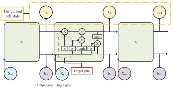
Figure 9.
LSTM model structure [30].
- (1)
- Memory cell and input gate: The memory cell serves as the core of the LSTM, responsible for storing and transmitting long-term information. The input gate determines which new information is allowed to enter the memory cell.
In the above equation, represents the output of the input gate, and denotes the sigmoid activation function. Wi and bi are the weight matrix and bias vector of the input gate, respectively. ht−1 is the hidden state at the previous time step, while xt is the current input. Ct1 denotes the candidate cell state, with Wc and bc being its corresponding weight matrix and bias vector, respectively.
- (2)
- Forget gate: This determines which information should be discarded from the cell state.
In the above equation, ft denotes the output of the forget gate, while Wf and bf represent the weight matrix and bias vector of the forget gate, respectively.
- (3)
- Cell state update: The cell state is updated based on the combined regulation of the forget gate and the input gate.
In the above equation, Ct and Ct−1 represent the cell states at time step t and t − 1, respectively.
- (4)
- Output gate: Determines which information from the memory cell is transferred to the output.
4.3. Data Preparation and Processing
4.3.1. Data Preparation
In the study area, the overpressure mechanism is primarily controlled by tectonic compression and hydrocarbon generation, both of which jointly affect the distribution of formation pressure. The data utilized in this study mainly consist of well logging data, drilling fluid data, and gas logging data. Based on the overpressure mechanisms and the response characteristics of the drilling parameters, the main influencing factors can be categorized into two groups, as shown in Table 3.
Table 3.
Influencing factors of overpressure causes.
4.3.2. Data Processing
Logging data were sampled every 1 m along the well depth, and both single-well and multi-well datasets were constructed. Cross-validation and early stopping were applied to the LSTM model to ensure generalization. Due to the complex geological conditions of the Tarim Basin and the frequent occurrence of complications, numerous outliers and missing values often appear during well logging. These data anomalies can introduce significant errors in formation pressure prediction. Therefore, data preprocessing of the raw dataset is required before conducting formation pressure prediction.
For certain missing values in the dataset, the linear interpolation method is applied for imputation. The specific steps include data sorting, missing value identification, linear interpolation, and boundary treatment. The logging data are sequentially sorted according to increasing well depth. If a missing value xi exists, it is marked as null. For two non-missing values xa (preceding value) and xb (subsequent value), the interpolation formula for xi is given by Equation (18). If the missing value occurs at the beginning or end of the sequence, it is filled with the first or last valid value, respectively. To evaluate the impact of interpolation, a sensitivity analysis was performed comparing predicted pressures with and without linear interpolation. The results indicate that the differences introduced by interpolation are negligible due to the high density of the logging data (1 m interval), confirming that linear interpolation does not significantly affect model accuracy.
In the above equation, a and b represent the indices before and after the missing point, respectively, and i represents the index of the missing point.
For outliers in the dataset, the K-means clustering algorithm is applied for anomaly detection. First, the data are clustered by specifying the number of clusters. Normal data values tend to cluster around the cluster centers, while outliers are located farther away from any center. Then, the distance of each data point to its corresponding cluster center is calculated. Based on the distance distribution, the 80th percentile (80% of the data points have distances smaller than this value) is taken as the anomaly detection threshold. This threshold was chosen to balance sensitivity and robustness, capturing extreme deviations while retaining most representative data points. Data points with distances exceeding this threshold are identified as outliers. These outliers are subsequently replaced with the mean value to achieve anomaly correction. Taking the logging data from Well T1 as an example, the acoustic transit time and total hydrocarbon content were processed for outlier detection and replacement. As shown in Figure 10, the original outliers were smoothed, and the variation trend of the parameter curves became more reasonable.
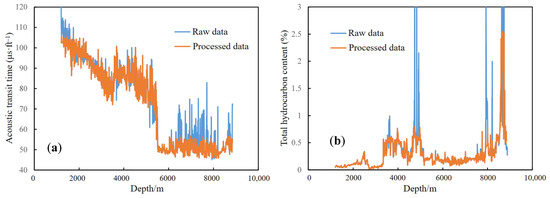
Figure 10.
Comparison of the data processing results in well T1: (a) acoustic velocity; (b) total hydrocarbon content.
The discrepancies caused by differences in data scale and units during the computation process of machine learning algorithms should be addressed. For example, the acoustic transit time may range from 40 to 140 μs/ft, while the total hydrocarbon content may range from 0 to 3. Standardization is applied to the data, as shown:
where x represents the feature value, represents the mean of the feature value, and represents the standard deviation of the feature value. To avoid data leakage, the standardization parameters are computed exclusively from the training set, and the same parameters are subsequently applied to the validation and test sets.
In formation pressure prediction, the performance of machine learning algorithms highly depends on the proper selection of input feature parameters. To accurately reflect the physical properties and pressure state of the formation, it is essential to first screen out parameters that are significantly correlated with formation pressure as model inputs.
Commonly used correlation analysis coefficients include Pearson and Spearman. The former is typically used to measure the linear correlation between two continuous variables, while the latter is used to measure the monotonic relationship between two variables. Since the formation of overpressure in carbonate formations is influenced by multiple geological factors, the relationships between these parameters and formation pressure may exhibit nonlinear or non-strictly linear characteristics. Therefore, the Spearman correlation coefficient was adopted to more comprehensively evaluate the associations between parameters and formation pressure.
A correlation coefficient greater than 0.7 generally indicates a strong correlation, while a value between 0.5 and 0.7 indicates a moderate correlation. Hence, parameters with correlation coefficients above 0.5 were selected as input data for the SVR and LSTM models, with formation pressure as the output.
Compared with the approaches of Li et al., the present study focuses on carbonate formations and employs a broader set of correlation-selected parameters to more effectively capture their pressure-sensitive characteristics [31,32]. A total of 14 parameters from Table 3 were selected for correlation analysis, and the correlation strength between each parameter and formation pressure was obtained. Based on the correlation strengths in Figure 11, 10 parameters were selected as input features: well depth, gamma ray, rock density, inlet density, outlet density, inlet temperature, outlet temperature, inlet conductivity, outlet conductivity, and total hydrocarbon content. To verify the stability of the selected 10 features, a brief ablation test comparing the Top-5, Top-8, Top-10, and Top-12 correlated features was conducted. The results show that the 10-feature set achieves the best overall performance and avoids redundancy, supporting its use in the final model.
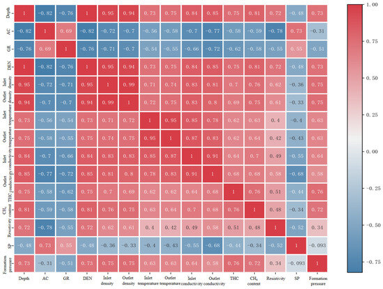
Figure 11.
Spearman correlation analysis.
To measure the generalization ability and optimization performance of the prediction models, four evaluation metrics were selected to analyze the accuracy of formation pressure prediction: Mean Absolute Error (MAE), Coefficient of Determination (R2), Mean Relative Error (MRE), and Mean Squared Error (MSE). R2 reflects the proportion of variance in the target variable explained by the model, with a range of (−∞, 1]. The closer R2 is to 1, the better the model fit. MAE represents the mean of the absolute errors between actual and predicted values, reflecting the actual error situation. MSE represents the mean of the squared errors between actual and predicted formation pressures. Accordingly, smaller MAE and MSE values indicate that the model predictions are closer to the actual values. MRE is expressed as a percentage, directly reflecting the error ratio.
The calculation formulas for the model evaluation metrics are as follows:
In the above equations, yi represents the actual formation pressure, and y′i represents the predicted formation pressure.
4.3.3. Comparison of Predictive Models
To establish a single-well model, the SVR and LSTM models were selected for single-well prediction of formation pressure. Due to the significant differences in algorithm principles and applicable conditions of the two models, the choice of hyperparameters directly affects the prediction accuracy and generalization ability. To ensure that the models can accurately reflect the distribution pattern of formation pressure in the study area, this section uses the logging and drilling fluid data from Well T1 to systematically train, test, and optimize the hyperparameters of the two models, in order to achieve the optimal prediction performance.
To avoid overfitting caused by the limited dataset, a 5-fold cross-validation strategy was adopted during model training. For the LSTM model, dropout regularization, early stopping, and validation-based hyperparameter tuning were applied to enhance model robustness and generalizability.
- (a)
- Establishment of the SVR model
The steps for using the SVR model for formation pressure prediction mainly include model initialization (data preparation, data processing, initialization of parameters, solving optimization, and obtaining regression parameters), model construction and evaluation (model training, testing, and evaluation), model optimization (test set and hyperparameter optimization), and result visualization. The flowchart is illustrated in the Figure 12.
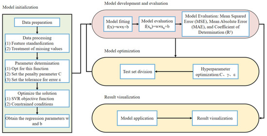
Figure 12.
Flowchart of formation pressure prediction by SVR model [33].
After data preprocessing, the number of input features for the SVR model was determined to be 11, and the output feature was 1. Initially, the test set ratio was set to 0.1 (i.e., the training set and test set were divided in a 9:1 ratio). Then, the regularization parameter C: [1, 10, 100, 500], the kernel parameter γ: [0.1, 0.5, 1, 5], and the width of the error tolerance band ε were initialized. The SVR model underwent grid search and cross-validation. The grid search exhaustively traverses all possible parameter combinations within the parameter space to identify the optimal solution. Based on the optimal parameter combination, the test set ratio was re-divided, and the model was retrained and tested to ensure that the training data were sufficient and the test results were reliable, as shown in Figure 13.
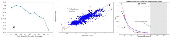
Figure 13.
The prediction results of the SVR model test set: (a) ratio of test set; (b) predicted results; (c) error values and training set.
In conclusion, the best prediction performance is achieved when the test set ratio is 0.2. For the SVR model, the evaluation metrics R2, MAE, and MSE were selected to optimize the parameter combination. As shown in Table 4 and Figure 14, when C remains unchanged and γ gradually increases, the evaluation metrics R2, MAE, and MSE show a gradually increasing trend, but after reaching the highest point, they begin to decrease. However, as C gradually increases, the γ value at the highest point gradually decreases.
Table 4.
Application effect of the SVR model on the test set.
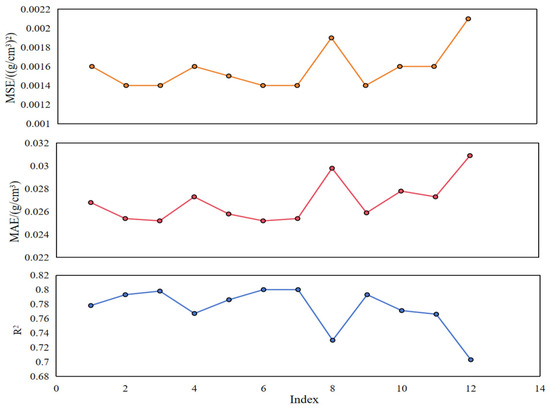
Figure 14.
Evaluation indicators of the SVR model.
During the parameter optimization process, by performing a grid search and cross-validation on the SVR model, it was found that when the parameter combination with serial number 6 was used for training and testing, the model exhibited the best overall performance. The evaluation metric R2 was the highest, indicating a good fit; MAE and MSE were the smallest, indicating the best model performance. Therefore, the SVR single-well model parameters were determined as follows: the test set ratio is 0.2, C is 10, γ is 0.5, and ε is 0.1. At this point, R2 is 0.8, MAE is 0.0252 g/cm3, and MSE is 0.0014 (g/cm3)2.
- (b)
- Establishment of LSTM model
The LSTM model has 11 input neurons and 1 output neuron. After data processing, model construction, and training, the model was tested, optimized, and evaluated. The process for predicting formation pressure using the LSTM model is shown in Figure 15.
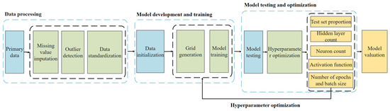
Figure 15.
Flowchart of formation pressure prediction by LSTM model.
The data from Well T1 were used for training, testing, and hyperparameter optimization. Initially, the test set ratio was set to 0.1 (i.e., the training set and test set were divided in a 9:1 ratio), and the model was trained and tested to find the optimal parameter combination. Based on the optimal parameter combination, the test set ratio was redivided, and the model was trained and tested again, as shown in Figure 16. The best prediction performance was achieved when the test set ratio was 0.2.
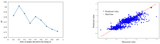
Figure 16.
Proportion and prediction results of the LSTM model test set.
The hyperparameters of the LSTM model mainly include the number of layers (excluding the input layer, ranging from [2, 3]), the number of neurons [32, 64], the activation function (relu), the number of epochs [100, 300], and the batch size [16, 32]. Model training was performed using the Adam optimizer combined with an early-stopping strategy, where training was terminated if the validation loss did not decrease for 30 consecutive epochs. The hyperparameters of the LSTM model were optimized, and the parameter combinations that performed well on the test set and the evaluation metrics are shown in Table 5 and Figure 17.
Table 5.
Application effect of LSTM model on the test set.
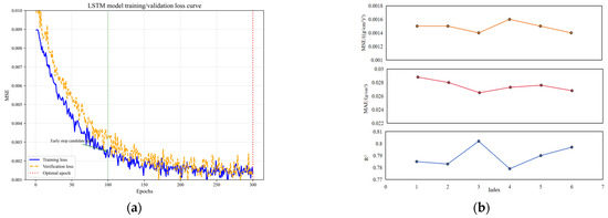
Figure 17.
Evaluation of LSTM model: (a) training loss of the model; (b) evaluation indicators.
Considering both the tables and figures, in terms of the coefficient of determination and mean absolute error, the model with serial number 3 performs the best; in terms of mean square error, the parameter combination at serial number 6 is the same as that at serial number 3. Considering three evaluation metrics, the model with the third parameter combination performs better. The LSTM model has two layers with 32 and 1 neurons, respectively, 300 epochs, and a batch size of 32. At this point, R2 is 0.802, MAE is 0.0265 g/cm3, and MSE is 0.0014 (g/cm3)2.
Analyzing multiple wells allows for more comprehensive characterization of formation pressure variations and improves the generalizability of the predictive models. By collecting relevant data from well T1, the SVR and LSTM models were trained and tested for multiple wells, and hyperparameter optimization was carried out.
- (a)
- Establishment of the SVR Model
The input features for the SVR model are 11, and the output feature is 1. After fixing the test set ratio at 0.1, the model was trained and tested. Hyperparameters of the SVR model were optimized, and after determining the optimal parameter combination, the test set ratio was redivided, as shown in Figure 18. The model performs best when the test set ratio is 0.1. The parameter combination that performs well on the test set is shown in Table 6, and the evaluation metric change diagram is shown in Figure 19.
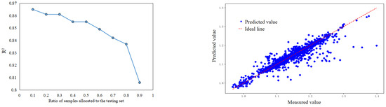
Figure 18.
Proportion and prediction results of the SVR model test set.
Table 6.
The application effect of the multi-well test set of the SVR model.
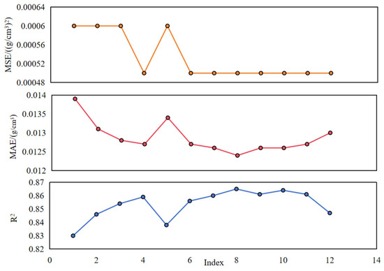
Figure 19.
Evaluation indicators of SVR model.
In summary, the SVR model performs best when the test set ratio is 0.1. At serial number 8, the evaluation metric R2 is the highest, and the fitting effect is good; MAE and MSE are the smallest, indicating the best model performance. Therefore, the relevant parameters for the SVR model are determined as follows: the test set ratio is 0.1, C is 10, γ is 5, and ε is 0.1. At this point, R2 is 0.865, MAE is 0.0124 g/cm3, and MSE is 0.0005 (g/cm3)2.
- (b)
- Establishment of LSTM Model
The LSTM model has 11 input neurons and 1 output neuron. The test set ratio is divided, as shown in Figure 20. The model performs best when the test set ratio is 0.1. The hyperparameters of the LSTM model were optimized, with the best parameter combination and evaluation metrics for the model on the test set shown in Table 7 and Figure 21.
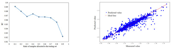
Figure 20.
Proportion and prediction results of the LSTM model test set.
Table 7.
The application effect of the multi-well test set of the LSTM model.
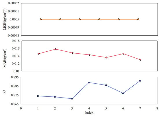
Figure 21.
Evaluation indicators of the LSTM model.
Accordingly, the parameter combination with serial number 7 performs better, with three layers and the number of neurons being 64, 32, and 1, respectively, 300 epochs, and a batch size of 32. In this case, R2 is 0.891, MAE is 0.0130 g/cm3, and MSE is 0.0005 (g/cm3)2.
Based on multi-well data, after training, testing, and parameter optimization of the three models, the model parameters and evaluation metrics were determined as follows: For the SVR model, the test set ratio is 0.1, C is 10, is 5, and is 0.1, with R2 of 0.865, MAE of 0.0124 g/cm3, and MSE of 0.0005 (g/cm3)2; for the LSTM model, the test set ratio is 0.1, with three layers, the number of neurons being 64, 32, and 1, respectively, 300 epochs, batch size of 32, with R2 of 0.891, MAE of 0.0130 g/cm3, and MSE of 0.0005 (g/cm3)2.
4.3.4. Vertical Distribution Pattern of Formation Pressure
Formation pressure of the Carboniferous to Ediacaran carbonate rock formations in the Tarim Basin is predicted using three methods: the Bowers effective stress method, SVR, and an LSTM neural network. The predicted formation pressures from each method were compared against the vertical well-depth profile. As shown in Figure 22, Well T1 displays normal pressure in the Carboniferous interval, a gradual pressure increase from the Ordovician to the Ediacaran, and distinct overpressure characteristics within the Ediacaran formation.
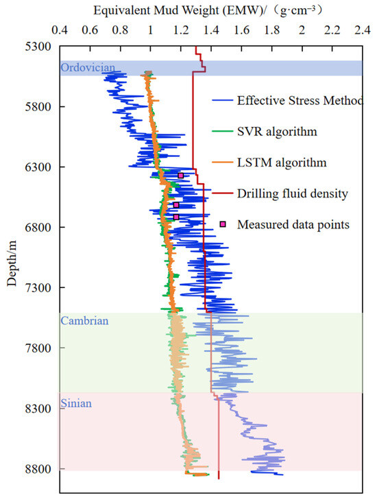
Figure 22.
Formation pressure prediction results from well T1.
Based on the SVR model and LSTM model, formation pressure predictions for both single wells and multiple (six) wells in the Tarim Basin carbonate rock formations were carried out. A comparative analysis of the evaluation metrics for single-well formation pressure prediction using machine learning algorithms shows that the LSTM model has the best fitting effect in terms of R2; the SVR model has the smallest MAE, indicating that the average absolute deviation between predicted values and actual values is smaller. In addition, the estimated MAPE was calculated from MAE using a typical formation density, allowing a direct comparison of percentage errors. The results show that, for single-well predictions, LSTM generally achieves slightly lower MAPE values than SVR, reflecting its higher fitting capability to capture the well-specific trends. Based on Figure 22, the original formation pressures include three measured points. A paired t-test using the prediction errors at these points indicates a statistically significant improvement of LSTM over SVR (p ≈ 0.037), confirming that the higher R2 of LSTM is meaningful even for this small sample. Using the relevant data from Well T1, the SVR and LSTM models were trained and tested for multi-well prediction. The comparison of evaluation metrics is shown in Table 8 and Figure 23.
Table 8.
Model evaluation indexes.
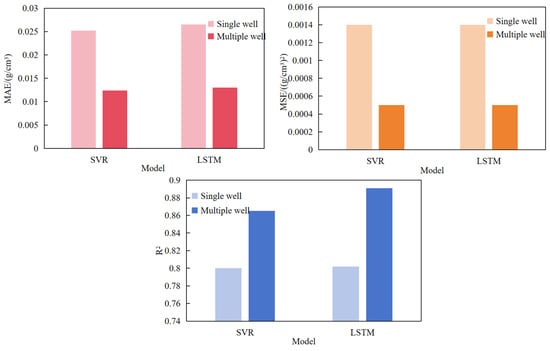
Figure 23.
Comparison of evaluation indexes.
After increasing the data volume, both MSE and MAE have decreased, and the fitting accuracy has been significantly improved. This finding indicates that the model’s fitting effect has been enhanced after increasing the data volume. In terms of R2, the LSTM model has higher fitting accuracy. For MSE, both models show similar performance; however, in terms of MAE, the SVR model performs better (Table 9). Compared to the evaluation metrics of the SVR model, the LSTM model has an R2 of 0.891, MSE of 0.0005 (g/cm3)2, and MAE of 0.0130 g/cm3. This algorithm is better at fitting the changing trend of the data in carbonate rock formation pressure prediction, has greater advantages, and can provide a reference for subsequent engineering applications. Although the LSTM model accurately predicts formation pressure from logging and drilling data, the method remains a data-driven black box lacking explicit physical interpretability. Unlike the Bowers method, results should be interpreted alongside geological and petrophysical understanding to ensure reliability.
Table 9.
Comparison of prediction error between the traditional methods and machine learning method.
Compared to the evaluation metrics of the SVR model, the LSTM model performs the best with a better fitting effect. Therefore, based on the measured formation pressure values, the accuracy differences between traditional methods and the LSTM model in predicting the formation pressure of carbonate rock formations are compared, with the specific data shown in Table 9.
Accordingly, traditional methods such as the Effective Stress and Bowers methods yield MRE ranging from 0.908% to 17.95% when compared with the measured formation pressures of the carbonate intervals, whereas the LSTM model achieves the highest prediction accuracy, with an MRE range of 0.256–3.846%. Compared to traditional methods, the LSTM model has a greater advantage and higher accuracy in formation pressure prediction for carbonate rock formations, and can serve as a reference for subsequent formation pressure predictions in other research areas.
5. Conclusions
Focusing on the Tarim Basin, this research integrates geological, logging, and tectonic data to elucidate the mechanisms responsible for abnormal pressure in carbonate formations. Accordingly, formation pressure prediction for the target block is carried out based on this research, using traditional formation pressure prediction models and machine learning algorithms.
- (1)
- The acoustic velocity-density method and the acoustic velocity-vertical effective stress method, combined with multi-source data integration, were employed to establish a comprehensive evaluation framework. This analysis demonstrates that abnormal overpressure in the target carbonate formations is mainly governed by hydrocarbon generation and tectonic compression.
- (2)
- High-correlation analysis (R2 > 0.5) identified ten key parameters, such as well depth, gamma ray, and rock density, among which those with R2 > 0.8 were determined to be the key parameters for predicting carbonate formation pressure.
- (3)
- With increasing data volume, both MSE and MAE decreased, indicating improved model performance. While the SVR model showed stable results, the LSTM model demonstrated superior predictive capability (R2 = 0.891), providing a more reliable foundation for subsequent engineering applications.
- (4)
- In terms of the evaluation index comparison results, the LSTM model performs better, with a coefficient of determination of 0.891, an average absolute error of 0.0130 g/cm3, and a mean square error of 0.0005 (g/cm3)2. Compared to the measured values, the Bowers method has an average relative error ranging from 0.908% to 14.909%, whereas the average relative error of the LSTM model is less than 3.846%, indicating that the LSTM model can more accurately predict the formation pressure distribution of carbonate rock formations.
Author Contributions
Study conception and design, Z.H. and W.H.; data collection, Q.G. and X.C.; analysis and interpretation of results, Z.M., W.C. and Y.Z.; draft manuscript preparation, J.W. and J.M. All authors have read and agreed to the published version of the manuscript.
Funding
This study was funded by the project of the National Key Laboratory of Oil and Gas Reservoir Accumulation and Effective Development (No. 36650000-24-ZC0699-0014).
Data Availability Statement
Data will be made available upon request.
Acknowledgments
We would like to thank all the authors for their guidance and help on this article.
Conflicts of Interest
Author Qingbin Guo was employed by the company R&D Center for Ultra Deep Complex Reservoir Exploration and Development, CNPC, Key Laboratory of Carbonate, CNPC. The remaining authors declare that the research was conducted in the absence of any commercial or financial relationships that could be construed as a potential conflict of interest. The company had no role in the design of the study; in the collection, analyses, or interpretation of data; in the writing of the manuscript, or in the decision to publish the results.
References
- Eaton, B.A. The effect of overburden stress on geopressure prediction from well logs. J. Pet. Technol. 1972, 24, 929–934. [Google Scholar] [CrossRef]
- Civan, F. Effective-stress coefficients of porous rocks involving shocks and loading/unloading hysteresis. SPE J. 2021, 26, 44–67. [Google Scholar] [CrossRef]
- Bowers, G.L. Pore pressure estimation from velocity data: Accounting for overpressure mechanisms besides undercompaction. SPE Drill. Complet. 1995, 10, 89–95. [Google Scholar] [CrossRef]
- Fillippone, W.R. Estimation of formation parameters and the prediction of over-pressure from seismic data. In SEG Technical Program Expanded Abstracts, Proceedings of the 52nd SEG Annual International Meeting, Dallas, TX, USA, 17–21 October 1982; Society of Exploration Geophysicists: Houston, TX, USA, 1982; pp. 502–503. [Google Scholar]
- Hottman, C.E.; Johnson, R.K. Estimation of formation pressures from log-derived shale properties. J. Pet. Technol. 1965, 17, 717–722. [Google Scholar] [CrossRef]
- Bohnsack, D.; Potten, M.; Freitag, S.; Einsiedl, F.; Zosseder, K. Stress sensitivity of porosity and permeability under varying hydrostatic stress conditions for different carbonate rock types of the geothermal Malm reservoir in Southern Germany. Geotherm. Energy 2021, 9, 15. [Google Scholar] [CrossRef]
- Abdelaal, A.; Elkatatny, S.; Abdulraheem, A. Real-time prediction of formation pressure gradient while drilling. Sci. Rep. 2022, 12, 11318. [Google Scholar] [CrossRef]
- Hongquan, X.; Xiaobo, Y.; Zhong, L.; Song, Y. Calculation of pore pressure logging in carbonate rock formations based on effective stress method. Drill. Prod. Technol. 2005, 28, 28–30+116. [Google Scholar]
- Zhao, R.; Deng, S.; Yun, L.; Lin, H.; Zhao, T.; Yu, C.; Kong, Q.; Wang, Q.; Li, H. Description of the reservoir along strike-slip fault zones in China T-Sh oilfield, Tarim Basin. Carbonates Evaporites 2021, 36, 2. [Google Scholar] [CrossRef]
- Zhang, Z.; Yan, C.; Cheng, Y.; Han, Z.; Wu, S. Formation pressure prediction method based on machine learning. J. Phys. Conf. Ser. 2024, 2834, 012083–012093. [Google Scholar] [CrossRef]
- Liu, T.; Ye, X.; Cheng, L.; Hu, Y.; Guo, D.; Huang, B.; Li, Y.; Su, J. Intelligent pressure monitoring method of BP neural network optimized by genetic algorithm: A case study of X well area in Yinggehai Basin. Processes 2024, 12, 2439. [Google Scholar] [CrossRef]
- Pan, H.; Deng, S.; Li, C.; Sun, Y.; Zhao, Y.; Shi, L.; Hu, C. Research progress of machine-learning algorithm for formation pore pressure prediction. Pet. Sci. Technol. 2025, 43, 341–359. [Google Scholar] [CrossRef]
- Jiang, D.; Chen, H.; Xing, J.; Wang, Y.; Wang, Z.; Tuo, H. A new method for dynamic predicting porosity and permeability of low permeability and tight reservoir under effective overburden pressure based on BP neural network. Geoenergy Sci. Eng. 2023, 226, 211721. [Google Scholar] [CrossRef]
- Keshavarzi, R.; Jahanbakhshi, R. Real-time prediction of pore pressure gradient through an artificial intelligence approach: A case study from one of middle east oil fields. Eur. J. Environ. Civ. Eng. 2013, 17, 675–686. [Google Scholar] [CrossRef]
- Bungasalu, A.B.; Rosid, S.M.; Basuki, S.D. Drilling optimization of tight sands and shale gas reservoir in Jambi Sub-Basin based on pore pressure estimation using drilling efficiency mechanical specific energy (DEMSE) and Bowers methods. E3S Web Conf. 2019, 125, 15001–15015. [Google Scholar] [CrossRef]
- Farsi, M.; Mohamadian, N.; Ghorbani, H.; Wood, D.A.; Davoodi, S.; Moghadasi, J.; Alvar, M.A. Predicting formation pore-pressure from well-log data with hybrid machine-learning optimization algorithms. Nat. Resour. Res. 2021, 30, 1–27. [Google Scholar] [CrossRef]
- Samir, K.; Ashraf, A.S.; Abdulrahman, M.; Sayed, G.; Attia, M.A. New models for predicting pore pressure and fracture pressure while drilling in mixed lithologies using artificial neural networks. ACS Omega 2022, 7, 31691–31699. [Google Scholar] [CrossRef] [PubMed]
- Zhang, X.; Li, B.; Peng, J.; Qu, F.; Zhang, K.; Yang, S.; Xu, Q. Experimental analysis of dissolution reconstruction of deep dolomite reservoirs: A case study of the Cambrian dolomite reservoirs in the Tarim Basin. Front. Earth Sci. 2022, 10, 1015460. [Google Scholar] [CrossRef]
- Özkiliç, Y.O.; Zeybek, Ö.; Karalar, M.; Çelik, A.İ.; Althaqafi, E. Experimental and ARX model-based prediction of concrete strength with waste marble powder as replacement of aggregates. Struct. Eng. Mech. 2025, 95, 015. [Google Scholar]
- Özkılıç, Y.O.; Bahrami, A.; Güzel, Y.; Soğancı, A.S.; Karalar, M.; Althaqafi, E.; Çelik, A.İ.; Zeybek, Ö.; Jagadesh, P. Waste ceramic powder for sustainable concrete production as supplementary cementitious material. Front. Mater. 2025, 11, 1450824. [Google Scholar] [CrossRef]
- Özkılıç, Y.O.; Zeybek, Ö.; Karalar, M.; Çelik, A.I.; Althaqafi, E. Improvement and predictive modeling of the mechanical performance of waste fire clay blended concrete. Rev. Adv. Mater. Sci. 2025, 64, 20250114. [Google Scholar] [CrossRef]
- Chen, H.; Wang, K.; Zhao, M.; Chen, Y.; He, Y. A CNN-LSTM-attention based seepage pressure prediction method for Earth and rock dams. Sci. Rep. 2025, 15, 12960. [Google Scholar] [CrossRef]
- Sadeghtabaghi, Z.; Kadkhodaie, A.; Mehdipour, V.; Kadkhodaie, R. An innovative approach for investigation of overpressure due to hydrocarbon generation: A regional study on Kazhdumi formation, southwestern Zagros Basin, Iran. J. Pet. Explor. Prod. Technol. 2024, 14, 1331–1347. [Google Scholar] [CrossRef]
- Su, A.; Chen, H.; Yang, W.; Feng, Y.; Zhao, J.; Lei, M. Hydrocarbon gas leakage from high-pressure system in the Yanan Sag, Qiongdongnan Basin, South China Sea. Geol. J. 2021, 56, 5094–5108. [Google Scholar] [CrossRef]
- Leusheva, E.; Alikhanov, N.; Morenov, V. Barite-free muds for drilling-in the formations with abnormally high pressure. Fluids 2022, 7, 268. [Google Scholar] [CrossRef]
- Lu, X.; Zhao, M.; Zhang, F.; Gui, L.; Liu, G.; Zhuo, Q.; Chen, Z. Characteristics, origin and controlling effects on hydrocarbon accumulation of overpressure in foreland thrust belt of southern margin of Junggar Basin, NW China. Pet. Explor. Dev. 2022, 49, 991–1003. [Google Scholar] [CrossRef]
- Zou, L.; Guo, J.; Zhang, L.; Huang, G.; Jiao, S.; Tian, Z.; Wang, D.; Liu, P. Paleoproterozoic ultrahigh-temperature mafic granulites with a high-pressure prograde path from the Alxa Block: Implications on the tectonic evolution of the Khondalite Belt, North China Craton. J. Metamorph. Geol. 2024, 42, 551–581. [Google Scholar] [CrossRef]
- Chen, Y.; Yu, F.; Luo, B.; Zou, X. Formation pressure prediction and high pressure formation mechanisms of shale reservoirs in Fuling area, Sichuan Basin. Pet. Geol. Exp. 2018, 40, 110–117. [Google Scholar]
- Hua, Y.; Guo, X.; Tao, Z.; He, S.; Dong, T.; Han, Y.; Yang, R. Mechanisms for overpressure generation in the bonan sag of Zhanhua depression, Bohai Bay Basin, China. Mar. Pet. Geol. 2021, 128, 105032. [Google Scholar] [CrossRef]
- Yu, Y.; Si, X.; Hu, C.; Zhang, J. A review of recurrent neural networks: LSTM cells and network architectures. Neural Comput. 2019, 31, 1235–1270. [Google Scholar] [CrossRef] [PubMed]
- Li, H.; Tan, Q.; Deng, J.; Dong, B.; Li, B.; Guo, J.; Zhang, S.; Bai, W. A comprehensive prediction method for pore pressure in abnormally high-pressure blocks based on machine learning. Processes 2023, 11, 2603. [Google Scholar] [CrossRef]
- Siddique, A.B.; Alam Munshi, T.; Rakin, N.I.; Hashan, M.; Chnapa, S.S.; Jahan, L.N. Application of supervised machine learning and unsupervised data compression models for pore pressure prediction employing drilling, petrophysical, and well log data. Sci. Rep. 2025, 15, 24706. [Google Scholar] [CrossRef] [PubMed]
- Zaidi, S. Development of support vector regression (SVR)-based model for prediction of circulation rate in a vertical tube thermosiphon reboiler. Chem. Eng. Sci. 2012, 69, 514–521. [Google Scholar] [CrossRef]


Disclaimer/Publisher’s Note: The statements, opinions and data contained in all publications are solely those of the individual author(s) and contributor(s) and not of MDPI and/or the editor(s). MDPI and/or the editor(s) disclaim responsibility for any injury to people or property resulting from any ideas, methods, instructions or products referred to in the content. |
© 2025 by the authors. Licensee MDPI, Basel, Switzerland. This article is an open access article distributed under the terms and conditions of the Creative Commons Attribution (CC BY) license (https://creativecommons.org/licenses/by/4.0/).