A Model-Search Multi-Objective Derivative-Free Optimization Algorithm with Sparse Modeling

Abstract

Multi-objective derivative-free optimization has broad applications in engineering fields, with its main challenge being how to solve problems efficiently without gradient information. This article proposes a novel multi-objective derivative-free optimization algorithm that integrates sparse modeling techniques with a new non-dominated comparison function within a direct multisearch framework. To fully leverage information from historically evaluated points, the algorithm employs quadratic surrogate models constructed from these points to enhance the search step, with model coefficients determined through either linear programming or least-squares methods. Simultaneously, a Pareto dominance-based comparison function is introduced to improve the selection capability of candidate solutions. Experimental results on ZDT and WFG benchmark problems demonstrate that, through comparisons of hypervolume values and performance profiles, the proposed algorithm exhibits competitiveness and robustness under limited function evaluation budgets compared to existing state-of-the-art methods.

1. Introduction

As computational simulations and data-driven modeling have become critical research tools, practical optimization increasingly involves derivative-free objectives from these sources while balancing competing goals. This defines multi-objective derivative-free optimization (DFO) problems, which are prevalent in engineering domains like chemical engineering and steel metallurgy. A general multi-objective DFO problem can be formulated as follows:

$$\begin{array}{c}\hfill \begin{array}{cc}\hfill & \min \mathit{F}\left(\mathit{x}\right)=(f_1\left(\mathit{x}\right),\cdots ,f_m\left(\mathit{x}\right))\hfill \\ \hfill & s.t.\mathit{x}\in \Omega \hfill \end{array}\end{array}$$

(1)

where $\mathit{x}\in {\mathbb{R}}^n$ is an n-dimensional decision vector within the feasible decision set $\Omega \subseteq {\mathbb{R}}^n$. The corresponding feasible objective set is then defined as the mapping of $\Omega$ under the objective function $\mathit{F}\left(\mathit{x}\right)=(f_1\left(\mathit{x}\right),\cdots ,f_m\left(\mathit{x}\right))$. Moreover, the objective function $f_i\left(x\right):{\mathbb{R}}^n\to \mathbb{R}\cup \{\infty \}$ for $i=1,\cdots ,m(m\ge 2)$ satisfies the following: (i) At least one $f_i\left(\mathit{x}\right)$ is a black-box (derivative-free) function. (ii) For any $j\in \{1,2,\dots ,m\}$, there exists $i\ne j$ such that $f_i$ and $f_j$ conflict, meaning that no point in $\Omega$ can simultaneously minimize all objectives. This article focuses specifically on the bound-constrained case, i.e.,

$$\Omega =\left\{\mathit{x}\right|{\mathit{l}}_b\le \mathit{x}\le {\mathit{u}}_b\}$$

(2)

where ${\mathit{l}}_b\in {\mathbb{R}}^n$ and ${\mathit{u}}_b\in {\mathbb{R}}^n$ denote element-wise lower- and upper-bound vectors for the decision variable $\mathit{x}$.

The optimization methods for solving such problems can be broadly classified into three categories: direct search methods, model-based methods, and population-based heuristic methods. Direct search methods generate candidate solutions through systematic geometric sampling patterns, as exemplified in [1,2,3,4]. Model-based methods, also referred to as surrogate-based methods, construct approximation models from evaluated points and generate new candidates by optimizing these surrogates, often embedded within trust-region frameworks [5,6,7,8]. Population-based heuristic algorithms, which simulate evolutionary processes or collective behaviors within solution sets to generate candidate solutions, have long been commonly used for solving multi-objective DFO problems [9,10,11].

However, such heuristic algorithms typically require a large number of function evaluations and lack mathematical convergence guarantees, making them unsuitable for expensive black-box functions. To mitigate this limitation, surrogate-assisted population-based algorithms have been developed. For instance, ref. [12] proposed a surrogate-assisted multi-objective evolutionary algorithm with a two-level model management strategy to balance convergence and diversity under a limited evaluation budget. Similarly, ref. [13] introduced a linear subspace surrogate modeling approach for large-scale expensive optimization, which constructs effective models in high-dimensional spaces using minimal historical data. Additionally, decision variable clustering has been applied to enhance multi-objective optimization (MOO) algorithms in addressing large-scale problems [14].

Meanwhile, multi-objective DFO methods derived from model-based trust-region frameworks are also attracting growing research attention. For example, building on the scalarization approach in [15], a DFO method was developed under the trust-region framework for bi-objective optimization problems [16]. Subsequently, ref. [17] proposed a direct multi-objective trust-region algorithm for problems where at least one objective is an expensive black-box function. More recently, ref. [7] presented a modified trust-region approach for approximating the complete Pareto front in multi-objective DFO problems.

Furthermore, directional direct search methods, whose global convergence and computational complexity have been thoroughly characterized [18,19], have also been extended to multi-objective DFO. For instance, mesh adaptive search was extended to bi-objective optimization problems, though the uniformity of solution distribution was limited by the design of aggregation functions in pre-decision techniques [15]. Later, ref. [20] developed the multi-objective MADS algorithm using the normal boundary intersection (NBI) method and established necessary convergence conditions. However, the construction of convex hulls for individual objective minimization in NBI led to significant sensitivity of MADS performance to convex hull parameters. To address this, ref. [1] proposed the direct multisearch (DMS) framework, integrating pattern search with mesh adaptive strategies. The original DMS framework did not incorporate a search step. To overcome this limitation, ref. [21] developed the BoostDMS algorithm, which enhances performance through the integration of a model-based search step. Building upon this, ref. [22] further extended the framework to a parallel multi-objective DFO algorithm that unifies both search and poll steps. To tackle challenges from local optima in multi-modal problems, ref. [2] introduced multi-start strategies into algorithm design. Inspired by [2,23], ref. [3] proposed a novel mesh adaptive search-based optimizer to improve convergence properties. For better handling of nonlinear constraints in multi-objective DFO, ref. [24] replaced the extreme barrier constraints in DMS with a filter strategy incorporating inexact feasibility restoration. Additionally, to improve computational efficiency in practical applications, ref. [4] established an adaptive search direction selection mechanism, validated through numerical experiments on benchmark functions and automotive suspension design.

This article presents a multi-objective DFO algorithm designed to approximate the complete Pareto front within a limited function evaluation budget. The proposed algorithm, developed within the DMS framework and denoted as DMSCFSM, incorporates sparse modeling and a novel non-dominated comparison function technique. It integrates several strategies from previous works, including the use of previously evaluated points for surrogate model construction [21], the building of both incomplete and complete models [25], the generation of positively spanning search directions [1], and a Pareto dominance-based comparison mechanism [26].

Inspired by [25], a sparse modeling approach is adopted in the search step to formulate surrogate models. This method plays a crucial role in mitigating the curse of dimensionality and differs from the modeling strategy employed in [21]. Moreover, it has been observed that conventional non-dominated set updates, which rely solely on Pareto dominance, often overlook differences in dominance strength, which is defined as the number of solutions a point dominates within the mutually non-dominated set. This oversight can result in retaining solutions with weak dominance strength, making them vulnerable to replacement by new non-dominated points in subsequent iterations. To address this issue, a new comparison function is introduced in the proposed algorithm. A detailed description of DMSCFSM is provided in Section 3.

The structure of this article is organized as follows: Section 2 presents the preliminaries. The modified algorithm is elaborated in Section 3. Section 4 delves into numerical results and the experimental implementation of the method, which includes a comparison of the algorithm’s numerical performance with state-of-the-art algorithms. Finally, conclusions are provided in Section 5.

2. Preliminaries

In this section, relevant preliminaries are given, such as preliminaries on MOO and the DMS framework.

2.1. Preliminaries on MOO

In MOO, no solution exists that simultaneously minimizes all m objectives due to inherent conflicts between at least two objective functions. Consequently, unlike single-objective optimization, which seeks a single optimal solution, MOO aims to obtain a set of Pareto-optimal solutions that capture the trade-offs between competing objectives. For a minimization MOO, a solution ${\mathit{x}}_1$ dominates a solution ${\mathit{x}}_2$ if and only if

$$\forall i:f_i\left({\mathit{x}}_1\right)\le f_i\left({\mathit{x}}_2\right),\exists j:f_j\left({\mathit{x}}_1\right)<f_j\left({\mathit{x}}_2\right)$$

(3)

where $i,j=1,2,\dots ,m$. The solutions that are not dominated by any other solutions are known as Pareto-optimal solutions. The points in the Pareto-optimal set correspond to the Pareto front of the MOO problem in the objective space. Figure 1 illustrates the relationship between Pareto-optimal solutions and the Pareto front.

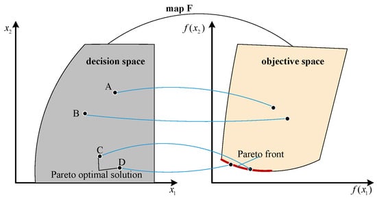
Figure 1. Graphical depiction of multi-objective optimization.

2.2. Extreme Barrier Approach

Constraints are handled using the extreme barrier approach [1]. The original objective function is extended to a barrier function ${\mathit{F}}_{\Omega }:{\mathbb{R}}^n\to {(\mathbb{R}\cup \{+\infty \})}^m$, defined as

$${\mathit{F}}_{\Omega }\left(\mathbf{x}\right)=\left\{\begin{array}{cc}\mathit{F}\left(\mathit{x}\right),\hfill & \mathit{x}\in \Omega ,\hfill \\ {(+\infty ,\dots ,+\infty )}^{\top },\hfill & \mathit{x}\notin \Omega .\hfill \end{array}\right.$$

(4)

This definition ensures that infeasible points are automatically dominated in any optimization comparison, thereby guiding the search toward the feasible region $\Omega$.

2.3. DMS Framework Overview

Since its introduction in [1], the DMS method has demonstrated superior performance in benchmarking new solvers and industrial implementations [21]. Figure 2 illustrates the key algorithmic steps of the DMS method, with a complete description provided in [1].

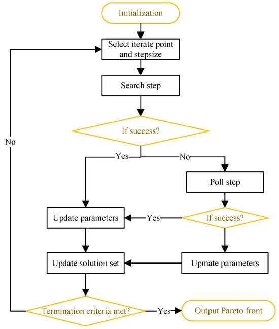
Figure 2. Major algorithmic steps of DMS.

At each iteration, the algorithm begins by selecting an iterate point and a corresponding step-size parameter from the current list of feasible non-dominated points. Different ordering strategies for this list produce various algorithmic variants. In the numerical experiments, a spread metric is used to order points in a way that minimizes gaps between consecutive solutions along the current approximation of the Pareto front.

Following the selection of an iterate point, the algorithm executes a search step. If this step fails to improve the non-dominated set, a poll step is initiated around the current iterate. Notably, the search step is executed only after a poll step has been completed and when the current step size exceeds a predefined stopping threshold.

During the poll step, DMS employs a positive spanning set [27] as direction vectors to generate new points from the poll center. It evaluates the objective function at displacements scaled by a step-size parameter along these vectors, implementing a complete polling strategy.

At the end of each iteration, all relevant parameters are updated. Specifically, the step-size parameter is increased (or maintained) upon a successful iteration and decreased otherwise. Other parameters are then adjusted accordingly.

3. Proposed Algorithm Description

In this section, the proposed model-search DFO algorithm is presented, along with a detailed description of the surrogate modeling method for the search step, a definition of the Pareto dominance-based comparison function, and a comprehensive outline of the complete algorithmic framework.

3.1. Surrogate Modeling Method for Search Step

In this article, the model construction approach is consistent with that employed in trust-region model-based algorithms. Without loss of generality, one objective function $f_i\left(\mathit{x}\right),(i=1,2,\cdots ,m)$ (denoted as $\tilde{f}\left(\mathit{x}\right)$) is considered to illustrate the surrogate modeling approach. In trust-region model-based algorithms, obtaining each iteration step requires finding a solution to the following subproblem:

$$\begin{array}{c}\underset{\mathit{s}\in {\mathbb{R}}^n}{\min }{m}_k\left(\mathit{s}\right)={\tilde{f}}_k+{\mathit{g}}_k^T\mathit{s}+{\displaystyle \frac{1}{2}}{\mathit{s}}^{\top }{\mathit{B}}_k\mathit{s}\hfill \\ \mathrm{s}.\mathrm{t}.\parallel \mathit{s}\parallel \le {\Delta }_k\hfill \end{array}$$

(5)

where $\mathit{s}=\mathit{x}-{\mathit{x}}_k$, and ${\Delta }_k$ denotes the trust-region radius at the k-th iteration. Here, ${\mathit{g}}_k$ and ${\mathit{B}}_k$ are the gradient and the approximate Hessian of $\tilde{f}\left(\mathit{x}\right)$, respectively, which are obtained from the surrogate model $m_k\left(\mathit{x}\right)$.

The quadratic polynomial surrogate models are formulated using selected historical points from the evaluation cache to compute ${\mathit{g}}_k$ and ${\mathit{B}}_k$. The model may be either an incomplete or a complete quadratic approximation, depending on the number of available evaluated points. Let $\mathit{Y}=\{{\mathit{Y}}^1,{\mathit{Y}}^2,\cdots ,{\mathit{Y}}^p\}$ represent the sample set filtered from the cache, where the objective functions $f_1\left(\mathit{x}\right),\cdots ,f_m\left(\mathit{x}\right)$ have been evaluated. Each point ${\mathit{Y}}^i$ in this set is defined as ${\mathit{Y}}^i=(y_{i1},y_{i2},\cdots ,y_{in})$. Define $\varphi =\{{\varphi }_1,{\varphi }_2,\cdots ,{\varphi }_q\}$ as a basis for the polynomial space ${\mathcal{P}}_n^2$ (degree $\le 2$ polynomials in ${\mathbb{R}}^n$), where $q={\displaystyle \frac{(n+1)(n+2)}{2}}$ is the space dimension. The $m_k\left(\mathit{x}\right)$ model can be formulated as

$$m_k\left(\mathit{x}\right)=\sum _{i=1}^q{\zeta }_i{\varphi }_i$$

(6)

The interpolation conditions $m_k\left({\mathit{Y}}^i\right)=\tilde{f}\left({\mathit{Y}}^i\right)(i=1,2,\cdots ,p)$ lead to the following linear system (7):

$$M(\varphi ,\mathit{Y})\mathit{\zeta }=\tilde{\mathit{f}}\left(\mathit{Y}\right)$$

(7)

where $\mathit{\zeta }={({\zeta }_1,{\zeta }_2,\cdots ,{\zeta }_q)}^{\top }\in {\mathbb{R}}^q$ is the coefficient vector, $\tilde{\mathit{f}}={(\tilde{f}\left({\mathit{Y}}^1\right),\tilde{f}\left({\mathit{Y}}^2\right),\cdots ,\tilde{f}\left({\mathit{Y}}^p\right))}^{\top }$ contains observed values, and $M(\varphi ,\mathit{Y})$ is the $p\times q$ interpolation matrix with elements $M_{ij}={\varphi }_j\left({\mathit{Y}}^i\right)$.

For exact interpolation (if $p=q$), the matrix $M(\varphi ,\mathit{Y})$ must be invertible. However, when $p\ne q$, the system becomes either underdetermined (if $p<q$) or overdetermined (if $p>q$), and a direct solution is not feasible.

When $p>q$, the parameter coefficients $\mathit{\zeta }\in {\mathbb{R}}^q$ can be determined by solving the following least-squares problem (8):

$$\underset{\mathit{\zeta }}{\min }{\parallel M(\varphi ,\mathit{Y})\mathit{\zeta }-\tilde{\mathit{f}}\left(\mathit{Y}\right)\parallel }_2^2$$

(8)

By taking the partial derivatives with respect to $\mathit{\zeta }$ and setting them to zero, the following system of Equation (9) is obtained:

$$M^{\top }(\varphi ,\mathit{Y})M(\varphi ,\mathit{Y})\mathit{\zeta }=M^{\top }(\varphi ,\mathit{Y})\tilde{\mathit{f}}\left(\mathit{Y}\right)$$

(9)

If $M(\varphi ,\mathit{Y})$ has full column rank, then $M^{\top }(\varphi ,\mathit{Y})M(\varphi ,\mathit{Y})$ is non-singular.

When $p<q$, a Dantzig selector approach is employed to construct the surrogate model, which possesses the oracle properties [28]. This method differs from the surrogate modeling technique presented in [21], while offering variable selection capabilities for handling sparse optimization problems. The resulting parameter estimation problem leads to the non-smooth convex optimization problem (10).

$$\begin{array}{cc}\underset{\mathit{\zeta }}{\min }\hfill & {\parallel \mathit{\zeta }\parallel }_1\hfill \\ \mathrm{s}.\mathrm{t}.\hfill & \parallel M^{\top }{(\varphi ,\mathit{Y})\mathit{r}\parallel }_{\infty }\le \epsilon \hfill \\ \hfill & \mathit{r}=\tilde{\mathit{f}}\left(\mathit{Y}\right)-M(\varphi ,\mathit{Y})\mathit{\zeta }\hfill \end{array}$$

(10)

where $\epsilon >0$ is a tolerance parameter whose selection affects the accuracy of the predictive model [28] and influences the algorithm’s performance. Adaptive selection is required when solving different problems. In this article, it was uniformly set to eps during the numerical experiments. Problem (10) is an NP-hard optimization problem. Motivated by the well-established theoretical guarantees of linear programming, this issue is addressed by reformulating the problem (10) in the form of (11) by introducing non-negative variables ${\mathit{\zeta }}^{+}\in {\mathbb{R}}^q$ and ${\mathit{\zeta }}^{-}\in {\mathbb{R}}^q$. Alternatively, problem (10) can also be solved directly by other methods, such as the alternating direction method of multipliers (ADMM) [29] and basis-pursuit denoising [30].

$$\begin{array}{cc}\underset{\tilde{\mathit{\zeta }}}{\min }\hfill & {\mathbf{1}}^{\top }\tilde{\mathit{\zeta }}\hfill \\ \mathrm{s}.\mathrm{t}.\hfill & \mathcal{M}\tilde{\mathit{\zeta }}\le \mathit{\beta }\hfill \\ \hfill & \tilde{\mathit{\zeta }}⪰\mathbf{0}\hfill \end{array}$$

(11)

where $\mathit{\zeta }={\mathit{\zeta }}^{+}-{\mathit{\zeta }}^{-}$ with ${\zeta }_i^{+}=max\{{\zeta }_i,0\}$ and ${\zeta }_i^{-}=max\{-{\zeta }_i,0\}$. And $\tilde{\mathit{\zeta }}={({\mathit{\zeta }}^{{+}^{\top }},{\mathit{\zeta }}^{{-}^{\top }})}^{\top }\in {\mathbb{R}}^{2q}$, $\mathbf{1}\in {\mathbb{R}}^{2q}$ denotes the all-ones vector of dimension $2q$. Moreover, $\mathit{\beta }=\left(\begin{array}{c}{M}^{\top }(\varphi ,\mathit{Y})\tilde{\mathit{f}}\left(\mathit{Y}\right)+\epsilon {\mathbf{1}}_q\\ -M^{\top }(\varphi ,\mathit{Y})\tilde{\mathit{f}}\left(\mathit{Y}\right)+\epsilon {\mathbf{1}}_q\end{array}\right)$ and $\mathcal{M}=\left(\begin{array}{cc}{M}^{\top }(\varphi ,\mathit{Y})M(\varphi ,\mathit{Y})& -M^{\top }(\varphi ,\mathit{Y})M(\varphi ,\mathit{Y})\\ -M^{\top }(\varphi ,\mathit{Y})M(\varphi ,\mathit{Y})& M^{\top }(\varphi ,\mathit{Y})M(\varphi ,\mathit{Y})\end{array}\right)$.

Algorithm 1 outlines the pseudocode for constructing quadratic surrogate models, from which ${\mathit{g}}_k$ (gradient) and ${\mathit{B}}_k$ (approximate Hessian) are derived. The trial points are then obtained by solving the trust-region subproblem (5), which minimizes the surrogate model within the current-iteration trust region.

Algorithm 1 Surrogate model construction

Require:  Evaluated points $\mathit{Y}=\{{\mathit{Y}}^1,\dots ,{\mathit{Y}}^p\}$ with function values $\tilde{\mathit{f}}\left(\mathit{Y}\right)$; Dimension n Ensure:  Gradient ${\mathit{g}}_k$ and Hessian ${\mathit{B}}_k$   1: $n\leftarrow$ dimension of decision space   2: $q\leftarrow {\displaystyle \frac{(n+1)(n+2)}{2}}$   3: $p\leftarrow \mathrm{card}\left(\mathit{Y}\right)$ ($\mathrm{card}\left(\mathit{Y}\right)$ represents the number of samples in the sample set Y)   4: if $p==q$ then   5:     Form interpolation matrix $M(\varphi ,\mathit{Y})$ with basis $\varphi =\{{\varphi }_1,\dots ,{\varphi }_q\}$   6:     Solve $\mathit{\zeta }$ from Equation (7) via SVD   7: else if $p>q$ then   8:     Solve $\mathit{\zeta }$ from Equation (9) via SVD   9: else if $p<q$ then 10:    Solve $\mathit{\zeta }$ from from linear program (11) via $\mathtt{linprog}$ to get $\mathit{\zeta }={\mathit{\zeta }}^{+}-{\mathit{\zeta }}^{-}$ (where $\tilde{\mathit{\zeta }}={({\mathit{\zeta }}^{+\top },{\mathit{\zeta }}^{-\top })}^{\top }$) 11: Derive ${\mathit{g}}_k$ from $\mathit{\zeta }$ (coefficients of linear terms in $\varphi$) 12: Derive ${\mathit{B}}_k$ from $\mathit{\zeta }$ (coefficients of quadratic terms in $\varphi$) 13: return ${\mathit{g}}_k$ and ${\mathit{B}}_k$ for constructing subproblem $m_k\left(\mathit{s}\right)$

3.2. Pareto Dominance-Based Comparison Function

Let ${\mathit{x}}_0$ and ${\alpha }_0$ denote the initial point and the corresponding step-size parameter, respectively. Let $L_k$ be the list of non-dominated points along with their corresponding step-size parameters, where $L_0=({\mathit{x}}_0,{\alpha }_0)$. Define $L_{\mathrm{add}}^{\left(k\right)}$ as the set of new candidate points and their step-size parameters generated during the k-th iteration. Now suppose ${\mathit{x}}_1$ and ${\mathit{x}}_2$ are two points in $L_{\mathrm{add}}^{\left(k\right)}$ that are mutually non-dominated with respect to the points in $L_k$, but ${\mathit{x}}_1$ dominates more points in $L_k$ than ${\mathit{x}}_2$ does. According to the principle of Pareto dominance, both ${\mathit{x}}_1$ and ${\mathit{x}}_2$ would typically be added to the updated non-dominated list $L_{k+1}$. However, in practice, ${\mathit{x}}_2$ is more likely to be dominated by other points in subsequent iterations. This information is overlooked when selecting non-dominated points solely based on Pareto dominance.

To address this issue, a Pareto dominance-based comparison function $\Phi ({\mathit{x}}_i,{\mathit{x}}_j\mid L_k)$ is proposed, defined as follows:

$$\Phi ({\mathit{x}}_i,{\mathit{x}}_j\mid L_k)=\left\{\begin{array}{cc}1,\hfill & \mathrm{mark}({\mathit{x}}_i,L_k)\ge \mathrm{mark}({\mathit{x}}_j,L_k)\hfill \\ 0,\hfill & \mathrm{mark}({\mathit{x}}_i,L_k)<\mathrm{mark}({\mathit{x}}_j,L_k)\hfill \end{array}\right.$$

(12)

where ${\mathit{x}}_i$ and ${\mathit{x}}_j$ are two feasible candidate points that are non-dominated with respect to points in $L_k$. The function $\mathrm{mark}({\mathit{x}}_i,L)$ is defined as Equation (13).

$$\mathrm{mark}({\mathit{x}}_i,L)=\mathrm{card}\left(\{{\mathit{x}}_i\prec \mathit{y}|\mathit{y}\in L,\mathit{y}\ne {\mathit{x}}_i\}\right)$$

(13)

where $\{{\mathit{x}}_i\prec y|\mathit{y}\in L_k\}$ is the set of solutions in $L_k$ dominated by ${\mathit{x}}_i$, and $\mathrm{card}(·)$ denotes set cardinality.

Based on Equation (12), the comparison function $\Phi ({\mathit{x}}_i,{\mathit{x}}_j\mid L_k)$ determines which candidate point are incorporated into the current non-dominated set $L_k$ to form $L_{k+1}$: when $\Phi ({\mathit{x}}_i,{\mathit{x}}_j\mid L_k)=1$ and $\mathrm{mark}({\mathit{x}}_i,L_k)>\mathrm{mark}({\mathit{x}}_j,L_k)$, the set is updated as $L_{k+1}=\left(L_k\setminus \{{\mathit{x}}_i\prec y|\mathit{y}\in L_k\}\right)\cup \left\{{\mathit{x}}_i\right\}$; if, instead, $\mathrm{mark}({\mathit{x}}_i,L_k)=\mathrm{mark}({\mathit{x}}_j,L_k)$, then $L_{k+1}=\left(L_k\setminus \{{\mathit{x}}_i\prec y|\mathit{y}\in L_k\}\right)\cup \{{\mathit{x}}_i,{\mathit{x}}_j\}$, whereas when $\Phi ({\mathit{x}}_i,{\mathit{x}}_j\mid L_k)=0$, the update becomes $L_{k+1}=\left(L_k\setminus \{{\mathit{x}}_j\prec y|\mathit{y}\in L_k\}\right)\cup \left\{{\mathit{x}}_j\right\}$.

3.3. The General Framework of the DMSCFSM Algorithm

DMSCFSM operates within the DMS framework. The algorithm begins with an initialization phase, and then enters an iterative cycle of search and poll steps. This iteration continues until a stopping or convergence criterion is met. At the k-th iteration, the algorithm aims to refine the approximate Pareto front $L_k$. The complete procedure is formalized in Algorithm 2.

Algorithm 2 DMSCFSM Algorithm Framework

1: Initialization:   2:    Parameters initialization: Set initial step size ${\alpha }_0>0$, contraction coefficients $0<\beta <1$, expansion coefficient $\gamma \ge 1$, and define $\mathcal{D}$ as the set of positive spanning sets. Generate initial sample points $P_{\mathrm{ini}}$ using LHS. Initialize iteration counter $k=0$, cache $L_{\mathrm{cache}}=\varnothing$, candidate set $\mathit{S}=\varnothing$, and success flag $\mathit{success}=0$.   3:    Feasible point evaluation and non-dominated solution identification: Filter feasible points $P_0\subseteq P_{\mathrm{ini}}$ within the domain, evaluate $\left\{f_i\left(\mathit{x}\right)\right|i=1,\dots ,m;\mathit{x}\in P_0\}$ while updating $L_{\mathrm{cache}}$. Set function evaluation counter $n_f=\mathrm{card}\left(P_0\right)$. Compute the non-dominated solution set $\mathrm{NDS}\left(P_0\right)$.   4:    Non-dominated list construction: Initialize the non-dominated solution list as $L_0=\{({\mathit{x}}_i;{\alpha }_0)\mid {\mathit{x}}_i\in \mathrm{NDS}\left(P_0\right)\}$   5: Main Loop:   6: while $n_f<\max \_\mathrm{fevals}$ or $max\left\{\mathit{\alpha }\right\}<ϵ$ do   7:    Sort the points in $L_k$ in descending order according to their projected gaps across all dimensions of the objective space, and select the top-ranked point as the polling center ${\mathit{x}}_{\mathrm{poll}}$.   8:    Search Step:   9:    Set $l\leftarrow 0$, ${\mathit{x}}_{\mathrm{search}}\leftarrow {\mathit{l}}_b$, $\mathit{s}\leftarrow \mathit{x}-{\mathit{x}}_{\mathrm{search}}$ 10:    for $i=1\mathrm{to}m$ do 11:      Construct quadratic model $m_i\left(\mathit{x}\right)$ using the data points in $L_{\mathrm{cache}}\cap B({\mathit{x}}_{\mathrm{search}};{\Delta }_k)$ 12:    while $l<m$ and $\neg \mathit{success}$ do 13:      Define $J\leftarrow$ all combinations of l quadratic polynomial models from the total set of m models, $\mathit{S}\leftarrow \varnothing$, $l\leftarrow l+1$ 14:      for $j=1$ to $\left|J\right|$ and $\neg \mathit{success}$ do 15:         Compute ${\mathit{s}}_j$ by solving problem (14), where the set I is defined as the polynomial models corresponding to combination j. 16:         Update $\mathit{S}\leftarrow \mathit{S}\cup \left\{{\mathit{s}}_j\right\}$, ${\mathit{x}}_{\mathrm{search}}\leftarrow {\mathit{s}}_j$ 17:         Evaluate $\mathit{F}\left({\mathit{s}}_j\right)$ 18:         Update $n_f\leftarrow n_f+1$, $L_{\mathrm{cache}}\leftarrow L_{\mathrm{cache}}\cup \left\{{\mathit{s}}_j\right\}$ 19:         $L_{\mathrm{trial}}\leftarrow$ non-dominated subset of $L_k\cup \left\{({\mathit{s}}_j;{\alpha }_k)\right\}$ 20:         if $L_{\mathrm{trial}}\ne L_k$ then 21:           Update $L_{k+1}\leftarrow L_{\mathrm{trial}}$ 22:           Update ${\alpha }_{\mathrm{new}}=\gamma {\alpha }_k$ 23:           Replace $({\mathit{s}}_j;{\alpha }_k)$ with $({\mathit{s}}_j;{\alpha }_{\mathrm{new}})$ in $L_{k+1}$ 24:           Update $\mathit{success}\leftarrow 1$, $k\leftarrow k+1$ 25:    if $\neg \mathit{success}$ then 26:      Poll Step: 27:      Choose a positive spanning set $D_k$ from the set $\mathcal{D}$ 28:      $C\leftarrow \varnothing$ 29:      for each ${\mathit{d}}_i\in D_k$ do 30:         ${\mathit{x}}_i\leftarrow {\mathit{x}}_{\mathrm{poll}}+{\alpha }_k{\mathit{d}}_i$ 31:         if ${\mathit{x}}_i\in [{\mathit{l}}_b,{\mathit{u}}_b]$ then 32:           Evaluate $F\left({\mathit{x}}_i\right)$ 33:           Update $n_f\leftarrow n_f+1$, $C\leftarrow C\cup \left\{{\mathit{x}}_i\right\}$, $L_{\mathrm{cache}}\leftarrow L_{\mathrm{cache}}\cup \left\{{\mathit{x}}_i\right\}$ 34:      $C_{\mathrm{nod}}\leftarrow \{{\mathit{x}}_i\in C\mid \nexists \mathit{y}\in L_k:F\left(\mathit{y}\right)\prec F\left({\mathit{x}}_i\right)\}$ 35:      if $C_{\mathrm{nod}}\ne \varnothing$ then 36:         Update $L_{k+1}$ and ${\mathit{x}}_{\mathrm{poll}}$ according to Section 3.2 37:      else 38:         $L_{k+1}\leftarrow L_k$ 39:         Replace $({\mathit{x}}_{\mathrm{poll}};{\alpha }_k)$ with $({\mathit{x}}_{\mathrm{poll}};\beta {\alpha }_k)$ 40: Return $L_k$

It is important to note that the search step is executed only after the poll step has been performed. During the initialization phase, Latin hypercube sampling (LHS) is conducted to generate the initial non-dominated set $L_0$ and a cache set $L_{\mathrm{cache}}$. Additionally, the non-dominated set $\mathrm{NDS}\left(P_0\right)$ is defined as

$$\mathrm{NDS}\left(P_0\right)=\left\{\mathit{z}\in P_0\mid \nexists \mathit{w}\in P_0\mathrm{s}.\mathrm{t}.\mathit{w}⪯\mathit{z},\mathit{w}\ne \mathit{z}\right\}$$

Within the main loop, the algorithm iterates until either the stopping condition $n_f<\max \_\mathrm{fevals}$ or the convergence condition $max\left\{\mathit{\alpha }\right\}<ϵ$ is satisfied, where $\mathit{\alpha }$ denotes the vector of step sizes corresponding to all non-dominated points in $L_k$ during the k-th iteration. In the search step, for the MOO problem (1), surrogate models $m_i\left(x\right)$ are constructed for each objective function $f_i\left(x\right)$ at the k-th iteration using the method described in Section 3.1. Pareto non-dominated solutions are then obtained by optimizing a subset of these objective functions, formulated as the single-objective optimization problem (14):

$$\begin{array}{cc}\min \hfill & t\hfill \\ s.t.\hfill & m_i\left(x\right)\le t,i\in I\hfill \\ \hfill & \parallel \mathit{x}-{\mathit{x}}_{\mathrm{search}}{\parallel }_2\le {\Delta }_k\hfill \\ \hfill & {\mathit{l}}_b\le \mathit{x}\le {\mathit{u}}_b\hfill \end{array}$$

(14)

where $I\subseteq \{1,2,\cdots ,m\}$ is a selected subset of objective function indices. Let $D_{\max }=\underset{d\in D_{k-1}}{\max }{(\parallel \mathit{d}\parallel }_2)$; then, the trust-region radius threshold is given by ${\Delta }_k=max\{\sigma {\alpha }_{k-1}{D}_{\max },{\Delta }_{ϵ}\}$. In the numerical experiments, the parameters are set as ${\Delta }_{ϵ}={10}^{-4}$ and $\sigma =2$. The number of objective functions to be minimized simultaneously depends on the cardinality of the selected subset I. For a fixed cardinality $\mathrm{card}\left(I\right)$, the number of possible combinations is given by $C_m^{\mathrm{card}\left(I\right)}$. For a detailed description of the combination strategy, readers are referred to Algorithm 2 in [21]. The main framework of the search step is presented in Lines 9–24 of Algorithm 2.

The poll step is activated when the search step fails to yield non-dominated solutions. It performs structured exploration around the current poll center ${\mathit{x}}_{\mathrm{poll}}$ using a positive spanning set to discover candidate points that may lead to improvement. First, a positive spanning set $D_k$ is selected from a predefined collection $\mathcal{D}$. For each direction ${\mathit{d}}_i\in D_k$, a candidate point is generated via ${\mathit{x}}_i={\mathit{x}}_{\mathrm{poll}}+{\alpha }_k·{\mathit{d}}_i$. Following the extreme barrier approach, only points lying within the feasible region $\Omega$ are retained for evaluation. Each feasible candidate ${\mathit{x}}_i$ is then evaluated using the objective function $\mathit{F}\left(\mathit{x}\right)$. All evaluated points are added to a cache set $L_{\mathrm{cache}}$. From these, points dominated by the current non-dominated solution set $L_k$ are filtered out, resulting in a set of non-dominated candidates $C_{\mathrm{nod}}$. If $C_{\mathrm{nod}}$ is non-empty, define $X_{\mathrm{hs}}=\underset{{\mathit{x}}_i\in C_{\mathrm{nod}}}{arg\; max}\mathrm{card}\left(\{\mathit{y}\in L_k\mid \mathit{F}\left({\mathit{x}}_i\right)\prec \mathit{F}\left(\mathit{y}\right)\}\right)$. To facilitate implementation, the first element of $X_{\mathrm{hs}}$ is selected as the new poll center ${\mathit{x}}_{\mathrm{poll}}$. Points in $L_k$ that are dominated by ${\mathit{x}}_{\mathrm{poll}}$ are then removed to obtain $L_k^{\prime }$, and the non-dominated set is updated as $L_{k+1}=L_k^{\prime }\cup {\mathit{x}}_{\mathrm{poll}}$.

For updating the step-size parameter, the adjustment follows the strategy outlined in references [1,21]. While this method ensures numerical stability and has proven effective across various problems, adaptive step-size adjustment remains a promising area for further research.

4. Numerical Experiments

This section presents an evaluation of the effectiveness of DMSCFSM by comparing it with several state-of-the-art multi-objective DFO algorithms, including DMS [1], BoostDMS [21], MultiGlods [2], MOIF [31], NSGA-II [9], and MOEA/D [10]. Among these, DMS, BoostDMS, and MultiGlods represent directional direct search methods. Notably, BoostDMS incorporates surrogate models based on DMS. DMSCFSM applies a new surrogate modeling method and Pareto dominance comparison function compared with BoostDMS. MOIF is included as a representative of implicit filtering techniques, while NSGA-II and MOEA/D are well-established population-based heuristic algorithms.

The experimental analysis is organized as follows: The first part outlines the experimental configuration. The second part describes the benchmark problems under investigation. The third part introduces the performance indicators, including the hypervolume (HV) metric and an extended version of performance profiles based on HV. Finally, the fourth part provides a comprehensive comparison of DMSCFSM with the state-of-the-art algorithms and a detailed discussion of the results.

4.1. Experimental Configuration

4.1.1. Experimental Environment

All computations were conducted on a computer with a 64-bit Windows 10 operating system, equipped with a 13th Gen Intel(R) Core(TM) i9-13900 processor (2.00 GHz) and 32 GB of RAM. The NSGA-II and MOEA/D algorithms in jMetal 5.7 [32] were implemented using JDK 15, and the HV metric was also computed in this environment, while the other algorithms were run in MATLAB R2021b.

4.1.2. Parameter Setting

To ensure a fair comparison, all algorithmic parameters were configured in accordance with their original publications, with the complete specifications provided in Table 1. Common parameters across all algorithms were set as follows: The maximum number of function evaluations was 10,000, and each benchmark problem was solved over 30 independent runs. Unless otherwise stated, the average result of these runs was reported as the final outcome. In the experiments, n denotes the number of decision variables. Moreover, to ensure the reproducibility of the algorithmic results, the same random seeds and initial Latin hypercube samples were employed across all compared algorithms during testing. Furthermore, all algorithms were treated as black-box optimizers, meaning that they operated solely on the input–output relationships of the objective functions without utilizing any internal derivative information.

Table 1. The specific parameters of the comparison algorithms.

Algorithm	Parameter	Value
DMSCFSM DMS BoostDMS MultiGlodes	${\alpha }_0$ $\beta$ $\gamma$ $ϵ$	1.0 0.5 1.0 $0.001$
NSGA-II MOEA/D	Crossover distribution index Mutation distribution index Mutation probability/rate	20 20 $1/n$
NSGA-II	Crossover probability	0.9
MOEA/D	Crossover rate	1.0

4.2. Benchmark Problems

The comparative experiments utilized standard benchmark function sets from the ZDT [9] and WFG [33] series. The WFG benchmark set is specifically designed to assess algorithm robustness under challenging conditions, including non-separable objectives and diverse Pareto front geometries. These benchmark problems exhibit considerable diversity. The number of objectives ranges from 2 to 3, and decision variables vary between 8 and 30. Moreover, Pareto front shapes include concave, convex, mixed, and other complex geometries. Table 2 summarizes the parameter settings for each benchmark problem, including the number of decision variables, objectives, and variable bounds. Here, ${\mathbf{0}}_{\widehat{m}}$ denotes a column vector of zeros of length $\widehat{m}$, and ${\mathbf{1}}_{\widehat{m}}$ represents a column vector of ones of length $\widehat{m}$.

Table 2. Parameters of test benchmark problems.

Problem	Dim (n)	Obj. (m)	Lower Bound	Upper Bound
ZDT1	30	2	${\mathbf{0}}_{30}$	${\mathbf{1}}_{30}$
ZDT2	30	2	${\mathbf{0}}_{30}$	${\mathbf{1}}_{30}$
ZDT3	30	2	${\mathbf{0}}_{30}$	${\mathbf{1}}_{30}$
ZDT4	10	2	${\mathbf{0}}_{10}$	${\mathbf{1}}_{10}$
ZDT6	10	2	${\mathbf{0}}_{10}$	${\mathbf{1}}_{10}$
WFG1	8	3	${\mathbf{0}}_8$	${[2,4,6,8,10,12,14,16]}^T$
WFG2	8	3	${\mathbf{0}}_8$	${[2,4,6,8,10,12,14,16]}^T$
WFG3	8	3	${\mathbf{0}}_8$	${[2,4,6,8,10,12,14,16]}^T$
WFG4	8	3	${\mathbf{0}}_8$	${[2,4,6,8,10,12,14,16]}^T$
WFG5	8	3	${\mathbf{0}}_8$	${[2,4,6,8,10,12,14,16]}^T$
WFG6	8	3	${\mathbf{0}}_8$	${[2,4,6,8,10,12,14,16]}^T$
WFG7	8	3	${\mathbf{0}}_8$	${[2,4,6,8,10,12,14,16]}^T$
WFG8	8	3	${\mathbf{0}}_8$	${[2,4,6,8,10,12,14,16]}^T$
WFG9	8	3	${\mathbf{0}}_8$	${[2,4,6,8,10,12,14,16]}^T$

4.3. Performance Indicators

4.3.1. Hypervolume

The HV indicator, first proposed by Zitzler and Thiele [34], simultaneously evaluates both the convergence and diversity of a solution set. This indicator evaluates the performance of an algorithm by calculating the HV value of the space enclosed by non-dominated solutions and a reference point. The mathematical expression for calculating the HV indicator is shown in Equation (15):

$$I_{\mathrm{HV}}=\mu (\bigcup _{i=1}^{\mathrm{card}\left(S\right)}{\mathit{v}}_i)$$

(15)

where $\mu$ is the Lebesgue measure, S is the non-dominated set obtained by the algorithm, i.e., the approximate Pareto front, and ${\mathit{v}}_i$ represents the HV formed by the non-dominated individual $s_i\in S$ ($i=1,2,\cdots ,\mathrm{card}\left(S\right)$) and the reference point ${\mathit{r}}^f$. Figure 3 shows a schematic diagram of the calculation of the HV indicator in two-dimensional space. The “solid ∘” represents the non-dominated solutions obtained by the algorithm, the “solid □” represents the selected reference point, and the area of the shaded part represents the value of $I_{\mathrm{HV}}$. Formally, for two solution sets S and $S^{\prime }$, if solution set S is superior to solution set $S^{\prime }$, then the HV indicator value of S is greater than that of $S^{\prime }$. It is not difficult to find from (15) that the calculation of the HV indicator does not require prior knowledge of the real Pareto front information. Therefore, when measuring the quality of the Pareto front solved by an algorithm, the HV indicator has extensive practicality. Its disadvantages are large computational complexity and, to a certain extent, dependence on the selection of the reference point. In the numerical experiments, Equation (16) is employed to calculate the HV reference point based on the reference Pareto front.

$${\mathit{r}}^f=\mathrm{offset}/({\mathbf{r}}_{\max }^{\mathrm{f}}-{\mathbf{r}}_{\min }^{\mathrm{f}})$$

(16)

where $\mathrm{offset}$ represents an offset parameter capable of dynamic determination.

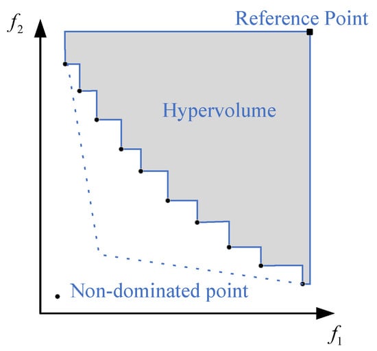
Figure 3. Schematic diagram of HV indicators in two-dimensional space.

4.3.2. Performance Profile Based on Hypervolume

To evaluate and compare the performance of different algorithms, a performance profile [9] based on the HV metric over the entire set of benchmark problems is employed. For a given test problem $\kappa \in \mathcal{K}$ and an algorithm $a_g\in \mathcal{A}g$, let $I_{\mathrm{HV}}^R={\displaystyle \frac{1}{I_{\mathrm{HV}}(\kappa ,a_g)}}$ be the reciprocal of the HV value, since a larger HV value indicates better algorithm performance. The performance profile of algorithm $a_g$ is then defined as the fraction of problems whose performance ratio ${\pi }_{\kappa ,a_g}$ is within a given threshold $\tau$, as expressed in Equation (17):

$${\rho }_{a_g}\left(\tau \right)={\displaystyle \frac{\mathrm{card}\{{\pi }_{\kappa ,a_g}\le \tau |\kappa \in \mathcal{K},a_g\in {\mathcal{A}}_g\}}{\mathrm{card}\left(\mathcal{K}\right)}}$$

(17)

where ${\pi }_{\kappa ,a_g}={\displaystyle \frac{I_{\mathrm{HV}}^R}{\min \left\{I_{\mathrm{HV}}^R\right|\kappa \in \mathcal{K},a_g\in {\mathcal{A}}_g\}}}$. Note that ${\pi }_{\kappa ,a_g}={\pi }_M$ if and only if algorithm $a_g$ fails to solve problem $\kappa$ satisfactorily, where ${\pi }_M\ge max\left\{{\pi }_{\kappa ,a_g}\right|\kappa \in \mathcal{K},a_g\in {\mathcal{A}}_g\}$.

4.4. Results and Discussion

4.4.1. Performance Analysis Based on HV

Table 3, Figure 4 and Figure 5 collectively demonstrate distinct performance differences among the compared algorithms on both the ZDT and WFG benchmark sets. In Table 3, the best algorithm is labeled with a darker gray background and the second best algorithm with a lighter gray background. Additionally, to determine whether there are statistically significant differences among all tested algorithms when solving different benchmark problems, Table 4 presents the results of the two-sided Wilcoxon rank-sum test [35] on the HV metric across all algorithms. A significance level of 0.05 is adopted. In the table, “+” indicates that the algorithm in the corresponding row is statistically significantly better than the algorithm in the corresponding column for a given problem; “-” means that the algorithm in the corresponding column is statistically significantly better than the one in the row; and “=” denotes no statistically significant difference between the two compared algorithms.

Table 3. Statistical results of HV obtained by the compared algorithms.

Problem	Algorithm
	DMSCFSM	DMS	MultiGlods	BoostDMS	MOIF	NSGA-II	MOEA/D
ZDT1	$0.664$	$0.268$	$0.663$	$0.618$	$0.664$	$0.636$	$0.215$
	$\left(0.00\right)$	$\left(0.00\right)$	$\left(0.00\right)$	$\left(0.00\right)$	$\left(0.00\right)$	$\left(0.01\right)$	$\left(0.09\right)$
ZDT2	$0.331$	$0.080$	$0.330$	$0.331$	$0.330$	$0.216$	$0.002$
	$\left(0.00\right)$	$\left(0.00\right)$	$\left(0.00\right)$	$\left(0.00\right)$	$\left(0.00\right)$	$\left(0.09\right)$	$\left(0.01\right)$
ZDT3	$0.448$	$0.260$	$0.464$	$0.448$	$0.383$	$0.496$	$0.105$
	$\left(0.00\right)$	$\left(0.00\right)$	$\left(0.00\right)$	$\left(0.00\right)$	$\left(0.00\right)$	$\left(0.01\right)$	$\left(0.04\right)$
ZDT4	$0.595$	$0.332$	$0.665$	$0.499$	$0.000$	$0.118$	$0.007$
	$\left(0.00\right)$	$\left(0.00\right)$	$\left(0.00\right)$	$\left(0.00\right)$	$\left(0.00\right)$	$\left(0.13\right)$	$\left(0.03\right)$
ZDT6	$0.400$	$0.000$	$0.351$	$0.400$	$0.399$	$0.163$	$0.233$
	$\left(0.00\right)$	$\left(0.00\right)$	$\left(0.00\right)$	$\left(0.00\right)$	$\left(0.00\right)$	$\left(0.03\right)$	$\left(0.12\right)$
WFG1	$0.275$	$0.000$	$0.224$	$0.281$	$0.000$	$0.332$	$0.247$
	$\left(0.00\right)$	$\left(0.00\right)$	$\left(0.00\right)$	$\left(0.00\right)$	$\left(0.00\right)$	$\left(0.07\right)$	$\left(0.00\right)$
WFG2	$0.898$	$0.446$	$0.847$	$0.908$	$0.460$	$0.842$	$0.882$
	$\left(0.00\right)$	$\left(0.00\right)$	$\left(0.00\right)$	$\left(0.00\right)$	$\left(0.00\right)$	$\left(0.06\right)$	$\left(0.00\right)$
WFG3	$0.297$	$0.211$	$0.216$	$0.310$	$0.290$	$0.308$	$0.301$
	$\left(0.00\right)$	$\left(0.00\right)$	$\left(0.00\right)$	$\left(0.00\right)$	$\left(0.00\right)$	$\left(0.00\right)$	$\left(0.01\right)$
WFG4	$0.360$	$0.272$	$0.325$	$0.361$	$0.316$	$0.349$	$0.319$
	$\left(0.00\right)$	$\left(0.00\right)$	$\left(0.00\right)$	$\left(0.00\right)$	$\left(0.00\right)$	$\left(0.01\right)$	$\left(0.01\right)$
WFG5	$0.397$	$0.348$	$0.295$	$0.374$	$0.320$	$0.333$	$0.318$
	$\left(0.00\right)$	$\left(0.00\right)$	$\left(0.00\right)$	$\left(0.00\right)$	$\left(0.00\right)$	$\left(0.01\right)$	$\left(0.00\right)$
WFG6	$0.415$	$0.376$	$0.381$	$0.393$	$0.359$	$0.331$	$0.336$
	$\left(0.00\right)$	$\left(0.00\right)$	$\left(0.00\right)$	$\left(0.00\right)$	$\left(0.00\right)$	$\left(0.02\right)$	$\left(0.01\right)$
WFG7	$0.368$	$0.350$	$0.300$	$0.365$	$0.337$	$0.355$	$0.338$
	$\left(0.00\right)$	$\left(0.00\right)$	$\left(0.00\right)$	$\left(0.00\right)$	$\left(0.00\right)$	$\left(0.01\right)$	$\left(0.01\right)$
WFG8	$0.213$	$0.261$	$0.221$	$0.189$	$0.256$	$0.258$	$0.234$
	$\left(0.00\right)$	$\left(0.00\right)$	$\left(0.00\right)$	$\left(0.00\right)$	$\left(0.00\right)$	$\left(0.04\right)$	$\left(0.04\right)$
WFG9	$0.331$	$0.321$	$0.388$	$0.323$	$0.288$	$0.340$	$0.336$
	$\left(0.00\right)$	$\left(0.00\right)$	$\left(0.00\right)$	$\left(0.00\right)$	$\left(0.00\right)$	$\left(0.01\right)$	$\left(0.00\right)$

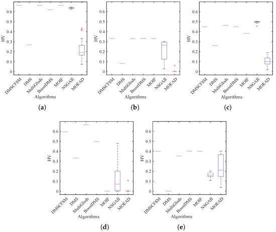
Figure 4. HV boxplots for ZDT benchmark set. (a) ZDT1; (b) ZDT2; (c) ZDT3; (d) ZDT4; (e) ZDT6.

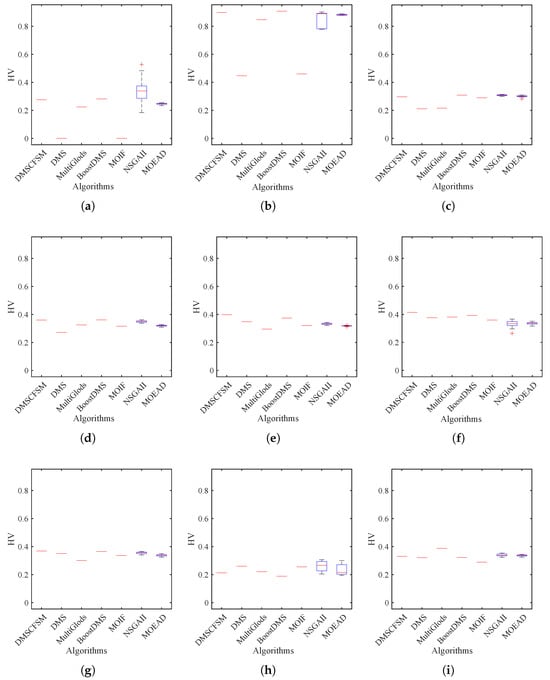
Figure 5. HV boxplots for WFG benchmark set. (a) WFG1; (b) WFG2; (c) WFG3; (d) WFG4; (e) WFG5; (f) WFG6; (g) WFG7; (h) WFG8; (i) WFG9.

Table 4. Results of Wilcoxon rank-sum test of $I_{\mathrm{HV}}$.

Algorithm	Compared Algorithm
	DMS	MultiGlods	BoostDMS	MOIF	NSGA-II	MOEA/D
DMSCFSM	+ + + + + + + + + + + + - +	+ +- - + + + + + + + + - -	+ - - + - - - - - + + + + +	+ + + + + + + + + + + + - +	+ + - + + - + - + + + + - -	+ + + + + + + - + + + + = -
DMS	—	- - - - - - - - - + - + + -	- - - - - - - - - - - - + -	- - - + - = - - - + + + + +	- - - + - - - - - + + - = -	+ + + + - - - - - + + + + -
MultiGlods	—	—	+ - + +- - - - - - - - + +	- - + + - + + - + - + - - +	+ + - + + - = - - - + - - +	+ + + + + - - - + - + - = +
BoostDMS	—	—	—	- + + + + + + + + + + + - +	- + - + + - + + + + + + - -	+ + + + + + + + + + + + - -
MOIF	—	—	—	—	+ + - - + - - - - - + - = -	+ + + + + - - - - + + - + -
NSGA-II	—	—	—	—	—	+ + + + - + = + + + = + + =

Table 3 and Table 4 and Figure 4 demonstrate that the proposed DMSCFSM method exhibits a clear advantage in solving ZDT problems (with the exception of ZDT3), which may be attributed to the discontinuous nature of ZDT3’s Pareto front. In contrast, both NSGA-II and MultiGlods show superior performance in solving ZDT3, which can be linked to their enhanced global search capabilities. When examining solution stability across DMSCFSM, DMS, MultiGlods, BoostDMS, MOIF, and the population-based algorithms NSGA-II and MOEA/D, the former group shows significantly lower variability. Specifically, their standard deviations remain at $0.00$ throughout all the benchmark problems, indicating superior stability compared to NSGA-II and MOEA/D.

Through comparative analysis of DMSCFSM, BoostDMS, and DMS, it can be observed that BoostDMS demonstrates clear superiority over DMS. This indicates that incorporating the search step design into the DMS framework significantly enhances the algorithm’s performance. Although DMSCFSM substantially outperforms DMS, it surpasses BoostDMS only on ZDT1 and ZDT4 problems. These findings collectively indicate that integrating search steps improves algorithmic performance. Furthermore, DMS-based methods with search steps require fewer function evaluations to achieve high-quality Pareto fronts. However, the incorporation of the search step increases the algorithm’s computational time in some cases. As a result, both DMSCFSM and BoostDMS show particular advantages for expensive MOO problems where function evaluations are computationally costly. In contrast, for problems with inexpensive objective functions, the additional computational cost introduced by search steps may not be justified by the performance gains.

On the WFG benchmark set, Table 3 and Table 4 and Figure 5 collectively demonstrate that DMSCFSM achieves the best performance among all compared algorithms. Except WFG8, DMSCFSM outperforms both DMS and MOIF across the WFG benchmark set. Specifically, it surpasses MultiGlods on seven out of nine problems, exceeds MOEA/D on six problems, and outperforms both BoostDMS and NSGA-II on five problems. The stability analysis of DMSCFSM, DMS, MultiGlods, BoostDMS, MOIF, and the population-based algorithms NSGA-II and MOEA/D yields results consistent with those from the ZDT benchmark problems, demonstrating that algorithms derived from single-objective mathematical optimization methods exhibit significantly better stability than population-based approaches.

The comparison among DMS, BoostDMS, and DMSCFSM similarly demonstrates that BoostDMS, enhanced with surrogate models, exhibits improved robustness and effectiveness over the basic DMS framework. Furthermore, DMSCFSM significantly outperforms BoostDMS on a larger number of benchmark problems, highlighting the efficacy of the proposed improvements.

Based on the Wilcoxon test results in Table 4, DMSCFSM shows no statistically significant difference from MOEA/D only on the WFG8 problem, while exhibiting significant differences in all other benchmark problems. Specifically, DMSCFSM significantly outperforms other algorithms in 64 out of 84 comparisons and surpasses BoostDMS in 62 scenarios, implying the superiority of the proposed method.

However, compared to BoostDMS, DMSCFSM incurs additional computational costs due to the incorporation of a Pareto dominance-based comparison function. Nonetheless, this function enables the algorithm to systematically leverage the dominance strength of solutions to efficiently filter out non-dominated solutions that are likely to be dominated later. This approach reduces the number of Pareto dominance comparisons (as implemented in Lines 9–24 of Algorithm 2) required in subsequent iterations. Moreover, the introduced sparse modeling technique helps mitigate the curse of dimensionality and enhances the generalization ability of the surrogate models. Consequently, DMSCFSM achieves superior performance compared to other algorithms under the same function evaluation budget. In particular, for expensive MOO problems, such as those involving simulation-based objectives, the computational time required for the comparison function becomes negligible compared to the cost of each objective function evaluation. This makes DMSCFSM especially advantageous for problems with computationally intensive objectives. Therefore, it is essential to balance the computational overhead of the comparison process against the cost of objective function evaluations when selecting an approach.

4.4.2. Performance Analysis Based on Performance Profile

To effectively visualize and compare algorithm performance across a diverse set of problems, performance profiles are employed. Figure 6 presents the performance profiles plotted on a log scale for the performance ratio. The height of each curve at $\tau =0$ represents the proportion of problems where the corresponding algorithm achieves the best performance among all compared algorithms. These profiles are constructed based on the HV metric, evaluating seven algorithms (DMSCFSM, DMS, BoostDMS, MultiGlods, MOIF, NSGA-II, and MOEA/D) across the comprehensive benchmark set.

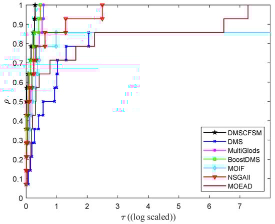
Figure 6. Comparing algorithms based on performance profiles.

As observed in Figure 6, the DMSCFSM algorithm achieves the highest efficiency, demonstrating the best performance at $\tau =0$ on the log scale, while maintaining robustness comparable to that of BoostDMS. Its performance profile shows the fastest initial convergence at small $\tau$ values and eventually reaches the maximum height, indicating DMSCFSM’s effectiveness in solving most benchmark problems under the given experimental setup. BoostDMS ranks second in performance, while MultiGlods also displays a rapidly ascending curve and high final attainment level, demonstrating considerable problem-solving capability. In contrast, NSGA-II, MOIF, MOEA/D, and DMS exhibit relatively weaker performance, requiring substantially larger $\tau$ thresholds to reach comparable solution proportions.

5. Conclusions

Multi-objective DFO plays a significant role in real-world applications, as the accurate resolution of such problems provides crucial support for decision-making processes. However, in many practical optimization scenarios, particularly those involving computationally expensive simulations, objective function evaluations tend to be extremely time-consuming. This underscores the importance of obtaining high-quality Pareto fronts with limited function evaluations.

This article presents a novel multi-objective DFO method developed within the DMS framework. The proposed algorithm incorporates two key improvements. The first is the application of a sparse modeling technique for surrogate model construction. The second is the implementation of a Pareto dominance-based comparison function to fully utilize non-dominated solution information. To assess algorithmic performance, comprehensive comparisons were conducted with six state-of-the-art algorithms using ZDT and WFG benchmark problems. Numerical experiments demonstrate that the proposed method achieves high-quality Pareto fronts with competitive performance and efficiency. However, the incorporation of comparison functions introduces additional computational costs, which may limit the algorithm’s applicability in certain scenarios. To assess the practical impact of this limitation, future work is required to evaluate its performance on more complex, high-dimensional problems and real-world engineering problems that are computationally expensive. Additionally, the algorithm’s performance is influenced by several parameters, such as the step-size update parameters ($\beta$ and $\gamma$) and the tolerance ($\epsilon$). Therefore, future research will also focus on enhancing the algorithm’s adaptive capabilities to reduce this dependency on manual parameter tuning.

References

- Custódio, A.L.; Madeira, J.F.A.; Vaz, A.I.F.; Vicente, L.N. Direct multisearch for multiobjective optimization. SIAM J. Optim. 2011, 21, 1109–1140. [Google Scholar] [CrossRef]
- Custodio, A.L.; Madeira, J.F.A. MultiGLODS: Global and local multiobjective optimization using direct search. J. Glob. Optim. 2018, 72, 323–345. [Google Scholar] [CrossRef]
- Jean Bigeon, S.L.D.; Salomon, L. DMulti-MADS: Mesh adaptive direct multisearch for bound-constrained blackbox multiobjective optimization. Comput. Optim. Appl. 2021, 79, 301–338. [Google Scholar] [CrossRef]
- Sander Dedoncker, W.D.; Naets, F. An adaptive direct multisearch method for black-box multi-objective optimization. Optim. Eng. 2022, 23, 1411–1437. [Google Scholar] [CrossRef]
- Berkemeier, M.; Peitz, S. Derivative-free multiobjective trust region descent method using radial basis function surrogate models. Math. Comput. Appl. 2021, 26, 31. [Google Scholar] [CrossRef]
- Liu, H.; Zhou, C.; Liu, F.; Duan, Z.; Zhao, H. A trust-region-like algorithm for expensive multi-objective optimization. Appl. Soft Comput. 2023, 148, 110892. [Google Scholar] [CrossRef]
- Mohammadi, A.; Hajinezhad, D.; Garcia, A. A trust-region approach for computing Pareto fronts in multiobjective derivative-free optimization. Optim. Lett. 2024, 19, 233–266. [Google Scholar] [CrossRef]
- Bisui, N.K.; Panda, G. A trust-region scheme for constrained multi-objective optimization problems with superlinear convergence property. Optim. Methods Softw. 2025, 40, 24–64. [Google Scholar] [CrossRef]
- Deb, K.; Pratap, A.; Agarwal, S.; Meyarivan, T. A fast and elitist multiobjective genetic algorithm: NSGA-II. IEEE Trans. Evol. Comput. 2002, 6, 182–197. [Google Scholar] [CrossRef]
- Zhang, Q.; Li, H. MOEA/D: A multiobjective evolutionary algorithm based on decomposition. IEEE Trans. Evol. Comput. 2007, 11, 712–731. [Google Scholar] [CrossRef]
- Stewart, R.H.; Palmer, T.S.; DuPont, B. A survey of multi-objective optimization methods and their applications for nuclear scientists and engineers. IEEE Trans. Syst. Man Cybern. Syst. 2021, 138, 103830. [Google Scholar] [CrossRef]
- Liu, Y.; Ding, J.; Li, Q.; Li, F.; Liu, J. A two-level model management-based surrogate-assisted evolutionary algorithm for medium-scale expensive multiobjective optimization. IEEE Trans. Syst. Man Cybern. Syst. 2025, 55, 8166–8180. [Google Scholar] [CrossRef]
- Si, L.; Zhang, X.; Tian, Y.; Yang, S.; Zhang, L.; Jin, Y. Linear subspace surrogate modeling for large-scale expensive single/multiobjective optimization. IEEE Trans. Evol. Comput. 2025, 29, 697–710. [Google Scholar] [CrossRef]
- Liu, J.; Liu, T. A two-stage multi-objective optimization algorithm for solving large-scale optimization problems. Algorithms 2025, 18, 164. [Google Scholar] [CrossRef]
- Audet, C.; Savard, G.; Zghal, W. Multiobjective optimization through a series of single-objective formulations. SIAM J. Optim. 2008, 19, 188–210. [Google Scholar] [CrossRef]
- Ryu, J.h.; Kim, S. A derivative-free trust-region method for biobjective optimization. SIAM J. Optim. 2014, 24, 334–362. [Google Scholar] [CrossRef]
- Thomann, J.; Eichfelder, G. A trust-region algorithm for heterogeneous multiobjective optimization. SIAM J. Optim. 2019, 29, 1017–1047. [Google Scholar] [CrossRef]
- Torczon, V. On the convergence of pattern search algorithms. SIAM J. Optim. 1997, 7, 1–25. [Google Scholar] [CrossRef]
- Audet, C.; Dennis, J.E. Mesh adaptive direct search algorithms for constrained optimization. SIAM J. Optim. 2006, 17, 188–217. [Google Scholar] [CrossRef]
- Audet, C.; Savard, G.; Zghal, W. A mesh adaptive direct search algorithm for multiobjective optimization. Eur. J. Oper. Res. 2010, 204, 545–556. [Google Scholar] [CrossRef]
- Brás, C.P.; Custódio, A.L. On the use of polynomial models in multiobjective directional direct search. Comput. Optim. Appl. 2020, 77, 897–918. [Google Scholar] [CrossRef]
- Tavares, S.; Brás, C.P.; Custódio, A.L.; Duarte, V.; Medeiros, P. Parallel strategies for direct multisearch. Numer. Algorithms 2023, 92, 1757–1788. [Google Scholar] [CrossRef]
- Liuzzi, G.; Lucidi, S.; Rinaldi, F. A derivative-free approach to constrained multiobjective nonsmooth optimization. SIAM J. Optim. 2016, 26, 2744–2774. [Google Scholar] [CrossRef]
- Silva, E.J.; Custódio, A.L. An inexact restoration direct multisearch filter approach to multiobjective constrained derivative-free optimization. Optim. Methods Softw. 2025, 40, 406–432. [Google Scholar] [CrossRef]
- Powell, M.J.D. Developments of NEWUOA for minimization without derivatives. IMA J. Numer. Anal. 2008, 28, 649–664. [Google Scholar] [CrossRef]
- Dejemeppe, C.; Schaus, P.; Deville, Y. Derivative-free optimization: Lifting single-objective to multi-objective algorithm. In Proceedings of the Integration of AI and OR Techniques in Constraint Programming, Barcelona, Spain, 18–22 May 2015; Michel, L., Ed.; Springer: Cham, Switzerland, 2015; pp. 124–140. [Google Scholar] [CrossRef]
- Davis, C. Theory of positive linear dependence. Am. J. Math. 1954, 76, 733–746. [Google Scholar] [CrossRef]
- Candes, E.; Tao, T. The Dantzig selector: Statistical estimation when p is much larger than n. Ann. Stat. 2007, 35, 2313–2351. [Google Scholar] [CrossRef]
- Mazumder, R.; Choudhury, A.; Iyengar, G.; Sen, B. A computational framework for multivariate convex regression and its variants. J. Am. Stat. Assoc. 2019, 114, 318–331. [Google Scholar] [CrossRef]
- Chen, S.S.; Donoho, D.L.; Saunders, M.A. Atomic decomposition by basis pursuit. SIAM J. Sci. Comput. 1998, 20, 33–61. [Google Scholar] [CrossRef]
- Cocchi, G.; Liuzzi, G.; Papini, A.; Sciandrone, M. An implicit filtering algorithm for derivative-free multiobjective optimization with box constraints. Comput. Optim. Appl. 2018, 69, 267–296. [Google Scholar] [CrossRef]
- Durillo, J.J.; Nebro, A.J. jMetal: A Java framework for multi-objective optimization. Adv. Eng. Softw. 2011, 42, 760–771. [Google Scholar] [CrossRef]
- Huband, S.; Barone, L.; While, L.; Hingston, P. A scalable multi-objective test problem toolkit. In Proceedings of the Evolutionary Multi-Criterion Optimization, Guanajuato, Mexico, 9–11 March 2005; Coello Coello, C.A., Hernández Aguirre, A., Zitzler, E., Eds.; Springer: Berlin/Heidelberg, Germany, 2005; pp. 280–295. [Google Scholar] [CrossRef]
- Zitzler, E.; Thiele, L. Multiobjective evolutionary algorithms: A comparative case study and the strength Pareto approach. IEEE Trans. Evol. Comput. 1999, 3, 257–271. [Google Scholar] [CrossRef]
- Haynes, W. Wilcoxon rank sum test. In Encyclopedia of Systems Biology; Dubitzky, W., Wolkenhauer, O., Cho, K.H., Yokota, H., Eds.; Springer: New York, NY, USA, 2013; pp. 2354–2355. [Google Scholar] [CrossRef]
Disclaimer/Publisher’s Note: The statements, opinions and data contained in all publications are solely those of the individual author(s) and contributor(s) and not of MDPI and/or the editor(s). MDPI and/or the editor(s) disclaim responsibility for any injury to people or property resulting from any ideas, methods, instructions or products referred to in the content. |
© 2025 by the authors. Licensee MDPI, Basel, Switzerland. This article is an open access article distributed under the terms and conditions of the Creative Commons Attribution (CC BY) license (https://creativecommons.org/licenses/by/4.0/).