Hypersphere-Guided Reciprocal Point Learning for Open-Set Industrial Process Fault Diagnosis

Abstract

Deep neural networks (DNNs) have achieved superior performance in diagnosing process faults, but they lack robustness when encountering novel fault types absent from training sets. Such unknown faults commonly appear in industrial settings, and conventional DNNs often misclassify them as one of the known fault types. To address this limitation, we formulate the concept of open-set fault diagnosis (OSFD), which seeks to distinguish unknown faults from known ones while correctly classifying the known faults. The primary challenge in OSFD lies in minimizing both the empirical classification risk associated with known faults and the open space risk without access to training data for unknown faults. In order to mitigate these risks, we introduce a novel approach called hypersphere-guided reciprocal point learning (SRPL). Specifically, SRPL preserves a DNN for feature extraction while constraining features to lie on a unit hypersphere. To reduce empirical classification risk, it applies an angular-margin penalty that explicitly increases intra-class compactness and inter-class separation for known faults on the hypersphere, thereby improving discriminability among known faults. Additionally, SRPL introduces reciprocal points on the hypersphere, with each point acting as a classifier by occupying the extra-class region associated with a particular known fault. The interactions among multiple reciprocal points, together with the deliberate synthesis of unknown fault features on the hypersphere, serve to lower open-space risk: the reciprocal-point interactions provide an indirect estimate of unknowns, and the synthesized unknowns provide a direct estimate, both of which enhance distinguishability between known and unknown faults. Extensive experimental results on the Tennessee Eastman process confirm the superiority of the proposed method compared to state-of-the-art OSR algorithms, e.g., an 82.32% AUROC score and a 71.50% OSFDR score.

1. Introduction

Data-driven process monitoring [1,2] is increasingly essential for maintaining the safety and stability of informatized industrial systems, encompassing two primary tasks: fault detection and fault diagnosis. Over recent decades, numerous one-class classifiers trained only on normal data—particularly deep neural network (DNN) models [3,4]—have demonstrated superior performance in fault detection. More recently, attention has shifted to the next fault diagnosis task, where DNN-based multi-class classifiers are being actively developed [5,6]. Its performance, however, depends strongly on the presence and quality of labeled fault samples in the training set. Because collecting labeled fault data is difficult, researchers have proposed methods to bolster the robustness of DNN-based fault diagnosis from several angles. Data-generation approaches use digital twins [7], generative adversarial networks [8,9], or metric learning [10] to synthesize virtual samples and augment training sets. Transfer learning methods train models on source-domain data and adapt them for deployment in target domains [11]. Semi-supervised approaches leverage unlabeled samples effectively [12,13]. Imbalanced learning techniques aim to balance fault diagnosis performance across minor and major classes [14].

Despite progress with DNN-based fault diagnosis models in mitigating the scarcity of sample-label pairs in training sets, they remain vulnerable to novel fault types. When a test sample represents a fault not included in the training set—an unknown fault—the models typically misclassify it as one of the known fault types. This failure stems from the closed-set assumption that the training data encompass all possible fault types. In practice, dynamic production environments and the low occurrence frequency of some faults make encounters with unknown faults likely. Therefore, we argue that a robust fault diagnosis approach must both distinguish unknown faults from known ones and correctly classify known faults; we refer to this combined objective as open-set fault diagnosis (OSFD) in this paper.

To our knowledge, few studies have addressed the OSFD task using DNNs. Rodríguez-Ramos et al. [15] recently proposed an event-detection method based on the local outlier factor algorithm in Processes, but that approach remains constrained by the limitations of traditional machine learning. Given this context, we briefly review recent work that explicitly considers the open-set nature of testing datasets. Yu et al. [16] and Wang et al. [17] each proposed incremental-learning fault-diagnosis models that assume unknown faults appear gradually; however, these studies emphasize incorporating detected unknown faults into closed-set diagnosis systems rather than on identifying unknown faults. Zhuo and Ge [18] proposed an any-shot learning fault-diagnosis model in which fault attributes serve as side information to guide a generative adversarial network (GAN) to synthesize samples of minor classes or unknown faults. Yet many industrial processes lack accurate fault attributes for all fault types, so synthesized unknown-fault samples for training OSFD models cannot be guaranteed. In summary, developing a new DNN-based model specifically for the OSFD task remains necessary.

In computer vision domains such as autonomous driving and medical image analysis, an analogous task called open-set recognition (OSR) [19,20] has been widely studied. OSR aims to detect unknown classes while preserving classification performance on known classes. Typical DNN-based OSR methods, including OpenMax [21] and prototype learning [22], assume that unknown-class examples lie farther from each known-class “prototype” than known-class examples do in deep embedding spaces. Modeling distances between samples and prototypes therefore supports both classification of known classes and detection of unknown classes. In addition to these discriminative approaches, generative models such as autoencoders (AEs) [23,24] and GANs [25] have been combined with classifiers to shape embedding spaces for unknown-class detection. Although these post-processing OSR methods empirically extend closed-set models to open-set settings, they focus primarily on enhancing discriminative features for known classes and ignore the distribution of unknown classes during training, which reduces their ability to separate known and unknown classes.

Among DNN-based open-set recognition (OSR) methods, reciprocal point learning (RPL) [26,27] is particularly well suited for OSFD. In RPL, each reciprocal point represents the extra-class region of a corresponding known class in the deep embedding space. By interacting multiple reciprocal points, RPL can estimate the distribution of unknown classes without access to unknown-class training samples. However, directly applying RPL to OSFD still yields high empirical classification risk on known faults and potential open-space risk for unknown faults, because many faults exhibit similar operating conditions. To address these challenges, we propose hyperSphere–guided RPL (SRPL), which adapts OSR-oriented RPL for the OSFD setting. Specifically, SRPL keeps a backbone network for feature extraction but constrains the features to lie on a unit hypersphere as the deep embedding space. On this hypersphere, SRPL employs a set of reciprocal points, each acting as the classifier for a specific known fault. To reduce empirical classification risk, we introduce a Quadratic Subtractive Angular Margin (QSAM) penalty defined on the hypersphere. QSAM explicitly increases intra-class compactness and inter-class separation of known faults, which is particularly beneficial when discriminating between similar faults. To lower open-space risk, we porpose Normal State Information (NSI) aided manifold mixup on the hypersphere. NSI-aided manifold mixup randomly interpolates abnormal-state variations as training samples, while reciprocal points provide an implicit representation of extra-class regions. Together, NSI-aided manifold mixup and reciprocal points estimate unknown-fault distributions more effectively and thereby enhance the distinguishability between known and unknown faults. Figure 1 shows these modules of the proposed SPRL algorithm. We evaluate SRPL on the Tennessee–Eastman process. The results show that SRPL attains superior OSFD performance compared with state-of-the-art OSR methods. The main contributions of this paper are threefold as follows.

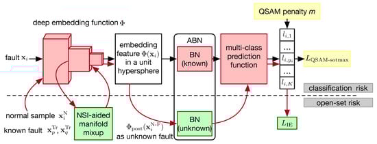
Figure 1. An overview of the proposed SRPL algorithm. The deep embedding function $\Phi$ is modeled by a backbone network that maps faults detected by the upstream fault detection task onto an embedding feature residing on the unit hypersphere. The multi-class prediction function $\Psi$ implemented through a fully-connected neural network, takes this embedding feature as input and generates its corresponding label as output. Once the models $\Phi$ and $\Psi$ are trained, the largest logit serves as the score for unknown fault detection. This approach incorporates two key concepts: the QSAM penalty, which reduces empirical classification risk, and NSI-aided manifold mixup, which addresses open-set risks. We present these two concepts and the training procedure including a FT step in Section 3.

• We formalized the OSFD task as an alternative to the conventional closed-set formulation and proposed SRPL, an RPL-solution grounded in lower lowerer empirical classification risk and open-space risk.
• We introduced QSAM on the hypersphere to explicitly increase intra-class compactness and inter-class separation for known faults, thereby producing more discriminative features and reducing the space inadvertently allocated to known faults.
• We enabled OSFD to leverage normal-state training data as side information via NSI-aided manifold mixup. NSI-aided manifold mixup can synthesize unknown faults simply and effectively, and these synthesized examples are used to directly constrain the size of the open space defined by reciprocal points.

2. Related Works

We review two related classification frameworks based on DNNs: softmax loss and RPL. Considering given a DNN-based classifier $f:{\mathbb{R}}^D\mapsto \{1,\dots K\}$ that is disentangled into two parts.

• A deep embedding function $\Phi :{\mathbb{R}}^D\mapsto {\mathbb{R}}^d$ with parameters $\mathbf{\Theta }$, where D and d are the dimension of the input ${\mathbf{x}}_i$ and its embedding feature $\Phi \left({\mathbf{x}}_i\right)$, respectively.
• A measurable multi-class prediction function $\Psi :{\mathbb{R}}^d\to {\mathbb{R}}^K$ with weights $\mathbf{W}=[{\mathbf{w}}_1,{\mathbf{w}}_2,\dots ,{\mathbf{w}}_K]\in {\mathbb{R}}^{d\times K}$, where K denotes the number of known classes.

2.1. Softmax Loss

In a DNN-based classifier f, $\Psi$ is typically realized by the final fully connected layer. The output logit for known class k is $l_{i,k}=\Phi {\left({\mathbf{x}}_i\right)}^{\mathrm{T}}{\mathbf{w}}_k$. The softmax function then converts $l_{i,k}$ into class probabilities by $p(y=k\mid {\mathbf{x}}_i)={\displaystyle \frac{exp\left(l_{i,k}\right)}{{\sum }_{j=1}^{K}exp\left(l_{i,j}\right)}}$. The predicted class for ${\mathbf{x}}_i$ is the one with the highest probability, i.e., ${\widehat{y}}_i={\arg \max }_{k}p(y=k\mid {\mathbf{x}}_i)$. Parameters $\mathbf{\Theta }$ and $\mathbf{W}$ are generally learned by minimizing the softmax loss, defined as the average negative log-probability of the correct label $y_i$ for each training sample $x_i$ as

$$L_{\mathrm{softmax}}=-{\displaystyle \frac{1}{N}}\sum _{i=1}^{N}log\left(p(y=y_i|{\mathbf{x}}_i)\right)=-{\displaystyle \frac{1}{N}}\sum _{i=1}^{N}log\left({\displaystyle \frac{exp\left(l_{i,y_i}\right)}{{\sum }_{j=1}^{K}exp\left(l_{i,j}\right)}}\right),$$

(1)

where N denotes the number of training samples. For the geometric interpretation of $L_{\mathrm{softmax}}$ in Equation (1), $l_{i,k}$ can be expressed as $l_{i,k}=\Phi {\left({\mathbf{x}}_i\right)}^{\mathrm{T}}{\mathbf{w}}_k=\parallel \Phi \left({\mathbf{x}}_i\right)\parallel \parallel {\mathbf{w}}_k\parallel cos{\theta }_{i,k}$, where ${\theta }_{i,k}\in [0,\pi ]$ denotes the angle between $\Phi \left({\mathbf{x}}_i\right)$ and ${\mathbf{w}}_k$. Thus, classification is determined by comparing the dot products between $\Phi \left({\mathbf{x}}_i\right)$ and each ${\mathbf{w}}_k$, illustrated in Figure 2a.

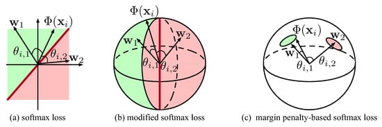
Figure 2. Geometric interpretation of a binary classification based on different softmax losses.

To further visualize $L_{\mathrm{softmax}}$, each $\Phi \left({\mathbf{x}}_i\right)$ and ${\mathbf{w}}_k$ can be re-scaled by ${\mathcal{l}}_2$ normalization as $\parallel \Phi \left({\mathbf{x}}_i\right)\parallel =1$ and $\parallel {\mathbf{w}}_k\parallel =1$ according to [28]. After this re-scaling, $\Phi \left({\mathbf{x}}_i\right)$ and ${\mathbf{w}}_k$ lie on a unit hypersphere, and the classifier depends solely on the angle distance ${\theta }_{i,k}$. As shown in Figure 2b, a small ${\theta }_{i,k}$ means $\Phi \left({\mathbf{x}}_i\right)$ lies closer to ${\mathbf{w}}_k$, which increases $l_{i,k}=cos{\theta }_{i,k}$ and therefore raises the probability that ${\mathbf{x}}_i$ will be assigned to known class k, i.e., ${\displaystyle \frac{exp\left(cos{\theta }_{i,k}\right)}{{\sum }_{j=1}^{K}exp\left(cos{\theta }_{i,j}\right)}}$. In other words, ${\mathbf{w}}_k$ serves as the center or prototype of known class k. The normalized form of $L_{\mathrm{softmax}}$ in Equation (1) yields the Modified softmax loss as

$$L_{\mathrm{M}-\mathrm{softmax}}=-{\displaystyle \frac{1}{N}}\sum _{i=1}^{N}log\left({\displaystyle \frac{exp\left(cos{\theta }_{i,y_i}\right)}{{\sum }_{j=1}^{K}exp\left(cos{\theta }_{i,j}\right)}}\right).$$

(2)

To improve discriminability among known classes, various variants of the $L_{\mathrm{M}-\mathrm{softmax}}$ function in Equation (2) have been developed for face verification. These variants integrate unique margin penalties into the target logit $l_{i{y}_i}=cos{\theta }_{i,y_i}$ [29,30], deliberately increasing the distance and decreasing the corresponding probability. For instance, ArcFace [29] introduces an angular margin m to increase ${\theta }_{i,y_i}$ as

$$l_{i{y}_i}=cos({\theta }_{i,y_i}+m).$$

(3)

This approach effectively increases intra-class compactness while simultaneously expanding inter-class separation, as demonstrated in Figure 2c.

2.2. Reciprocal Point Learning

In the DNN-based classifier f reviewed here, the final fully connected layer $\Psi$ is implemented by reciprocal point learning, wherein each ${\mathbf{w}}_k$ serves as a reciprocal point rather than a prototype. Each reciprocal point ${\mathbf{w}}_k$ represents the extra-class region associated with known class k in the deep embedding space. Consequently, samples of known class k should lie farther from ${\mathbf{w}}_k$ than samples of other known classes and unknown classes. In other words, a larger distance between $\Phi \left({\mathbf{x}}_i\right)$ and ${\mathbf{w}}_k$ raises the probability that ${\mathbf{x}}_i$ will be assigned to known class k. Therefore, the output logit for known class k is modeled as the negative dot product as $l_{i,k}=-\parallel \Phi \left({\mathbf{x}}_i\right)\parallel \parallel {\mathbf{w}}_k\parallel cos{\theta }_{i,k}$. The parameters $\mathbf{\Theta }$ and $\mathbf{W}$ can likewise be learned via $L_{\mathrm{softmax}}$ in Equation (1).

During training, RPL builds on $L_{\mathrm{softmax}}$ to increase the distance between each known class sample and its corresponding reciprocal point in the deep embedding space. The confrontation among multiple reciprocal points produces discriminative features for the known classes. Importantly, each known class occupies the extra-class region of other known classes. By interacting, the reciprocal points that represent the open space of unknown classes allow RPL to indirectly estimate the distribution of unknown classes without access to unknown-class training samples. As a result, known classes are pushed toward the periphery of the embedding space while unknown classes are constrained toward the interior.

3. Methodology

3.1. Problem Definition

Given a training dataset ${\mathcal{D}}_{\mathrm{Tr}}$, a testing dataset ${\mathcal{D}}_{\mathrm{Te}}$, and a normal dataset ${\mathcal{D}}_{\mathrm{N}}$ as

$$\begin{array}{cc}\hfill {\mathcal{D}}_{\mathrm{Tr}}& =\{({\mathbf{x}}_1^{\mathrm{Tr}},y_1^{\mathrm{Tr}}),\dots ,({\mathbf{x}}_{N_{\mathrm{Tr}}}^{\mathrm{Tr}},y_{N_{\mathrm{Tr}}}^{\mathrm{Tr}})\},y_i^{\mathrm{Tr}}\in \{1,\cdots ,K\},\hfill \end{array}$$

(4)

$$\begin{array}{cc}\hfill {\mathcal{D}}_{\mathrm{Te}}& =\{({\mathbf{x}}_1^{\mathrm{Te}},y_1^{\mathrm{Te}}),\dots ,({\mathbf{x}}_{N_{\mathrm{Te}}}^{\mathrm{Te}},y_{N_{\mathrm{Te}}}^{\mathrm{Te}})\},y_i^{\mathrm{Te}}\in \{1,\cdots ,K+U\},\hfill \end{array}$$

(5)

$$\begin{array}{cc}\hfill {\mathcal{D}}_{\mathrm{N}}& =\{{\mathbf{x}}_1^{\mathrm{N}},\dots ,{\mathbf{x}}_{N_{\mathrm{N}}}^{\mathrm{N}}\},\hfill \end{array}$$

(6)

where ${\mathcal{D}}_{\mathrm{Tr}}$ contains $N_{\mathrm{Tr}}$ fault samples with its label pairs $({\mathbf{x}}_i^{\mathrm{Tr}},y_i^{\mathrm{Tr}})$; ${\mathcal{D}}_{\mathrm{Te}}$ contains $N_{\mathrm{Te}}$ fault sample-label pairs $({\mathbf{x}}_i^{\mathrm{Te}},y_i^{\mathrm{Te}})$; ${\mathcal{D}}_{\mathrm{N}}$ contains $N_{\mathrm{N}}$ normal samples ${\mathbf{x}}_i^{\mathrm{N}}$; K and U denote the numbers of known and unknown fault types, respectively. For each known fault k, let ${\mathcal{S}}_k$ denote its deep embedding space, and ${\mathcal{O}}_k={\mathbb{R}}^d-{\mathcal{S}}_k$ denote its complementary extra-class (open) space. The open space ${\mathcal{O}}_k$ decomposes into two subspaces, i.e., ${\mathcal{O}}_k={\mathcal{S}}_{\ne k}\cup {\mathcal{O}}_{\mathrm{G}}$: ${\mathcal{S}}_{\ne k}$ denotes the intersection among the extra-class space of all other known faults, and ${\mathcal{O}}_{\mathrm{G}}={\cap }_{k=1}^K{\mathcal{O}}_k$ denotes the global open space of all unknown faults.

According to the definition of OSR [31], OSFD seeks to developing a DNN-based classifier f that minimizes the sum of the empirical classification risk ${\mathcal{R}}_{ϵ}$ for known faults and the open space risk $R_{\mathcal{O}}$ for unknown faults. The latter $R_{\mathcal{O}}$ represent the uncertainty associated with classifying unknown faults as known ones. This objective can be expressed mathematically as

$$\underset{f}{min}\{R_{ϵ}\left(f\right)+\xi R_{\mathcal{O}}\left(f\right)\},$$

(7)

where $\xi$ is a positive regularization parameter, which is calibrated to balance the fault diagnosis performance between known and unknown faults in accordance with the open-set degree in industrial settings. Within the deep embedding space, the multiclass prediction function $\Psi$ of the DNN-based classifier f can be decomposed into multiple binary-class prediction functions ${\psi }_k:{\mathbb{R}}^d\to \mathbb{R}$, such that $\Psi =\odot ({\psi }_1,\dots ,{\psi }_K)$, where ⊙ denotes an integration operation. Consequently, Equation (7) can be reformulated as

$$\underset{\Phi ,{\psi }_k}{min}\{\sum _{k=1}^K{R}_{ϵ}({\psi }_k,{\mathcal{S}}_k\cup {\mathcal{S}}_{\ne k})+\xi \sum _{k=1}^K{R}_{\mathcal{O}}({\psi }_k,{\mathcal{O}}_k)\}.$$

(8)

From a multiclass interaction perspective, the open space risk $R_{\mathcal{O}}$ in Equation (8) subsequently can be reformulated as

$$\sum _{k=1}^K{R}_{\mathcal{O}}({\psi }_k,{\mathcal{O}}_k)=R_{\mathcal{O}}(\Psi ,{\mathcal{O}}_{\mathrm{G}}).$$

(9)

It is important to note that quantitatively analyzing the open space risk $R_{\mathcal{O}}$ is often challenging, as unknown faults remain unrepresented during training.

Before introducing RPL into OSFD, we theoretically analyze its empirical classification risk $R_{ϵ}$ and open space risk $R_{\mathcal{O}}$.

• Each reciprocal point ${\mathbf{w}}_k$ serves as a binary-class prediction functions ${\psi }_k$. The empirical classification risk $R_{ϵ}$ in Equation (8) is typically optimized using the softmax loss on the training dataset ${\mathcal{D}}_{\mathrm{Tr}}$ as expressed in Equation (1). However, the similarity among various faults that deviate from the normal state with minor amplitude changes allows $R_{ϵ}$ to persist, resulting in inefficient diagnosis of known faults.
• Noted that, when optimizing the aforementioned $R_{ϵ}$, RPL facilitates maximizing the interval between each closed space ${\mathcal{S}}_k$ of known faults with its corresponding reciprocal point ${\mathbf{w}}_k$. Each reciprocal point ${\mathbf{w}}_k$ is associated with the open space ${\mathcal{O}}_{\mathrm{k}}$, and each known fault sample resides within the open space of other known faults, i.e., ${\mathcal{S}}_{\ne k}\in {\mathcal{O}}_k$. The approximation of open space risk $R_{\mathcal{O}}$ in Equation (8) thus can be simultaneously optimized through ${\mathcal{S}}_{\ne k}$, formulated as

  $$R_{\mathcal{O}}({\psi }_k,{\mathcal{O}}_k)\approx R_{\mathcal{O}}({\psi }_k,{\mathcal{S}}_{\ne k}).$$

  (10)
  As indicated in Equation (9), $R_{\mathcal{O}}$ fundamentally relies on the global open space ${\mathcal{O}}_{\mathrm{G}}$, which remains inaccessible during training in the absence of unknown faults. Consequently, while RPL indirectly reduces $R_{\mathcal{O}}$ as shown in Equation (10), it remains vulnerable to the identification of unknown faults that resemble known faults, unless ${\mathcal{O}}_{\mathrm{G}}$ is directly modeled.

To address the above two challenges, it is essential to further minimize both the empirical classification risk $R_{ϵ}$ in Equation (8) and the open space risk $R_{\mathcal{O}}$ in Equation (9) within the proposed SRPL framework. As illustrated in the graphical example in Figure 3, the central concept involves the implementation of a margin penalty m and the incorporation of manifold mixups within the unit hypersphere, as detailed below.

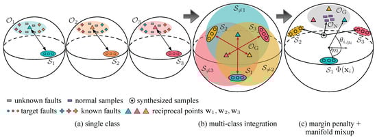
Figure 3. Geometric interpretation of SRPL with three types of known faults in the unit hypersphere: (a) the confrontation between each known faults and its corresponding reciprocal point, functioning as a binary classifier; (b) the confrontation among multiple reciprocal, which contract the global open space ${\mathcal{O}}_{\mathrm{G}}$; (c) QSAM-based softmax loss, aimed at enhancing intra-class compactness and inter-class separation of known faults, alongside NSI-aided manifold mixup for the synthesis of unknown faults.

3.2. Quadratic Subtractive Angular Margin Penalty

To further reduce the empirical classification risk $R_{ϵ}$ in Equation (8), we seek a deep embedding space characterized by greater intra-class compactness and inter-class separation of known faults. As noted in Section 2.1, both each reciprocal point ${\mathbf{w}}_k$ and each embedding feature $\Phi \left({\mathbf{x}}_i\right)$ are first ${\mathcal{l}}_2$ normalized, placing them on a unit hypersphere. Given the RPL property—where a larger distance between $\Phi \left({\mathbf{x}}_i\right)$ and ${\mathbf{w}}_k$ raises the probability that ${\mathbf{x}}_i$ will be assigned to known class k—the output logit for the k-th known fault produced by sample ${\mathbf{x}}_i$ is written as the negative dot product as

$$\begin{array}{cc}& \begin{array}{cc}{l}_{i,k}\hfill & =-\Phi {\left({\mathbf{x}}_i\right)}^{\mathrm{T}}{\mathbf{w}}_k\hfill \\ & =-\parallel \Phi \left({\mathbf{x}}_i\right)\parallel \parallel {\mathbf{w}}_k\parallel cos{\theta }_{i,k}\hfill \\ & =-cos{\theta }_{i,k}\hfill \end{array}\hfill \\ \mathrm{s}.\mathrm{t}.\hfill & \Phi \left({\mathbf{x}}_i\right)=\Phi \left({\mathbf{x}}_i\right)/\parallel \Phi \left({\mathbf{x}}_i\right)\parallel ,\hfill \\ & {\mathbf{w}}_k={\mathbf{w}}_k/\parallel {\mathbf{w}}_k\parallel .\hfill \end{array}$$

(11)

To obtain more discriminative features following Equation (3), we introduce an angular margin m by replacing the target logit $l_{i,y_i}=-cos{\theta }_{i,y_i}$ with $l_{i,y_i}=-cos({\theta }_{i,y_i}-m)$. This substitution deliberately decreases the target angle ${\theta }_{i,y_i}$ and the corresponding probability. Inspired by QAMFace that uses a target logit expressed as $l_{i,y_i}={(2\pi -({\theta }_{i,y_i}+m))}^2$ [30], we adopt a quadratic conversion function: $f\left(x\right)={(2\pi -x)}^2$ to map each target angle ${\theta }_{i,y_i}$ into a target logit $l_{i,y_i}={(2\pi -{\theta }_{i,k})}^2$, instead of using cosine. The resulting calibrated logits used for training are denoted as

$$l_{i,k}^{\mathrm{Cal}}=\left\{\begin{array}{cc}-{(2\pi -({\theta }_{i,k}-m))}^2\hfill & k=y_i\hfill \\ -{(2\pi -{\theta }_{i,k})}^2\hfill & k\ne y_i\hfill \end{array}\right..$$

(12)

Using this design, we define a Quadratic Subtractive Angular Margin (QSAM) based softmax loss denoted LQSAM-softmax as

$$\begin{array}{c}\hfill L_{\mathrm{QSAM}-\mathrm{softmax}}=-{\displaystyle \frac{1}{N}}{\sum }_{i=1}^{N}log\left({\displaystyle \frac{exp\left(l_{i,y_i}^{\mathrm{Cal}}\right)}{{\sum }_{j=1}^{K}exp\left(l_{i,j}^{\mathrm{Cal}}\right)}}\right).\end{array}$$

(13)

Noted that, the QSAM-based softmax loss differs from earlier margin-based losses in two respects: (1) it uses a quadratic mapping of ${\theta }_{i,y_i}$ to produce the logit rather than a cosine mapping, which yields a monotonic logit curve and a monotonic gradient that improve convergence, as discussed in [30]; and (2) the angular margin m is applied as a subtractive penalty rather than an additive one, lowering the target angle in accordance with the properties of reciprocal points.

Analysis of QSAM-based softmax loss. Equation (12) shows that the subtractive angular margin penalty m intentionally reduces the target angle distance, as illustrated in Figure 3c. Under this stricter condition, minimizing the QSAM-based softmax loss for known faults requires both compact intra-class distances and diverse inter-class distances. Consequently, the QSAM-based softmax loss in Equation (13) yields more discriminative features that enhance diagnosability of known faults, particularly similar ones, and it reduces over-allocated embedding space, thereby reserving more capacity to distinguish unknown from known faults.

Effects of Hypersphere Manifold. The unit hypersphere not only supports explicit optimization of embedding features but also enables more accurate estimation of the open space ${\mathcal{O}}_{\mathrm{k}}$ and the global one ${\mathcal{O}}_{\mathrm{G}}={\cap }_{k=1}^K{\mathcal{O}}_k$. As noted in Section 3.1, RPL can indirectly reduce the open space risk $R_{\mathcal{O}}$ by maximizing each interval between the closed space ${\mathcal{S}}_k$ and ${\mathcal{O}}_{\mathrm{k}}$, as shown in Equation (10). It is observed in [27] that an unbounded ${\mathcal{O}}_{\mathrm{G}}$ in infinite embedding space allows invaluable overlap with ${\mathcal{S}}_k$. In contrast, the unit hypersphere is finite, and the confrontation between multiple reciprocal points pushs each ${\mathcal{S}}_k$ and ${\mathcal{O}}_{\mathrm{G}}$ as far apart as possible. Consequently, the hypersphere manifold can further reduce $R_{\mathcal{O}}$ by limiting the size of ${\mathcal{O}}_{\mathrm{G}}$ on the finite unit hypersphere.

3.3. Normal State Information-Aided Manifold Mixup

To reduce the open space risk $R_{\mathcal{O}}$ as the manner in Equation (9), we seek to mimic the occurrence of novel faults and thereby directly minimize the global open space ${\mathcal{O}}_{\mathrm{G}}$. Note that, normal process data observed during upstream fault detection function as an unknown class for OSFD; consequently, the hypersphere corresponding to normal process data (denoted as ${\mathcal{O}}_{\mathrm{N}}$) is contained in the global open space ${\mathcal{O}}_{\mathrm{G}}$, i.e., ${\mathcal{O}}_{\mathrm{N}}\subset {\mathcal{O}}_{\mathrm{G}}$. Leveraging state information from available normal process data, we propose a simple yet effective method to synthesize unknown-fault samples with no additional time complexity: Normal State Information (NSI) aided manifold mixup.

We firstly decompose the embedding function $\Phi$ into the previous part ${\Phi }_{\mathrm{pre}}$ and the posterior one ${\Phi }_{\mathrm{post}}$, as

$$\Phi \left({\mathbf{x}}_i\right)={\Phi }_{\mathrm{post}}\left({\Phi }_{\mathrm{pre}}\left({\mathbf{x}}_i\right)\right),$$

(14)

where ${\Phi }_{\mathrm{pre}}\left({\mathbf{x}}_i\right)$ denotes the interior embedding feature of ${\mathbf{x}}_i$. Given two different type fault samples ${\mathbf{x}}_p^{\mathrm{Tr}}$ and ${\mathbf{x}}_q^{\mathrm{Tr}}$ from the training dataset ${\mathcal{D}}_{\mathrm{Tr}}$ ($y_p\ne y_q$) and a normal sample ${\mathbf{x}}_i^{\mathrm{N}}$ from the normal dataset ${\mathcal{D}}_{\mathrm{N}}$, NSI-aided manifold mixup is performed by two linear interpolations in the interior embedding space. First, mix two different type fault samples ${\mathbf{x}}_p^{\mathrm{Tr}}$ and ${\mathbf{x}}_q^{\mathrm{Tr}}$, yielding a manifold mixup ${\mathbf{x}}_i^{\mathrm{F}}$ as

$${\mathbf{x}}_i^{\mathrm{F}}={\gamma }_1·{\Phi }_{\mathrm{pre}}\left({\mathbf{x}}_p^{\mathrm{Tr}}\right)+(1-{\gamma }_1)·{\Phi }_{\mathrm{pre}}\left({\mathbf{x}}_q^{\mathrm{Tr}}\right).$$

(15)

Then, ${\mathbf{x}}_i^{\mathrm{N}-\mathrm{F}}$ is the manifold mixup between the normal sample ${\mathbf{x}}_i^{\mathrm{N}}$ with ${\mathbf{x}}_i^{\mathrm{F}}$ as

$${\mathbf{x}}_i^{\mathrm{N}-\mathrm{F}}={\gamma }_2·{\Phi }_{\mathrm{pre}}\left({\mathbf{x}}_i^{\mathrm{N}}\right)+(1-{\gamma }_2)·{\mathbf{x}}_i^{\mathrm{F}}.$$

(16)

Noted that, the mixing coefficients ${\gamma }_1,{\gamma }_2\in [0,1]$ are drawn randomly from a beta distribution as proposed in manifold mixup [32]. The generated mixup ${\mathbf{x}}_i^{\mathrm{N}-\mathrm{F}}$ finally passes through the posterior embedding function, yielding ${\Phi }_{\mathrm{post}}\left({\mathbf{x}}_i^{\mathrm{N}-\mathrm{F}}\right)$ lies on the hypersphere, as shown in Figure 3c. The detailed procedure for NSI-aided manifold mixup during training is given in Algorithm 1. For a mini-batch of size $N_{\mathrm{B}}$, we randomly shuffle the mini-batch in line 2 and perform NSI-aided manifold mixup on corresponding pairs from different fault types in line 9. Note that the size of mixup $N_{\mathrm{M}}$ is less than or equal to that of $N_{\mathrm{B}}$, and the order of magnitude of the forward and backward computational complexity in Equations (15) and (16) matches that of vanilla training.

Algorithm 1: The procedure of the NSI-aided manifold mixup during training.

Since the interpolation between two different known faults are often regions of low-confidence predictions for known faults [33] and ${\mathcal{O}}_{\mathrm{N}}\subset {\mathcal{O}}_{\mathrm{G}}$, we assume that ${\Phi }_{\mathrm{post}}\left({\mathbf{x}}_i^{\mathrm{N}-\mathrm{F}}\right)$ with high confidence to unknown faults. Subsequently, we treat ${\Phi }_{\mathrm{post}}\left({\mathbf{x}}_i^{\mathrm{N}-\mathrm{F}}\right)$ to estimate the distribution of the global open space ${\mathcal{O}}_{\mathrm{G}}$. We define this estimation by the information-entropy loss over each logit $l_{i,k}=-cos{\theta }_{i,k}$, formulated as

$$L_{\mathrm{IE}}=-{\displaystyle \frac{1}{N_{\mathrm{M}}}}\sum _{i=1}^{N_{\mathrm{M}}}({\displaystyle \frac{1}{K}}\sum _{k=1}^K{l}_{i,k}·\log \left(l_{i,k}\right)).$$

(17)

When all logit are equal—that is, when the angle distances between ${\Phi }_{\mathrm{post}}\left({\mathbf{x}}_i^{\mathrm{N}-\mathrm{F}}\right)$ and all reciprocal points are identical—$L_{\mathrm{IE}}$ attains its minimum. As illustrated in Figure 3c, employing ${\Phi }_{\mathrm{post}}\left({\mathbf{x}}_i^{\mathrm{N}-\mathrm{F}}\right)$ explicitly drives the global open space ${\mathcal{O}}_{\mathrm{G}}$ to contract around the reciprocal points, thereby reducing the open-set risk $R_{\mathcal{O}}$ that originates from ${\mathcal{O}}_{\mathrm{G}}$ as shown in Equation (9).

Analysis of NSI-aided manifold mixup. A process fault is an event in which at least one process variable deviates from its normal state, often exhibiting diverse changes. Simple but effective linear-interpolation methods can generate manifold mixups that represent a wide range of fault patterns. From an information perspective, normal-state information largely ensures that ${\Phi }_{\mathrm{post}}\left({\mathbf{x}}_i^{\mathrm{N}-\mathrm{F}}\right)$ lies in the global open space, since ${\mathcal{O}}_{\mathrm{N}}\subset {\mathcal{O}}_{\mathrm{G}}$. From the viewpoint of the space in which interpolation is performed, manifold mixups lie in the interior embedding space. These mixups treated as unkonwn faults harm the discriminability among known faults during training. Therefore, the learnable embedding function $\Phi$ can optimize these mixups to better represent unknown-fault patterns and to push the decision-boundary manifold away from known faults [32]. By contrast, input mixups performed in the fixed input space can fall near an existing known-fault type, which degrades the diagnosis performance of known faults [34].

Discussion on the Beta distribution. Figure 4 shows the probability density functions of the Beta distribution for various $\alpha$ values. The plots indicate that samples drawn from the Beta distribution concentrate near 0 when $\alpha <2$, near 0.5 when $\alpha =2$, and near 1 when $\alpha >2$. Ref. [33] reports that the region of the lowest confidence between two different classed lies near the midpoint. For the first interpolation, this observation guides the choice of ${\gamma }_1$ in Equation (15). In the second interpolation, we similarly seek the midpoint of the embedding features for normal samples with mixed faults to balance the synthesized samples that fall into ${\mathcal{O}}_{\mathrm{G}}$ against the reduction in ${\mathcal{O}}_{\mathrm{G}}$ size. For these reasons, we select a $\mathrm{Beta}(2,2)$ distribution to sample ${\gamma }_1$ and ${\gamma }_2$ randomly. Different $\alpha$ associated with ${\gamma }_2$ also tuned experimentally in Section 4.6 to validate this intuition.

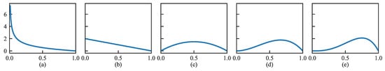
Figure 4. Probability density diagrams of Beta distribution under (a) $\alpha =0.5$, (b) $\alpha =1$, (c) $\alpha =2$, (d) $\alpha =3$, (e) $\alpha =4$.

3.4. SRPL-Based OSFD

Previously, two key ideas—a margin penalty and mixups—were presented separately. This naturally suggests a joint training scheme for SRPL that reduces both empirical risk and open-set risk simultaneously. We therefore define the total SRPL loss L as

$$L=L_{\mathrm{QSAM}-\mathrm{softmax}}+\xi ·L_{\mathrm{IE}},$$

(18)

where $\xi$ is a positive regularization parameter, tuning to balance the model’s ability to distinguish unknown faults from known faults with its ability to correctly classify known faults according to the complexity of the OSFD task in real industrial settings. The overall training procedure of the SRPL-based OSFD model is summarized in Algorithm 2. Below, we discuss additional training techniques from [27] that are incorporated into Algorithm 2 to further improve OSFD performance.

Auxiliary Batch Normalization. According to the total loss in Equation (18), the training dataset ${\mathcal{D}}_{\mathrm{Tr}}$ and the manifold mixups independently are processed separately by the DNN-based classifier f. To avoid confusion arising from differing distributions of known and unknown faults, we incorporate an Auxiliary Batch Normalization (ABN) into f. Two batch-normalization (BN) layers are inserted after the deep embedding function $\Phi$ and before multi-class prediction function $\Psi$. They independently normalize features from ${\mathcal{D}}_{\mathrm{Tr}}$ and from the mixups ${\mathbf{x}}_i^{\mathrm{N}-\mathrm{F}}$. Ablation experiments in Section 4.6 is developed to demonstrate the contribution of ABN.

Focus Training. We develop an alternating training algorithm to efficiently optimize SPRL. In each epoch, Algorithm 2 incorporates a Focus Training (FT) step on $L_{\mathrm{QSAM}-\mathrm{softmax}}$ after the total loss L in Equation (18). The FT step directs the SRPL-based OSFD model to sustain comparable detection performance for unknown faults while simultaneously focusing on classifying known faults. Section 4.6 presents ablation experiments that quantify FT’s contribution.

Algorithm 2: The training procedure of the SRPL-based OSFD model.

In the trained SRPL-based OSFD model, known faults tend to be farther from their reciprocal points than unknown faults. Therefore, for a test sample ${\mathbf{x}}_i^{\mathrm{Te}}$ we use the largest logit $max{l}_{i,k}$, which corresponds to the farthest reciprocal point, as the score for unknown-fault detection. The diagnosis is then given by

$${\widehat{y}}_i=\left\{\begin{array}{cc}{\arg \max }_k{l}_{i,k},\hfill & \mathrm{if}\underset{k}{max}{l}_{i,k}\ge \tau ;\hfill \\ K+1,\hfill & \mathrm{otherwise}.\hfill \end{array}\right.$$

(19)

where $\tau$ denotes the threshold for the unknown-fault detection score, and $K+1$ denotes the class of unknown faults.

4. Experiments and Discussion

4.1. Datasets

The Tennessee–Eastman Process (TEP) [35], a realistic chemical-plant simulation, has become a standard benchmark for evaluating fault-diagnosis methods. In our experiments, we employ the TEP datasets of Russell et al. [36]. The details of datasets are summarized as below.

• Open-set Setting. Following [16], we consider the first 15 faults of the TEP, treating the initial 10 as known faults and the remaining 5 as unknown faults.
• Date Split. For each fault, the abnormal dataset of 480 samples is split so that the first 400 samples form the training dataset ${\mathcal{D}}_{\mathrm{Tr}}$ and the last 80 samples are reserved for validation. A larger abnormal dataset of 800 samples (excluding the first 160 normal samples) serves as the test dataset ${\mathcal{D}}_{\mathrm{Te}}$. We also use a normal dataset of 500 samples as ${\mathcal{D}}_{\mathrm{N}}$ for the NSI-aided manifold mixup.
• Variable Selection. Each sample is represented by 33 variables: 22 continuously measured variables (XMEAS1–22) and 11 manipulated variables (XMV1–11), listed in chronological order. This set excludes time-lagged composition variables (XMEAS23–41) and the constant manipulated variable (XMV12).
• Normalization. Each process variable is normalized into zero mean and unit variance utilizing the mean and standard deviation of ${\mathcal{D}}_{\mathrm{N}}$.

4.2. Evaluation Metrics

We introduce two threshold-independent metrics to evaluate OSFD models—AUROC and OSFDR—as described below.

• We labeled known and unknown fault classes as positive and negative, respectively. While $\tau$ denotes the threshold for the unknown-fault detection score, the receiver operating characteristic (ROC) curve plots the true-positive rate (TPR) against the false-positive rate (FPR). Consequently, the area under the ROC curve (AUROC) measures the model’s ability to distinguish known from unknown faults.
• OSFD rate (OSFDR) adapts open-set classification rate [37] to provide a balanced assessment of a model’s ability to classify known faults and detect unknown faults. Specifically, OSFDR is the area under the curve that plots the correct classification rate (CCR) for known faults versus the false detection rate (FDR) for unknown faults as $\tau$ varies, thereby avoiding bias toward particular dataset compositions. We denote the test datasets that contain only known or only unknown fault samples by ${\mathcal{D}}_{\mathrm{Te}}^{\mathrm{K}}$ and ${\mathcal{D}}_{\mathrm{Te}}^{\mathrm{U}}$, respectively, so that ${\mathcal{D}}_{\mathrm{Te}}={\mathcal{D}}_{\mathrm{Te}}^{\mathrm{U}}\cup {\mathcal{D}}_{\mathrm{Te}}^{\mathrm{U}}$. The CCR and FDR are formulated as

  $$\begin{array}{cc}\hfill \mathrm{CCR}\left(\tau \right)& ={\displaystyle \frac{\left|\right\{\mathbf{x}\mid \mathbf{x}\in {\mathcal{D}}_{\mathrm{Te}}^{\mathrm{K}}\wedge {\arg \max }_k{\mathrm{l}}_k\left(\mathbf{x}\right)=y\wedge {max}_k{\mathrm{l}}_k\left(\mathbf{x}\right)\ge \tau \left\}\right|}{|{\mathcal{D}}_{\mathrm{Te}}^{\mathrm{K}}|}},\hfill \end{array}$$

  (20)

  $$\begin{array}{cc}\hfill \mathrm{FDR}\left(\tau \right)& ={\displaystyle \frac{\left|\right\{\mathbf{x}\mid \mathbf{x}\in {\mathcal{D}}_{\mathrm{Te}}^{\mathrm{U}}\wedge {max}_k{\mathrm{l}}_k\left(\mathbf{x}\right)\ge \tau \left\}\right|}{|{\mathcal{D}}_{\mathrm{Te}}^{\mathrm{U}}|}}.\hfill \end{array}$$

  (21)
  At the smallest $\tau$(i.e., $\tau =0$), CCR equals the closed-set fault diagnosis rate (CSFDR), as

  $$\mathrm{CSFDR}={\displaystyle \frac{\left|\right\{\mathbf{x}\mid \mathbf{x}\in {\mathcal{D}}_{\mathrm{Te}}^{\mathrm{K}}\wedge {\arg \max }_k{\mathrm{l}}_k\left(\mathbf{x}\right)=y\left\}\right|}{|{\mathcal{D}}_{\mathrm{Te}}^{\mathrm{K}}|}}.$$

  (22)

In addition to threshold-independent metrics, we report the F1-score at $\tau$ achieving a given CCR to explicitly illustrated OSFD performance for each fault type. Noted that All reported metrics are averages over five randomized trials.

4.3. Implementation Details

Recently, convolutional neural networks (CNNs) have shown superior representational ability for closed-set fault diagnosis. According to previous research [25,38], one-dimensional CNNs with carefully designed structures are employed for all competing algorithms. The detailed structures are presented in Table 1. To ensure a fair evaluation of OSFD performance, it is essential that the same structures are utilized as the embedding function $\Phi$, with the decoder and generator serving as the transposed versions of $\Phi$. Notably, the inputs suitable for these one-dimensional CNNs consist of samples sized $3\times 33$, which are derived from the general dynamic data expansion scheme with a lagged length of 2 detailed in [38].

Table 1. The Structures of CNNs.

Algorithm	Deep Embedding Function $\mathbf{\Phi }$	Multi-Class Prediction Function $\mathbf{\Psi }$	Decoder or Generator	Discriminator
Softmax OpenMax GCPL RPL SRPL	Conv(3, 64) 1/tanh Conv(64, 256)/tanh Conv(256, 512)/tanh Conv(512, 99)	Linear(99, 128) 2/tanh Linear(128, 128)/tanh Linear(128, 1)/sigmoid	✗	✗
MLOSR CROSR			DConv(99, 128) 3/tanh DConv(128, 64)/tanh DConv(64, 32)/tanh DConv(32, 3)
ARPL				Conv(3, 64)/tanh Conv(64, 256)/tanh Conv(256, 512)/tanh Conv(512, 1)/sigmoid

¹ Conv($·,·$) denote convolution layer with its number of input and output filters. ² Linear($·,·$) denote fully connected layer with its number of input and output nodes. ³ DConv($·,·$) denote transposed convolution layer with its number of input and output filters.

The FT step, which relies solely on $L_{\mathrm{QSAM}-\mathrm{softmax}}$, is incorporated after the total loss L in each training epoch. Another advantage of this integration is that it renders SRPL less sensitive to the regularization parameter $\xi$ between $L_{\mathrm{QSAM}-\mathrm{softmax}}$ and $L_{\mathrm{IE}}$. Consequently, it yields satisfactory outcomes in preserving classification performance for known faults while maintaining comparable detection performance for unknown faults when $\xi$ is set to 1. In the absence of prior information regarding the complexity of the OSFD task in an industrial setting, it is reasonable to treat these two losses as equal, and we do not make further adjustments. Additionally, the value $m=0.5$ is selected based on validation data, as it produces the best performance in closed-set fault diagnosis according to the CSFDR metric. Furthermore, all models are trained using the Adam optimizer with a learning rate of 0.001, a batch size of 64, and a maximum of 50 epochs.

4.4. Experimental Results

We evaluated our proposed OSFD method SRPL against state-of-the-art algorithms, including discriminative models—threshold-based Softmax, OpenMax [21], general convolutional prototype learning (GCPL) [22], RPL [26], and adversarial RPL (ARPL) [27]; generative models—multitask OSR (MLOSR) [23] and classification-reconstruction OSR (CROSR) [24]. The experimental results, presented as ROC and OSFDR curves, appear in Figure 5 and Figure 6, and the corresponding metrics AUROC and OSFDR are reported in Table 2. The rightmost column of Table 2 displays the CSFDR, which evaluates the performance of closed-set fault diagnosis using OSFD models, specifically focusing on the CCR at the smallest threshold ($\tau =0$). The average CSFDR is approximately 80%, suggesting that when $\tau$ achieves a 75% CCR, the classification ability for known faults is only slightly affected to accommodate the detection of unknown faults. Consequently, the F1-scores at $\tau$ corresponding to a 75% CCR, which are just below 80% (referred to as F1-scores@CCR = 75%), are used to clearly demonstrate the OSFD performance for each known faults and all unknown faults treated as a single class. For SRPL(w/o MM), SRPL, and some competing algorithms such GCPL and RPL, we provide F1-scores@CCR=75% in Table 3. The embedding feature visualizations for these methods are also presented in Figure 7. Noted that, SRPL(w/o MM) refers to SRPL without the incorporation of NSI-based Manifold Mmixup (MM).

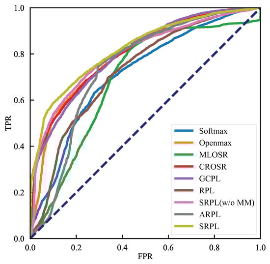
Figure 5. The experimetal results in terms of ROC curves.

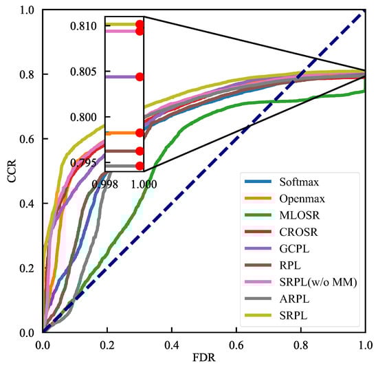
Figure 6. The experimetal results in terms of OSFDR curves.

Table 2. The experimetal results in terms of AUROCs, OSFDRs and CSFDRs (mean ± std%).

Method	AUROC	OSFDR	CSFDR
Softmax	71.36 (±0.57)	62.51 (±5.77)	79.82 (±0.96)
OpenMax [21]	79.70 (±1.29)	67.89 (±5.44)	79.82 (±0.96)
MLOSR [23]	68.84 (±1.01)	52.73 (±2.81)	78.97 (±1.47)
CROSR [24]	80.21 (±1.78)	67.73 (±0.77)	78.97 (±2.26)
GCPL [22]	80.35 (±0.77)	67.73 (±2.07)	80.44 (±0.73)
RPL [26]	72.56 (±1.10)	62.43 (±1.58)	79.62 (±2.52)
SRPL(w/o MM)	80.01 (±2.23)	68.63 (±3.72)	80.94 (±0.99)
ARPL [27]	74.07 (±3.48)	61.43 (±2.92)	79.46 (±6.94)
SRPL	82.32 (±0.14)	71.50 (±1.67)	81.02 (±1.28)

Table 3. The experimetal results in terms of F1-scores@CCR = 75% (mean ± std%).

Method	GCPL	RPL	SRPL(w/o MM)	SRPL
1	99.37 (±0.13)	99.56 (±0.08)	98.34 (±0.77)	99.56 (±0.15)
2	98.67 (±0.20)	98.86 (±0.22)	98.34 (±0.37)	98.55 (±0.18)
3	41.41 (±6.90)	36.87 (±2.92)	34.19 (±6.94)	36.39 (±6.48)
4	84.96 (±0.07)	69.66 (±0.18)	79.13 (±0.20)	84.58 (±0.14)
5	71.24 (±3.01)	70.45 (±2.89)	70.36 (±1.76)	78.19 (±0.71)
6	99.50 (±0.36)	99.43 (±0.88)	99.24 (±0.66)	99.37 (±0.16)
7	99.87 (±0.04)	100.00 (±0.00)	99.94 (±0.57)	100.00 (±0.00)
8	49.67 (±0.27)	51.52 (±0.87)	49.80 (±1.96)	49.37 (±1.45)
9	20.11 (±2.34)	29.27 (±4.47)	36.52 (±2.39)	29.25 (±2.30)
10	43.40 (±5.22)	40.29 (±2.81)	46.41 (±5.38)	52.79 (±5.29)
unknown	55.50 (±2.13)	47.94 (±1.93)	52.55 (±1.97)	59.54 (±1.63)
macro avg	69.43 (±1.88)	67.62 (±1.57)	69.53 (±2.09)	71.60 (±1.68)

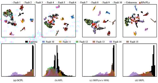
Figure 7. The experimetal results in terms of the embedding feature visualizations. (1) The first row presents a visualization of embedding features, where 2D features are projected using t-SNE [39]. Dots of varying colors represent different fault types; specifically, the colorful dots correspond to known faults, while the black dots indicate unknown faults. Red triangles signify reciprocal points or prototypes. (2) The second row illustrates the distribution of maximum logits, which serve as detection scores. The histogram employs different colors to represent various fault types; in this case, the black bars correspond to known faults, while the colorful bars represent unknown faults.

4.5. Performance Comparison

ROC Curve and AUROC. Figure 5 and Table 2 compare ROC curves and AUROCs. Some competitive algorithms, such as CROSR and GCPL, improved distinguishability between known and unknown faults through different schemes, yielding an AUROC of about 80%. Our SRPL(w/o MM), trained only on known faults, achieved a comparable AUROC of 80.01%. Adding NSI-aided manifold mixup further improved performance: SRPL reached an AUROC of 82.32%. It is observed in Figure 7d that the global open space represented by reciprocal points is contracted surrounded by known faults. These results indicate that SRPL(w/o MM) and SRPL better identify unknown faults by indirectly and directly estimating the unknown-fault distribution.

OSFDR curve and OSFDR. Figure 6 and Table 2 compare OSFDR curves and OSFDRs, which are more comprehensive metrics for evaluating OSFD performance. Most competing algorithms yielded relatively low OSFDRs despite achieving comparable AUROCs. This pattern indicates they traded off some ability to classify known faults in order to improve identification of unknown faults. By contrast, SRPL(w/o MM) already outperformed other methods, achieving an OSFDR of 68.63%, and SRPL increased the OSFDR further to 71.50%. Together, these results indicate that SRPL preserves classification performance on known faults while maintaining comparable detection performance for unknown faults. This improvement may stem from the QSAM-based softmax loss. Figure 7d illustrates that SRPL yields more discriminative features that enhance diagnosability of known faults, and it reduces over-allocated embedding space, thereby reserving more capacity to distinguish unknown from known faults.

F1-scores@CCR = 75%. Table 3 reports F1-scores at CCR = 75%, which further underscore SRPL’s ability to improve detection of unknown faults and classification of known faults simultaneously. When CCR is 75% for all methods, SRPL attains the highest F1-scores for unknown faults, with SRPL(w/o MM) ranking second order. The results align with those of AUROC metric and again indicates that NSI-aided manifold mixup benefits identify unknown faults. Moreover, SRPL(w/o MM) also performs well on known-fault F1-scores when it leads on unknown-fault F1-score, consistent with the results of OSFDR metric. After introducing NSI-aided manifold mixup, SRPL particularly yields higher F1-scores across all known faults, with particularly marked gains for faults 5 and 10. After incorporating NSI-aided manifold mixup, SRPL produces higher F1-scores for all known faults, with particularly large improvements for faults 5 and 10. As discussed above for NSI-aided manifold mixup, the learnable embedding function $\Phi$ pushes the decision boundary for unknown faults (${\mathcal{O}}_{\mathrm{G}}$ represented by reciprocal points) away from known faults. Note that ${\mathcal{O}}_{\mathrm{N}}\subset {\mathcal{O}}_{\mathrm{G}}$, and these incipient faults differ from the normal state (${\mathcal{O}}_{\mathrm{N}}$) by only small-amplitude deviations. As shown in Figure 7d, faults 5 and 10 lie farther from the reciprocal points on the hypersphere manifold, which accounts for their relatively higher F1-scores.

Overall, these results demonstrate that SRPL(w/o MM) more effectively identifies unknown faults while preserving classification accuracy for known faults, and that NSI-aided manifold mixups further enhance SRPL’s reliability. Unlike post-processing OSR algorithms, these gains largely stem from estimating the unknown fault distribution during training. Below, we provide a detailed analysis of the state-of-the-art OSR algorithms introduced in OSFD.

• Discriminative Model. OpenMax extends closed-set oriented Softmax to an open-set model, raising AUROC compared with threshold-based Softmax. However, because OpenMax was designed to trade off known-fault classification against unknown-fault detection, it sacrificed some known-fault classification performance for OSFD tasks and attained a relatively low OSFDR of 67.89%. GCPL addressed the tendency for over-allocated embedding space by adding a center loss to increase intra-class compactness for each known fault, as shown in Figure 7a. Although GCPL achieves a higher AUROC than OpenMax, 80.35% versus 79.70%, it still yields a low OSFDR of 67.73%.
• Generative Model. MLOSR performs poorly on OSFD, achieving only 68.84% AUROC and 52.73% OSFDR, despite the widespread use of reconstruction error as a detection score in fault detection task. This outcome suggests that unknown faults can be reconstructed as effectively as known faults when the two types share strong similarities, which makes reconstruction-error–based schemes ill-suited for the OSFD task. Although CROSR adapts OpenMax by refining embedding features with a decoder, it still attains a similarly low OSFDR value as OpenMax.
• RPL Model. RPL models the unknown-class distribution by separating known classes with reciprocal points, which yields robust discrimination between known and unknown images [27]. However, when applied to the OSFD task, RPL and ARPL performs worse than the thresholded Softmax, with OSFDR ranging from 62.43% to 62.51%. This outcome supports our argument in Section 1: similarities among different faults conflict with the reciprocal-point assumption for diagnosing known faults, and the resulting over-allocated embedding space further degrades unknown-fault detection. Figure 7b visualizes this deterioration in the embedding space. Moreover, ARPL likewise generates confusing samples via a GAN as unknown classes. While the confusing sample raises the AUROC for unknown fault detection from 72.56% to 74.7%, OSFDR falls from 62.43% to 61.43% compared to RPL. This decline of OSFDR suggests that image-oriented synthesized samples without careful designing for industrial settings may impair learning of discriminative features for known faults, particularly when known and unknown faults exhibit strong similarity. By contrast, SRPL(w/o MM) introducing RPL into the hyperspherical manifold substantially improves the AUROC and OSFDR, and SRPL and achieves even greater gains.

4.6. Ablation Study

We first analyze the contributions of two key ideas—a margin penalty and mixups—via ablation experiments.

QSAM-based Softmax Loss. The rightmost column of Table 2 displays CSFDRs for evaluating the performance of closed-set fault diagnosis using OSFD models. Without considering SRPL, GCPL and SRPL(w/o MM) achieve the highest CSFDRs, 80.44% and 80.94% respectively, because they actively optimize embedding features to be more discriminative using center loss and the QSAM-based softmax loss. The red dots in Figure 6, which mark the intersections of the OSFDR curves with the $\mathrm{FDR}=1$ line, correspond to the CSFDRs and further indicate that that more discriminative features help prevent overfitting in the OSFD task. In addition, embedding visualizations in Figure 7a–c show that SRPL(w/o MM) produces more compact clusters and larger separations between known faults than GCPL and RPL. The above all prove the advantage that the QSAM-based softmax loss reduces empirical classification risk on the hypersphere manifold. Compared with RPL, SRPL(w/o MM) based the QSAM-based softmax loss preserves classification performance on known faults while reducing over-allocated embedding space, which improves detection of unknown faults.

NSI-aided Manifold Mixup. Table 2 and Table 3 show that NSI-aided manifold mixup substantially improves SRPL(w/o MM) on AUROC, OSFDR, and F1-score metrics. In particular, NSI-aided manifold mixup markedly enhances detection of unknown faults: the F1-score of SRPL increases by 6.99% relative to the one of SRPL(w/o MM). Comparing Figure 7c,d, the global open space represented by reciprocal points is substantially reduced, and the distributions of maximum logits for known and unknown faults become more separable. These findings indicate that NSI-aided manifold mixup reduces open-set risk arising from the global open space. Consequently, fewer known faults are misidentified as unknown, and the resulting discriminative embedding features better support correct classification.

Apart from the above merits of the NSI-aided manifold mixup bringing for SRPL, we further analyze the contribution of each part of the NSI-aided manifold mixup through ablation experiments as follows.

Mixups with Various $\alpha$ based on ABN and FT. We conducted an analysis using various $\alpha$ values based on ABN and FT that are the training tricks for NSI-aided manifold mixup. Utilizing different $\alpha$ values from the Beta($\alpha$, $\alpha$) distribution for sampling ${\gamma }_2$, we evaluated the OSFD performance of SRPL, which employs NSI-aided manifold mixup, along with SRPL trained without ABN, denoted as SRPL(w/o ABN), and SRPL trained without FT, denoted as SRPL(w/o FT). The results are illustrated in Figure 8a,b. Consistent with our intuition discussed in Section 3.3, SRPL demonstrated optimal performance at $\alpha =2$. It is advantageous for $\alpha =2$ to synthesize unknown faults that fall within the global open space ${\mathcal{O}}_{\mathrm{G}}$ while less hinder the reduction of ${\mathcal{O}}_{\mathrm{G}}$, which can be observed in Figure 7d. Furthermore, the OSFD performance declined in the absence of either ABN or FT across all $\alpha$ values, attributable to the deviation introduced by NSI-aided manifold mixup. When FT was incorporated into SRPL(w/o FT) to enhance the classification of known faults, the performance of SRPL improved progressively, particularly for OSFDR. Conversely, the performance of SRPL(w/o ABN) was inferior to that of SRP, aligning with our hypothesis that the mixed distribution of known faults and mixups adversely impacts OSFD performance. Thus, the integration of ABN and FT schemes can further enhance SRPL, resulting in superior performance compared to the alternatives.

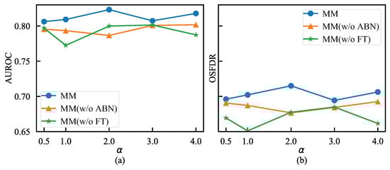
Figure 8. The ablation experimental results of the NSI-aided manifold mixup with or without ABN and FT under different $\alpha$. (a) The ablation experimetal results in terms of AUROCs. (b) The ablation experimetal results in terms of OSFDRs.

Mixups with Manifold and Normal State Information. We conducted an additional analysis of NSI-aided manifold mixup, examining scenarios with and without manifold assistance and with or without normal state information. We assessed the OSFD performance of SRPL, which incorporated NSI-aided Manifold Mixup (MM), Input Mixup (IM), the direct use of normal samples as unknown faults denoted as MM(w/o fault), and manifold mixup without the aid of Normal State Information denoted MM(w/o NSI). The results are presented in Figure 9. Compared to IM, MM demonstrated improved OSFD performance, as manifold mixups can be optimized to more effectively represent unknown-fault patterns, as detailed in Section 3.3. Furthermore, the primary distinctions between MM, MM(w/o fault), and MM(w/o NSI) lie in the incorporation of auxiliary information from known faults and normal samples, which enhances the reliability of virtual unknown samples. Overall, the results indicate that a manifold combination of known faults and normal samples can significantly enhance OSFD performance.

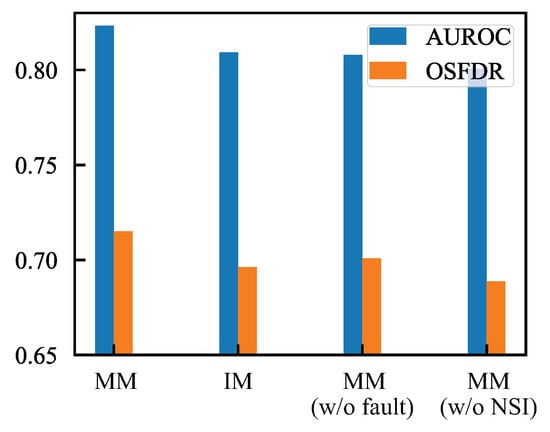
Figure 9. The ablation experimental results of the NSI-aided manifold mixup with or without manifold and NSI.

5. Conclusions

When faced with a new fault of an unknown type in realistic industrial processes, conventional closed-set fault diagnosis models often misclassify it as one of the known fault types. This paper formulates an open-set fault diagnosis task designed to differentiate unknown faults from known faults while accurately classifying the latter. However, the application of state-of-the-art reciprocal point learning to this open-set fault diagnosis task presents two significant challenges in industrial contexts: how to minimize the empirical classification risk for known faults and how to address the open space risk associated with potentially unknown faults. To tackle these challenges, we propose a hypersphere-guided reciprocal point learning approach. First, we introduce a softmax loss function that incorporates an angular penalty within a unit hypersphere, enhancing the discrimination of known faults. Additionally, we develop a manifold mixup technique, supported by normal-state information, to effectively estimate the distribution of unknown faults in a straightforward manner. Comprehensive experiments conducted from various perspectives demonstrate the superiority of our proposed method compared to existing state-of-the-art open-set recognition algorithms. Future research directions include extending the proposed model to diagnose unknown faults in time-series data and further investigating the identified unknown faults.

References

- Melo, A.; Câmara, M.M.; Pinto, J.C. Data-Driven Process Monitoring and Fault Diagnosis: A Comprehensive Survey. Processes 2024, 12, 251. [Google Scholar] [CrossRef]
- Yan, W.; Wang, J.; Lu, S.; Zhou, M.; Peng, X. A Review of Real-Time Fault Diagnosis Methods for Industrial Smart Manufacturing. Processes 2023, 11, 369. [Google Scholar] [CrossRef]
- Chae, S.G.; Yun, G.H.; Park, J.C.; Jang, H.S. Adaptive Structured Latent Space Learning via Component-Aware Triplet Convolutional Autoencoder for Fault Diagnosis in Ship Oil Purifiers. Processes 2025, 13, 3012. [Google Scholar] [CrossRef]
- He, S.; Zhou, F.; Tan, X.; Hu, G.; Ruan, J.; He, S. Research on Mechanical Fault Diagnosis Method of Isolation Switch Based on Variational Autoencoder. Processes 2025, 13, 2388. [Google Scholar] [CrossRef]
- Wang, W.; Xu, J.; Li, X.; Tong, K.; Shi, K.; Mao, X.; Wang, J.; Zhang, Y.; Liao, Y. ResNet + Self-Attention-Based Acoustic Fingerprint Fault Diagnosis Algorithm for Hydroelectric Turbine Generators. Processes 2025, 13, 2577. [Google Scholar] [CrossRef]
- Wen, L.; Li, X.; Gao, L.; Zhang, Y. A New Convolutional Neural Network-Based Data-Driven Fault Diagnosis Method. IEEE Trans. Ind. Electron. 2018, 65, 5990–5998. [Google Scholar] [CrossRef]
- Li, S.; Gong, Z.; Wang, S.; Meng, W.; Jiang, W. Fault Diagnosis Method for Rolling Bearings Based on a Digital Twin and WSET-CNN Feature Extraction with IPOA-LSSVM. Processes 2025, 13, 2779. [Google Scholar] [CrossRef]
- Jiang, X.; Ge, Z. Data Augmentation Classifier for Imbalanced Fault Classification. IEEE Trans. Autom. Sci. Eng. 2021, 18, 1206–1217. [Google Scholar] [CrossRef]
- Zhuo, Y.; Ge, Z. Gaussian Discriminative Analysis Aided GAN for Imbalanced Big Data Augmentation and Fault Classification. J. Process Control 2020, 92, 271–287. [Google Scholar] [CrossRef]
- Wu, S.; Yang, L.; Tao, L. Synergistic WSET-CNN and Confidence-Driven Pseudo-Labeling for Few-Shot Aero-Engine Bearing Fault Diagnosis. Processes 2025, 13, 1970. [Google Scholar] [CrossRef]
- Li, S.; Liu, Z.; Yan, Y.; Han, K.; Han, Y.; Miao, X.; Cheng, Z.; Ma, S. Research on a Small-Sample Fault Diagnosis Method for UAV Engines Based on an MSSST and ACS-BPNN Optimized Deep Convolutional Network. Processes 2024, 12, 367. [Google Scholar] [CrossRef]
- Ko, T.; Kim, H. Fault Classification in High-Dimensional Complex Processes Using Semi-Supervised Deep Convolutional Generative Models. IEEE Trans. Ind. Inform. 2020, 16, 2868–2877. [Google Scholar] [CrossRef]
- Li, S.; Luo, J.; Hu, Y. Semi-Supervised Process Fault Classification Based on Convolutional Ladder Network with Local and Global Feature Fusion. Comput. Chem. Eng. 2020, 140, 106843. [Google Scholar] [CrossRef]
- Hu, Z.; Jiang, P. An Imbalance Modified Deep Neural Network with Dynamical Incremental Learning for Chemical Fault Diagnosis. IEEE Trans. Ind. Electron. 2018, 66, 540–550. [Google Scholar] [CrossRef]
- Rodríguez-Ramos, A.; Rivera Torres, P.J.; Silva Neto, A.J.; Llanes-Santiago, O. Machine Learning-Based Condition Monitoring with Novel Event Detection and Incremental Learning for Industrial Faults and Cyberattacks. Processes 2025, 13, 2984. [Google Scholar] [CrossRef]
- Yu, W.; Zhao, C. Broad Convolutional Neural Network Based Industrial Process Fault Diagnosis with Incremental Learning Capability. IEEE Trans. Ind. Electron. 2020, 67, 5081–5091. [Google Scholar] [CrossRef]
- Wang, C.; Xin, C.; Xu, Z. A Novel Deep Metric Learning Model for Imbalanced Fault Diagnosis and toward Open-Set Classification. Knowl.-Based Syst. 2021, 220, 106925. [Google Scholar] [CrossRef]
- Zhuo, Y.; Ge, Z. Auxiliary Information-Guided Industrial Data Augmentation for Any-Shot Fault Learning and Diagnosis. IEEE Trans. Ind. Inform. 2021, 17, 7535–7545. [Google Scholar] [CrossRef]
- Yang, J.; Zhou, K.; Li, Y.; Liu, Z. Generalized Out-of-Distribution Detection: A Survey. Int. J. Comput. Vis. 2024, 132, 5635–5662. [Google Scholar] [CrossRef]
- Geng, C.; Huang, S.J.; Chen, S. Recent Advances in Open Set Recognition: A Survey. IEEE Trans. Pattern Anal. Mach. Intell. 2020, 43, 3614–3631. [Google Scholar] [CrossRef]
- Bendale, A.; Boult, T.E. Towards Open Set Deep Networks. In Proceedings of the IEEE Conference on Computer Vision and Pattern Recognition, Las Vegas, NV, USA, 27–30 June 2016; pp. 1563–1572. [Google Scholar] [CrossRef]
- Yang, H.M.; Zhang, X.Y.; Yin, F.; Yang, Q.; Liu, C.L. Convolutional Prototype Network for Open Set Recognition. IEEE Trans. Pattern Anal. Mach. Intell. 2022, 44, 2358–2370. [Google Scholar] [CrossRef]
- Oza, P.; Patel, V.M. Deep CNN-Based Multi-Task Learning for Open-Set Recognition. arXiv 2019, arXiv:1903.03161. [Google Scholar]
- Yoshihashi, R.; Shao, W.; Kawakami, R.; You, S.; Iida, M.; Naemura, T. Classification-Reconstruction Learning for Open-Set Recognition. In Proceedings of the IEEE Conference on Computer Vision and Pattern Recognition, Long Beach, CA, USA, 15–20 June 2019; pp. 4011–4020. [Google Scholar] [CrossRef]
- Perera, P.; Morariu, V.I.; Jain, R.; Manjunatha, V.; Wigington, C.; Ordonez, V.; Patel, V.M. Generative-Discriminative Feature Representations for Open-Set Recognition. In Proceedings of the IEEE Conference on Computer Vision and Pattern Recognition, Piscataway, NJ, USA, 21–26 July 2020; pp. 11811–11820. [Google Scholar] [CrossRef]
- Chen, G.; Qiao, L.; Shi, Y.; Peng, P.; Li, J.; Huang, T.; Pu, S.; Tian, Y. Learning Open Set Network with Discriminative Reciprocal Points. In Proceedings of the European Conference on Computer Vision, Glasgow, UK, 23–28 August 2020; pp. 507–522. [Google Scholar] [CrossRef]
- Chen, G.; Peng, P.; Wang, X.; Tian, Y. Adversarial Reciprocal Points Learning for Open Set Recognition. IEEE Trans. Pattern Anal. Mach. Intell. 2021, 44, 8065–8081. [Google Scholar] [CrossRef] [PubMed]
- Liu, W.; Wen, Y.; Yu, Z.; Yang, M. Large-Margin Softmax Loss for Convolutional Neural Networks. In Proceedings of the International Conference on Machine Learning, New York, NY, USA, 19–24 June 2016; pp. 507–516. [Google Scholar]
- Deng, J.; Guo, J.; Xue, N.; Zafeiriou, S. ArcFace: Additive Angular Margin Loss for Deep Face Recognition. In Proceedings of the IEEE Conference on Computer Vision and Pattern Recognition, Long Beach, CA, USA, 16–20 June 2019; pp. 4685–4694. [Google Scholar] [CrossRef]
- Zhao, H.; Shi, Y.; Tong, X.; Ying, X.; Zha, H. Qamface: Quadratic Additive Angular Margin Loss for Face Recognition. In Proceedings of the International Conference on Image Processing, Abu Dhabi, United Arab Emirates, 25–28 October 2020; pp. 1901–1905. [Google Scholar] [CrossRef]
- Scheirer, W.J.; De Rezende Rocha, A.; Sapkota, A.; Boult, T.E. Toward Open Set Recognition. IEEE Trans. Pattern Anal. Mach. Intell. 2013, 35, 1757–1772. [Google Scholar] [CrossRef]
- Verma, V.; Lamb, A.; Beckham, C.; Najafi, A.; Mitliagkas, I.; Lopez-Paz, D.; Bengio, Y. Manifold Mixup: Better Representations by Interpolating Hidden States. In Proceedings of the International Conference on Machine Learning, Los Angeles, CA, USA, 9–15 June 2019; pp. 6438–6447. [Google Scholar]
- Zhou, D.W.; Ye, H.J.; Zhan, D.C. Learning Placeholders for Open-Set Recognition. In Proceedings of the IEEE Conference on Computer Vision and Pattern Recognition, Piscataway, NJ, USA, 19–25 June 2021; pp. 4399–4408. [Google Scholar] [CrossRef]
- Tokozume, Y.; Ushiku, Y.; Harada, T. Between-Class Learning for Image Classification. In Proceedings of the IEEE Conference on Computer Vision and Pattern Recognition, Salt Lake City, UT, USA, 18–23 June 2018; pp. 5486–5494. [Google Scholar] [CrossRef]
- Downs, J.; Vogel, E. A Plant-Wide Industrial Process Control Problem. Comput. Chem. Eng. 1993, 17, 245–255. [Google Scholar] [CrossRef]
- Russell, E.L.; Chiang, L.H.; Braatz, R.D. Fault Detection in Industrial Processes Using Canonical Variate Analysis and Dynamic Principal Component Analysis. Chemom. Intell. Lab. Syst. 2000, 51, 81–93. [Google Scholar] [CrossRef]
- Dhamija, A.R.; Günther, M.; Boult, T.E. Reducing Network Agnostophobia. In Proceedings of the Advances in Neural Information Processing Systems, Montréal, QC, Canada, 3–8 December 2018; pp. 9157–9168. [Google Scholar]
- Li, S.; Luo, J.; Hu, Y. Towards Interpretable Process Monitoring: Slow Feature Analysis Aided Autoencoder for Spatiotemporal Process Feature Learning. IEEE Trans. Instrum. Meas. 2021, 71, 1–11. [Google Scholar] [CrossRef]
- Maaten, L.V.D.; Hinton, G. Visualizing Data Using T-SNE. J. Mach. Learn. Res. 2008, 9, 2579–2605. [Google Scholar]
Disclaimer/Publisher’s Note: The statements, opinions and data contained in all publications are solely those of the individual author(s) and contributor(s) and not of MDPI and/or the editor(s). MDPI and/or the editor(s) disclaim responsibility for any injury to people or property resulting from any ideas, methods, instructions or products referred to in the content. |
© 2025 by the authors. Licensee MDPI, Basel, Switzerland. This article is an open access article distributed under the terms and conditions of the Creative Commons Attribution (CC BY) license (https://creativecommons.org/licenses/by/4.0/).