Abstract
Modular process plants represent a promising strategy to address the increasing need for flexibility and accelerated market deployment in the production of fine and specialty chemicals. However, these modular systems are inherently susceptible to wear and fault development, while condition monitoring methods tailored to such systems remain scarce. This study presents a proof of concept for a targeted fault diagnosis approach of the modular hydraulic systems of such modular process plants and reports on its experimental validation. The methodology comprises two stages: First, model-based symptoms are calculated independently for each module and subsequently utilized within a centralized diagnostic system. This rule-based diagnosis incorporates generalized module interactions, quantified fault degrees, and the plant topology. Importantly, uncertainties arising from measurement equipment, model fidelity, and parameter variability are incorporated and systematically propagated throughout the diagnosis. The validation was conducted on a modular test rig specifically designed to simulate a range of single-fault scenarios across more than 1200 stationary operating points. The results underscore the robustness of the proposed approach: the correct fault was consistently identified, with the estimated fault magnitudes closely aligning with the actual values, exhibiting an average discrepancy of 0.029 for internal leakage of a positive displacement pump. The overall discrepancy for the experimental validation of all fault types was 0.12. Notably, no false alarms were observed, and the displayed uncertainty was considered plausible, though there remains potential for refinement. In summary, this study demonstrates the successful application of model-based symptoms for a rule-based diagnosis, representing a significant advancement toward reliable fault detection in modular hydraulic systems.
1. Introduction
Global market pressure and the trend toward increased product individualization are driving the need for greater flexibility and shorter time-to-market in fine and specialty chemicals production [1]. One solution gaining momentum is the conversion from conventional batch production to modular continuous production [2]. Modular production is based on modular process plants that consist of modular process equipment for each process step. These modules are linked together to form a bespoke plant configuration tailored to the production of a specific product [3]. After production, the plant can be disassembled and reconfigured for the next product recipe, while the modules themselves remain unaltered.
These modules are engineered to operate over a broad range rather than being optimized for a single operating point. This versatility supports their integration into various modular setups, enhancing their adaptability to different production configurations. However, this also means that modules frequently operate under partial load, which can contribute to accelerated wear on components [4]. The safe and reliable operation of process plants relies on the detection of changes (fault detection), finding its cause (fault isolation) and the quantification of its effect (fault identification). Together, this is called fault diagnosis. Consequently, a robust fault diagnosis system is essential to continuously monitor module performance, ensuring that operational integrity is maintained and that modules consistently deliver their intended function.
The task of fault diagnosis for modular process plants presents several inherent challenges. Due to the frequent reconfiguration of these plants to accommodate different product requirements, their topology is subject to regular changes, while the modules themselves remain unaltered once manufactured. The knowledge about the module behavior lies with their manufacturers, while the plant operators are the only ones who know about the plant topology. The setup of a flexible fault diagnosis system for modular plants has to be accomplished in a timely manner with appropriate effort. This limits the available options for fault diagnosis solutions.
Purely model-based approaches rely on the comprehensive knowledge of the plant’s overall behavior [5]. The description of the whole plant is time consuming, especially since this step must be repeated for every adaptation of the modular plant. Data-driven approaches require large amounts of historical data for training purposes. The successful application of these methods typically requires labeled datasets containing operational data under normal conditions and associated maintenance records [6]. For the flexible modular process plant, this is a nearly impossible challenge, as the individual plant compositions are highly specific and only operate for a limited time. Consequently, data on its operation are scarce. Expert knowledge-based approaches leverage the knowledge and experience of operators and maintenance personnel to identify patterns or symptoms indicative of specific faults [7]. This expertise can be formalized within artificial intelligence frameworks known as expert systems. However, these approaches depend heavily on the availability of specialized knowledge, which may be lacking for the novel configurations inherent to modular process plants. Subsequently, such methods may not be directly applicable to the flexible and adaptive nature of modular production systems, where expert familiarity with each unique configuration is not guaranteed.
To the best of the authors’ knowledge, there are no suitable fault diagnosis solutions available that take the requirements of a modular process plant into account. These requirements include high adaptability to varying plant configurations, the integration of distributed knowledge pertaining to the behavior of individual modules and the overall plant topology, as well as the utilization of existing measurement infrastructure. In light of the absence of a comprehensive solution for this challenge, the authors previously proposed a hybrid fault diagnosis framework tailored for modular process plants, as detailed in [8]. It unfolds in two steps. First, model-based symptoms are calculated independently for every module. Second, these module-level symptoms are input into a central diagnostic system that leverages knowledge of the specific module interactions, considering the current plant topology. By combining a model-based approach at the module level with a knowledge-based diagnostic framework at the plant level, this method effectively addresses the challenges of condition monitoring in modular process plants.
The prior publication primarily focused on the conceptual design of the overall condition monitoring framework with particular emphasis on the first stage, i.e., the generation of model-based symptoms at the module level. The present work shifts attention to the second stage: the centralized diagnostic system, which applies rules of generalized module interaction to evaluate the symptoms and perform fault isolation and identification. Most modular process plants rely on modules for fluid handling, dosing and mixing in early process stages. Therefore, this study will present a diagnostic system for such modular hydraulic systems. The examined scenarios are constrained to the occurrence of a single fault at a time. Extensions of the methodology to support the diagnosis of multiple concurrent faults are the subject of ongoing research and will be addressed in future publications.
The structure of this paper is as follows: Section 2 provides an overview of model-based condition monitoring approaches to situate the proposed methodology within the broader research landscape. Section 3 describes the implementation of the model-based symptom generation and the rule-based diagnostic framework, employing a generalized and simplified modular plant setup. Section 4 presents the experimental validation of the approach, detailing the test rig, examined fault scenarios, and diagnostic performance. A discussion of the results is provided in Section 5, which is followed by concluding remarks and directions for future work in Section 6.
2. Model-Based Condition Monitoring
Model-based approaches to fault detection and diagnosis rely on a physical model of the process to be observed, which describes its behavior with high fidelity. A parallel simulation of the process within the model calculates the expected state and output variables under given input conditions. This creates an analytical redundancy [9]. Deviations between the model-generated outputs and the actual measured process values, referred to as residuals, serve as indicators of discrepancies in process behavior, potentially signaling the presence of faults [10].
The methods of model-based condition monitoring and fault diagnosis differ mainly in the evaluation of the analytical redundancy. Prominent methods in this domain include parameter identification, parity equations, and state observers [11].
2.1. Parameter Identification
Process models establish relationships between input and output variables. The internal process parameters are usually not measurable but must be inferred through estimation. Parameter identification techniques continuously estimate these parameters during system operation, and deviations in their values over time may indicate system changes or developing faults [12,13]. For processes exhibiting linear behavior, the model is typically formulated as a system of linear equations. The difference between the model’s output and the actual system output is minimized using optimization techniques, such as the least squares method. This involves an iterative adjustment of model parameters at each computational step to minimize the residual error [14].
Alternative optimization strategies, such as the downhill simplex algorithm, offer improved estimation accuracy but at the expense of increased computational effort [11]. More advanced recursive techniques, including recursive least squares (RLS) and extended least squares (ELS), have been developed to improve numerical efficiency and adaptability. These methods restructure the estimation problem to enhance real-time applicability and robustness [15].
2.2. Parity Equations
The differences between the calculated model outputs and the actual signals obtained from the physical process are referred to as residuals. The residuals therefore quantify the discrepancy between the process and the model. The residuals can be formulated using transfer functions or via state-space formulations.
For fault-free behavior of the process and an ideal model without noise, the output variables of the model align exactly with the process. This means that the residuals are zero. In reality, however, there is always a model uncertainty, as the model is only an approximation of reality. The output variables of the real process are also distorted by noise. If the process is superimposed by additive faults, these have a direct effect on the output fault. Faults in the input variables are filtered by the process model [16].
For the reliable detection of faults using the parity equations, meaningful threshold values must be defined for the residuals. These thresholds must be carefully selected based on the known model uncertainties and the statistical properties of the process noise. Analyzing the magnitude, direction, and temporal pattern of the residuals enables not only fault detection (i.e., the recognition of abnormal behavior) but also supports fault isolation (identification of the fault’s location or type) and fault identification (quantification of fault magnitude) [17].
2.3. State Observers
State observers also utilize the output error between a measured and calculated process output. These observers estimate the internal (often unmeasurable) state variables of a system using available input and output measurements. The estimated state variables are subsequently used to reconstruct the process output through the system model.
If the process and model match, the output error disappears. If the process is influenced by disturbances or additive faults, an error remains in the calculated state variables and thus also an output error depending on the disturbances. This error serves as a primary residual signal for detecting anomalies in the system. For fault isolation, fault-specific residuals—analogous to those used in parity-based methods—must be derived to distinguish between different fault types [18].
A significant advancement in the domain of state observers is the Kalman filter, which was originally introduced by Rudolf Kalman in 1960 [19]. The Kalman filter provides an optimal recursive solution for state estimation in linear dynamic systems with Gaussian noise. It combines model-based predictions with noisy measurements through a Bayesian correction mechanism, enhancing estimation accuracy in the presence of stochastic disturbances [20]. This makes Kalman filters particularly well suited for applications involving high levels of noise in both state and output variables.
The Kalman filtering procedure consists of two iterative steps: prediction and correction. In the correction phase, both the predicted output and the filter gain matrix are updated based on the measurement residual. Notably, variations in the filter gain matrix itself can be employed as an additional residual signal for fault detection [21].
For nonlinear systems or to improve diagnostic robustness, several extensions of the classical Kalman filter have been developed. These include the Extended Kalman Filter (EKF), which linearizes the nonlinear system dynamics around the current estimate [22], and the Unscented Kalman Filter (UKF), which uses a deterministic sampling approach to capture nonlinearities more accurately without requiring explicit linearization [23].
3. Implementation
The diagnosis system implemented in this paper is designed to detect single hydraulic faults in a process plant. The considered fault types comprise internal leakages and the clogging or widening of pipes or other equipment, as well as malfunctions in sensor performance. The scope of the system is deliberately constrained to hydraulic phenomena characterized by the flow behavior of incompressible media. In modular process plants, these conditions are typically prevalent in auxiliary upstream processes such as dosing and mixing even if they are not met in the main reaction or separation modules.
Given its emphasis on hydraulic anomalies, the system relies fundamentally on the continuity equation, which stipulates that for incompressible fluid flow, the volume inflow and outflow within a control volume must be balanced in the absence of storage elements. Based on this equation, the module interaction can be generalized. The detailed methodology for applying these principles to module interaction is discussed in this section.
The described rule-based diagnosis can generally be applied to any modular process plant. For better understanding, its implementation is described using a simplified system of only three modules, as depicted in Figure 1. This modular plant consists of two parallel dosing modules (A and B) that both feed a single mixing module (C). This topology is representative of any configuration of parallel (A and B) and serial (C) modules and can therefore be expanded to arbitrary plant topologies. Each dosing module contains a tank, a pump driven by an electric motor, and a hand-operated valve. The modules are equipped with sensors for the pump speed (ST), differential pressure across the pump (PT), motor power (JT) and volume flow (FT). The volume flow meters are only used for validation purposes. The mixing module comprised a static mixer and a pressure sensor to measure the pressure loss across the module.
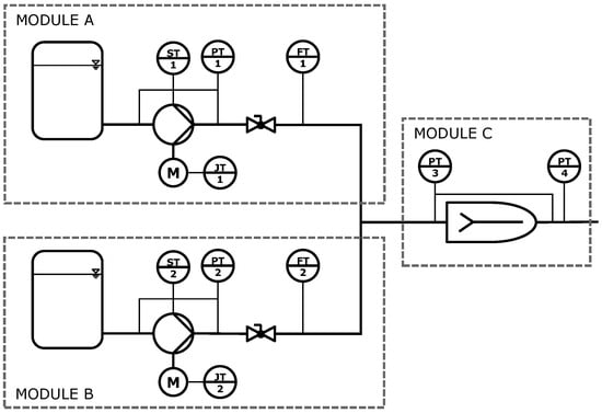
Figure 1.
A simplified plant consisting of two parallel dosing modules (A and B) that feed one mixing module (C). Measurement equipment for the electric motor power (JT), pump speed (ST), differential pressure (PT) and volume flow (FT) is installed for monitoring and validation purposes.
The volume flow exiting dosing modules A and B is subsequently conveyed through the mixing module C. Pressure losses within the dosing modules, such as those across the hand valves and mixers, vary with the volume flow. This behavior allows for the implementation of several observers that redundantly estimate the volume flow in the respective modules. In the dosing modules, the pump observers calculate the volume flow based on the pump speed and the differential pressure. Depending on the pump type, different models can be used. In the case of a progressive cavity pump, for example, it is
The power observer , on the other hand, utilizes measurements of the electric motor power and differential pressure to provide an alternative estimation of volume flow. The losses within the pump and its motor are represented by the efficiency , which depends on the differential pressure rotational speed:
The plant observer utilizes the pressure loss within the module to calculate the volume flow with the plant model parameters and :
For the mixing module C, observer values for the plant, power, and pump observer are calculated by summing the corresponding observer values from the upstream dosing modules. Additionally, module C features an independent plant observer referred to as the resistance observer , which uses the measured pressure loss across the mixing module to determine volume flow. The different observers redundantly calculate the volume flow. By comparing these observer values, residuals are generated as the differences between the outputs of different observers. This procedure is an expansion on the parity equations since the model output is not compared to a measured variable but to another model output. Further details can be found in [8].
The thermophysical properties of the conveyed fluid are temperature dependent and, consequently, influence the system dynamics captured by the observer models. Variations in fluid temperature, which can be reliably measured in the modules, must therefore be considered. Density and viscosity as functions of temperature are available in well-established databases, such as those provided by the National Institute of Standards and Technology [24]. The impact of fluid property variations on the observer models can be quantified. For instance, pressure loss in the plant observer can be described by the Colebrook–White correlation, which incorporates the Reynolds number and, hence, viscosity and density effects [25]. Analogously, the pump observer can be adapted following the modeling approach of Schänzle et al., which accounts for temperature-dependent behavior in the hydraulic performance of pumps [26].
Nevertheless, for the majority of applications in modular process plants, the temperature range of the fluids remains confined within narrow limits. Under such conditions, the observer models yield sufficiently accurate estimations even when simplifications regarding fluid properties are introduced.
3.1. Hydraulic Behavior
The module behavior for normal operation is illustrated in Figure 2. The pump characteristic shows a decrease in volume flow as the pressure difference increases. The plant characteristic, on the other hand, exhibits an increase in pressure difference with rising volume flow. Both characteristics intersect at the operating point, where both the pressure difference and the volume flow are defined. The aforementioned observers use the pressure difference to calculate the volume flow with the pump and plant model. For normal behavior, both will return the same value .
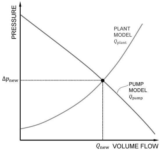
Figure 2.
In normal operation, the pump model and the plant model intersect at the operating point. Both observers calculate the same volume flow for the measured pressure.
In the presence of a fault, however, the behavior shifts, as depicted in Figure 3. The left panel shows the effects of pump wear resulting in internal leakage, while the right panel demonstrates the consequences of clogging within a module.
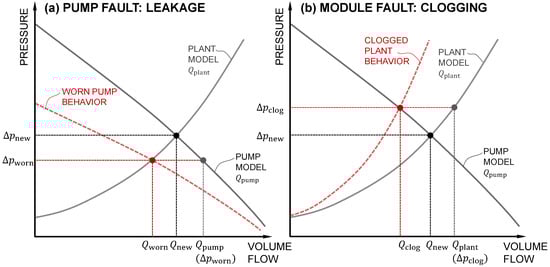
Figure 3.
Left: For the pump fault leakage, the pump characteristic is lower than before, shifting the operating point toward lower pressure and volume flow. Right: If the module is clogging, the pressure difference is rising and the operating point is at a lower volume flow.
When a pump experiences wear resulting in internal leakage, it is unable to maintain the same volume flow at a given pressure difference. This shifts the pump characteristic curve downward, resulting in a new operating point characterized by the lower volume flow and the lower pressure difference . With the reduced pressure difference as an input, the plant observer accurately calculates the volume flow . However, the pump observer—interpreting the lower pressure difference as indicative of a higher flow—overestimates the volume flow to . This discrepancy yields a positive residual .
Another fault is depicted on the right side of Figure 3. If the module is clogging, the pressure loss increases for a given volume flow. This shifts the operating point to a higher pressure and a lower volume flow . The pump observer, using the increased pressure difference, correctly estimates the volume flow as . However, the plant observer—still assuming normal module conditions—overestimates the flow as . This results in a negative residual .
These considerations are extended to all residuals and across all modules. The power observers exhibit similar behavior to the respective pump observers, as both are centered on the phenomena within the pump. Residuals unaffected by faults should ideally remain close to zero. However, residuals of the mixing module C, which is downstream of the faulty module A, will exhibit changes because the observers of module C aggregate the values from the upstream dosing modules. Consequently, any overestimation or underestimation by the observer of a faulty upstream module, such as module A, will propagate through to the mixing module, thus affecting its residuals.
3.2. Examined Faults
Various faults can occur in the simplified plant of Figure 1, each necessitating an effective quantification. For this purpose, the fault degree is defined. Here, the authors adopt the loss of functionality as a suitable representation of the fault degree, as it reflects the effect of each fault on the module performance. In detail, this means that the fault degree for each fault is defined as follows.
3.2.1. Leakage
As pumps wear over time, increased sealing gaps can lead to internal leakage, impacting their volumetric efficiency. To quantify this degradation, the fault degree is represented as the relative reduction in volumetric efficiency. This is derived by comparing the volume flow of the pump in a reference state without additional leakage, denoted as , to the actual volume flow under identical operating conditions. This comparison yields a fault degree , which is calculated as follows:
3.2.2. Module Clogging and Widening
Within dosing modules, pipes and valves can accumulate residue, leading to constrictions, or experience wear that results in widening. For both scenarios, the fault degree is characterized by changes in pressure loss, capturing deviations from the reference module behavior. Specifically, the fault degree for clogging or widening is expressed as the relative increase or decrease in pressure loss when compared to the pressure loss of a reference module without such faults, , while experiencing the same volume flow:
3.2.3. Mixer Clogging and Widening
In static mixers, the presence of mixing elements within the housing allows for effective fluid blending. However, residues can accumulate on these elements over time, leading to clogging. Conversely, the continuous flow can cause abrasion, resulting in widening gaps within the mixer. To quantify these faults, the fault degree for mixer clogging or widening is defined by the relative change in pressure loss. This is determined by comparing the pressure loss across a reference mixer without faults to that of the current mixer operating at the same volume flow:
3.2.4. Sensor Fault (Linearity Fault)
Accurate plant monitoring depends on a suite of sensors, which are each susceptible to faults. Sensor faults can manifest as changes in the linearity of the sensor output, causing deviations in slope. This results in measured values that deviate either positively or negatively from the expected output. Such behavior is investigated across various pressure sensors and power meters. The fault degree for sensor faults is thus defined as the relative deviation of the measured value from the reference value :
3.3. Fault-Symptom Matrix
For each of these faults, the residuals of the different modules can be estimated following the methodology outlined in Section 3.1. The corresponding results are presented in the fault-symptom matrix in Figure 4. Each row represents a specific fault, with residuals categorized and color-coded as positive (green), negative (orange), or approximately zero (grey), allowing for a distinctive residual signature. The fault cases of Figure 3 can be found in the first and third rows of the first column. The unique residual patterns generated by each fault enable a reliable identification and differentiation between fault types, underscoring the utility of this approach for accurate fault diagnosis in modular process plants.
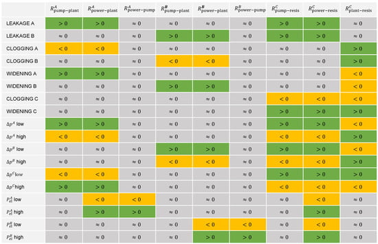
Figure 4.
Fault-symptom matrix for the examined faults in the simplified plant: The different faults (rows) result in values of the different residuals (columns) that are either positive, negative, or approximately zero. All lines are unique, meaning that there is a unique residual signature for every fault.
3.4. Derived Rules
The quantification of faults through general rules requires more than just an understanding of module interactions and fault degree definitions; it necessitates the linearization of the observer models for effective combination. These observer models, inherently based on quadratic equations and higher-order polynomials, are simplified through a Taylor series expansion truncated after the first-order term. This linear approximation, calculated at the current operating point, sufficiently captures the real behavior provided that deviations from the operating point remain small.
Each linearized model is defined by an offset c and a gradient m. The pump observer equation depends on the pump type. Considering the pump observer of a progressive cavity pump in Equation (1), the linearization at the operating point , and is therefore
with
and
Expanding upon the fault scenarios illustrated in Figure 3, and utilizing the defined fault degrees, general rules for fault quantification can be established. For pump leakage, the fault degree compares the actual volume flow with the volume flow of a reference pump without additional leakage. The actual volume flow is correctly estimated by the plant observer . The reference volume flow at the same pressure but without any pump faults is depicted by the pump observer . Therefore, the fault degree can be calculated:
Inserting the definition of the residual leads to
This rule defines the fault degree for pump leakage as a function of the calculated residual and observer values and can be used to quantify this fault.
For module clogging, as illustrated in Figure 3, deriving a quantitative relationship between the fault degree and the observed residuals requires a more nuanced approach. The fault degree for module clogging compares the actual pressure loss across the module with a reference without any clogging. The relationship between the fault degree and the residual can be derived as follows.
The calculation begins with the observer-estimated values of the volume flow. For a clogged module, the original volume flow under normal conditions, , is altered due to an increase in pressure loss, which is represented by the difference . The fault induces a shift in the operating point, and this shift affects both the pump and plant observer outputs. The linearized response of the system, captured by the observer gradients, enables us to express the residual in terms of the fault degree:
For the residual , this leads to
Inserting the definition of Equation (5) with and leads ultimately to
3.5. Rule Implementation
This method is applied for all residuals and all faults. By establishing relationships among all non-zero residuals corresponding to a given fault (see Figure 4), the approach integrates the (linearized) observer models, real-time measurements, and defined fault degrees. For a fault to be isolated and identified, all associated diagnostic rules must be fulfilled. This means that the unique signature of the residuals from Figure 4 is checked for each fault. This procedure is equivalent to a logical AND operation of the individual indicators.
Since all fault degrees are defined as positive, dimensionless quantities, the AND operation between the diagnostic rules can be realized using the minimum function. Consequently, the prevailing fault is identified as that fault for which the minimum of the associated fault degrees across all relevant residuals attains a maximum:
Here, denotes the detected fault, the set of all possible faults, and the set of relevant residuals.
The indicator calculation is implemented in a generalized framework. Depending on the fault type, the indicators for the residuals of the affected module and the parallel, up- and downstream modules are calculated. The necessary topological relationships are represented by an adjacency matrix, which encodes the relative positioning of all modules in the process plant. Adaptation of the fault diagnosis system to a different plant configuration is achieved solely by modifying the adjacency matrix. Thus, the diagnostic framework exhibits a high degree of structural flexibility and reusability.
The fault diagnosis system has been implemented in MATLAB and is publicly available (see data availability statement). The authors have developed the complete codebase, ensuring compatibility with the uncertainty propagation methods detailed in Section 3.6. This implementation provides a robust foundation for accurate and reliable fault diagnosis, accommodating the nuances of modular process plant operations while also accounting for measurement, parameter, and model uncertainties.
3.6. Uncertainty Quantification
The proposed methodology calculates a prognosis for different faults. It is based on measurements, model parameters, and model equations. All of these are uncertain, as models are merely a reflection of reality. To achieve trust in the results, the influence of the uncertainty has to be quantified [27].
3.6.1. Measurement Uncertainty
The measurements that are conducted are subject to uncertainty. The systematic uncertainty of the different measurement equipment is displayed in Table 1. All sensors are operated with a sampling rate of . The calculated values for the observers, residuals, and symptoms are only of interest on a larger timescale. Therefore, temporal averaging of the measured values is applied with a resolution of . The statistical and systematic uncertainties are combined using the case of uncorrelated input quantities; cf. the Guide to the Expression of Uncertainty in Measurement (GUM) [28]. Furthermore, uncertainty propagation is conducted accordingly.

Table 1.
Sensors on the test rig (FS: full scale; MV: measured value).
3.6.2. Parameter Uncertainty
All observers rely on model parameters such as and in Equation (1). To obtain these parameters, calibration measurements were performed. Meaningful datasets were measured through the targeted variation of the operating points (pressure difference and speed). The resulting measurement data were fitted to the model equations. Since no model fits the data perfectly, the best solutions derive from the least squares method, which seeks to minimize the distance of each measurement point from the model. The remaining deviation is a measure of the uncertainty of the model parameters [29]. For the presented validation results in Section 4.3, the model uncertainty remained low with a coefficient of determination of the model equations of at least .
3.6.3. Model Uncertainty
The proposed methodology also utilizes linearized observer equations. Through linearization of the (uncertain) model (c.f. previous subsection), additional uncertainty is introduced. The further the actual operation point is from the linearization point, the larger the additional model uncertainty. For this purpose, a conservative estimation was used that calculates the possible deviation in the gradient of the linearized models due to the prognosed fault level.
3.6.4. Uncertainty Propagation
The different types of uncertainty are aggregated by means of Gaussian uncertainty propagation. Their influence on the observer values, residuals, symptoms, and prognosis depends on the individual uncertainties and the partial derivations for the respective relationships.
The uncertainty of the diagnosis is derived from the uncertainty of the results of the individual diagnosis rules. For a fault to be diagnosed, all its associated diagnosis rules have to be triggered. This logical AND operator is implemented as the minimum among the relevant calculated fault degrees (see Section 3.5). The associated uncertainty is also calculated as the minimum of the fault degrees including its uncertainty, which leads to the uncertainty bounds of the diagnosis:
3.7. Integration of the Approach into Modular Production
The proposed methodology has been specifically developed to meet the requirements of modular production systems. The model-based symptoms for each module are derived from manufacturer-provided knowledge on the behavior of a module and parameterized by a limited number of measurements. Since each module remains unaltered after manufacture, the modeling effort is contained and highly manageable. The integration of the observers and symptom generation into the module automation can be performed by the module manufacturers without knowledge of the plant topology.
The central diagnosis system, however, is based on the plant operator’s knowledge of the plant topology and the interactions between modules within that topology. This operational understanding is distilled into a set of generalized diagnostic rules that can be efficiently applied to any given plant configuration. Consequently, the adaptation of the diagnosis system after the modular plant is reconfigured is minimal, thereby enhancing the adaptability and flexibility inherent to modular process plants.
4. Validation
The described methodology was experimentally validated using the test rig illustrated in Figure 5. This setup is specifically designed to simulate a variety of fault conditions and provides the necessary measurement data for comprehensive diagnosis and validation. For the scope of this study, a single fault scenario was chosen for detailed investigation. In this scenario, all previously outlined steps of the methodology were applied and thoroughly examined to evaluate the proposed approach. A range of different faults were also investigated in further studies. The overall results can be found in Section 4.3.
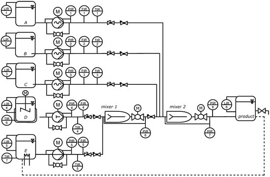
Figure 5.
The test rig is a modular mixing plant consisting of five dosing modules that feed two consecutive mixing modules.
4.1. Test Rig: Modular Mixing Plant
The test rig employed in this study is a modular mixing plant consisting of five dosing modules and two mixing modules. The dosing modules A, B and C convey fluids by means of progressive cavity pumps, while module D employs a membrane pump and module E utilizes a centrifugal pump. Each dosing module is equipped with sensors for the pump pressure, pump speed, and electrical power at the motor input. The volume flow exiting the dosing module is measured for validation purposes. There is a bypass installed parallel to each pump. If opened, the bypass allows a volume flow from the pressure to the suction side of the pump, simulating internal leakage in the pump.
The mixing modules consist of a static mixer and a valve that is normally open. It can be closed to replicate the fault of mixer clogging. The pressure loss across the whole mixing module is measured with a differential pressure sensor. Detailed specifications of all sensors used, along with their associated systematic uncertainties, are presented in Table 1.
The test rig is operated by the real-time rapid-prototyping system Microlabbox from dSPACE. It is equipped with a real-time interface for MATLAB/Simulink R2023a for model-based I/O integration and the experiment software ControlDesk 7.6. In this way, predefined operating scenarios (see the next section) were implemented, and all measurements were processed and saved with their accompanying metadata (see the data availability statement).
4.2. Scenarios
Different faults were experimentally simulated at the test rig. The details of these experiments can be found in Table 2. For each scenario, different fault degrees were implemented and held for approximately 10 s. This way, many stationary operating points with different fault degrees could be examined.
Table 2.
Experimental implementation of the different faults.
The following investigation examines internal pump leakage in module A, which is simulated by gradually opening the bypass valve. The corresponding valve opening angle is shown in the top panel of Figure 6. Due to hardware limitations, the valve opening must be adjusted in discrete increments, leading to the characteristic sawtooth profile observed. As the bypass valve opens further, a larger proportion of the flow is redirected to the suction side of the pump. This causes a reduction in the volume flow exiting the module, which is depicted in the bottom panel of Figure 6.
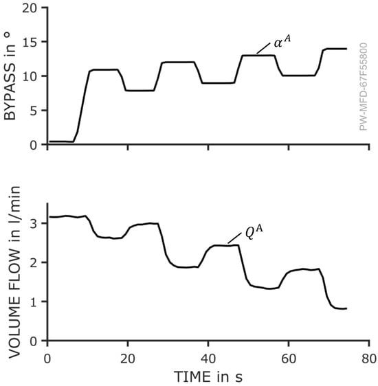
Figure 6.
Top: Pump leakage is simulated by opening the bypass in module A. Different degrees of bypass opening correspond to different fault degrees. Bottom: As the bypass opening increases, the effective volume flow rate discharged from the module diminishes accordingly.
In practice, internal pump leakage tends to increase progressively as a result of wear. Thus, the quasi-stationary wear states, represented by the plateaus of similar volume flow, correspond to distinct fault levels, which should be detected. The measurements during transitional phases, where rapid changes in the module condition occur, are of minor relevance for the analysis.
4.3. Results
The results for every step of the methodology are presented in the following section. The measured volume flow and the calculated observer values for the affected module A are shown in the top panel of Figure 7. The measured volume flow is gradually decreasing, and the measurements exhibit minor uncertainty. The plant observer closely tracks the real volume flow with small uncertainty. In contrast, the pump observer and power observer maintain relatively constant values, indicating that they are unaffected by the bypass opening. Since the pump continues to convey the same volume flow, these observers do not register the portion of the flow recirculating through the bypass rather than exiting the module. The uncertainty of the observers and residuals is portrayed by the shaded areas around the lines. Notably, the power observer portrays a significantly higher uncertainty than the uncertainty of the other observers, which is attributed to the higher systematic uncertainty of the power meter (see Table 1).
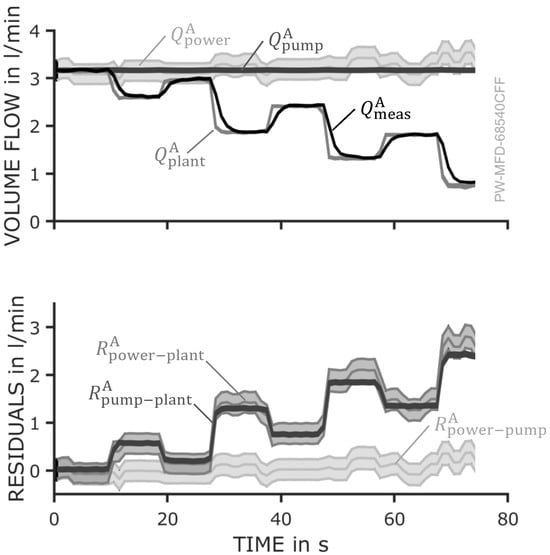
Figure 7.
Top: The measured volume flow is decreasing and correctly estimated by the plant observer. The pump and power observer estimate a constant volume flow with different uncertainty. Bottom: The residuals are as expected. Residuals and , rise and residual is approximately zero.
The residuals, plotted in the lower panel of Figure 7, represent the differences between the respective observers. With increasing leakage, the residuals and rise steadily, as the plant observer detects the reduction in volume flow that the pump and power observers fail to capture. Meanwhile, the residual between the power and pump observers remains near zero, as both consistently register the same (incorrect) volume flow value. This aligns with the expected behavior under this fault condition (see Figure 4).
For a further analysis and identification of the occurring fault, the residuals of all other modules have to be examined as well. Figure 8 illustrates the residuals of the parallel module B (top) and the downstream mixer 2 (bottom). The observers associated with the parallel module remain unaffected by the leakage in module A, as they calculate the actual volume flow for module B within their respective uncertainties. As a result, the differences between the observer values, as reflected in the residuals and their uncertainty interval, are nearly zero. In Figure 8, the uncertainty of and is considerably larger than that of . Therefore, the threshold for the classification of said residuals as is also larger to accommodate for the higher uncertainty. In contrast, the observer values for the downstream mixer 2 are influenced by the observer values of all preceding modules. The pump and power observers of mixer 2 aggregate the values from all prior pump and power observers, thereby propagating the erroneous values from module A. However, the resistance observer for mixer 2 operates independently, which is based on the differential pressure across the mixer. It effectively detects the decreasing volume flow caused by the internal leakage in module A. As a result, the residuals and increase as the fault severity escalates.
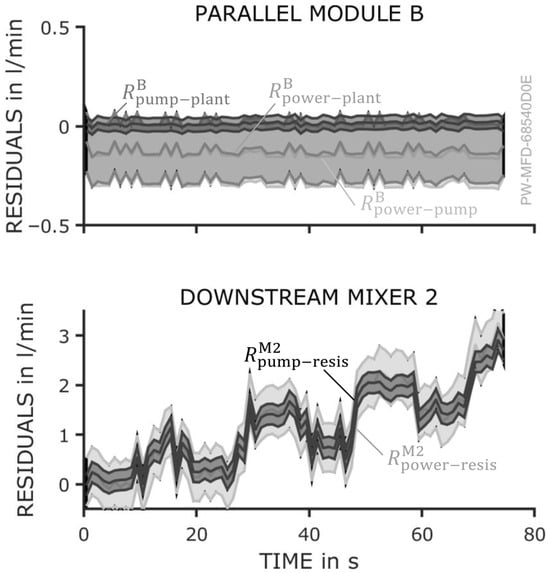
Figure 8.
Top: The parallel dosing module B is not affected by the pump fault in module A. Consequently, all residuals are zero. Bottom: The downstream mixing module M2 adds up the observer values including the faulty values of module B. Thus, residuals and increase.
The behavior of all residuals aligns with the expectations in Figure 4. The first row of the table indicates the different residuals for the fault “internal leakage” in module A. The residuals of the affected module and should exhibit an upward trend, while the residual remains unchanged. Residuals for the parallel module are expected to remain unaffected altogether. For the downstream module, residuals and increase, while residual remains unaffected.
To quantify the fault, the derived diagnostic rules (see Section 3.4) were applied and evaluated. The results are presented in Figure 9. The top panel illustrates the actual fault magnitude, which corresponds to the loss of functionality in the dosing module, specifically the reduction in volumetric efficiency. The bottom panel displays the diagnosed fault degree and its uncertainty over time.
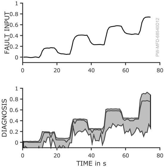
Figure 9.
Top: The fault degree is calculated according to the volume flow measurements. It is increasing and decreasing in a sawtooth pattern corresponding to the bypass opening (see Figure 6). Bottom: The prognosed fault degree of the leakage as a result of the evaluation follows the real fault pattern.
The results indicate that the predicted fault values closely follow the overall trend of the actual fault. While the different fault levels are correctly identified, slight deviations are observed along the plateaus. During periods without leakage (e.g., 0–10 s and 20–25 s), the prognosis correctly indicates that there is no fault. For a more detailed comparison of the actual fault and the prognosis, the plot shown in Figure 10 provides further insight.
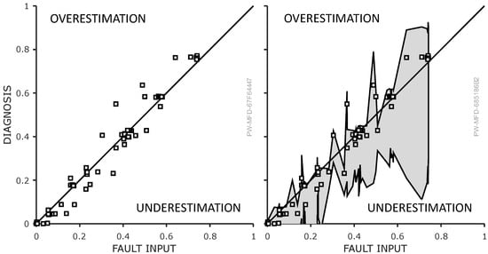
Figure 10.
Left: The prognosis is depicted over the actual fault. It shows that the prognosis is relatively close to the actual fault degree especially for operating points that were held for longer times. There is a slight underestimation. Right: The same diagram with the uncertainty of each prognosis shows that it diagnosed the fault correctly within its uncertainty.
Figure 10 plots the predicted prognosis over the actual fault degree for all time steps of the scenario (Figure 6). Stationary states, where the bypass valve maintains a constant opening and the fault level remains unchanged, are evident when multiple markers align vertically. Transitional states, where fault levels shift, are less significant for prognosis purposes but are nonetheless included in the diagram. The diagonal line signifies the ideal case, where the prognosis matches the actual fault level precisely.
The overall trend observed in the confusion matrix is promising. The markers are generally distributed along the ideal prognosis line, indicating a strong correlation between the actual fault degree and the predicted prognosis. The average absolute discrepancy between the diagnosed and simulated fault degree is 0.029. As the actual fault degree increases, the prognosis follows. Particularly at the fault levels of , and , where the system operates in a quasi-stationary state, the prognosis is in close agreement with the actual fault. These regions, characterized by a high density of markers, reflect the system’s performance under stable conditions. In contrast, deviations from the ideal line are more pronounced during transitions between fault levels. However, since the primary objective of the method is not to detect faults during these transient phases, these deviations are expected and not of significant concern.
The right-hand plot in Figure 10 presents the confusion matrix, including the associated uncertainty. The error bars are the result of the consistent uncertainty propagation as described in Section 3.6. At first glance, the uncertainty appears substantial—understandably so, as it arises from uncertain measurements and uncertain models with uncertain parameters. Additionally, the method applies conservative assumptions, further amplifying the perceived uncertainty. A closer inspection reveals an asymmetry in the error bars: the lower bounds are consistently wider than the upper bounds. This is a result of the uncertainty propagation as detailed in Section 3.6.4. Considering the uncertainty of the diagnosis, a fault is rather underestimated. However, the upper bounds of the uncertainty interval can be seen as a maximum fault degree. This underlines the method’s tendency to underestimate the fault magnitude as an inherent characteristic, stemming from its conservative nature.
Figure 11 presents the results of a comprehensive experimental evaluation involving single-fault scenarios across all modules of the modular mixing plant. The various fault types, as described in Section 3.2, were systematically introduced at over 1200 distinct stationary operating points. The discrepancy describes the difference between the diagnosis output and the actual fault degree. Each entry in Figure 11 indicates the frequency of occurrence for a given level of discrepancy at a specific fault degree.
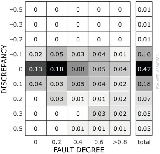
Figure 11.
Share of cases in a comprehensive study with faults in all modules and stationary operating conditions. The discrepancy is defined as the difference between the diagnostic results and the actual fault degree.
The results demonstrate that the proposed diagnostic system correctly identified the presence and approximate magnitude of the fault in the majority of cases with only minor deviations. Notably, larger discrepancies were observed primarily at higher fault degrees. The average absolute discrepancy between the diagnosis and the simulated fault degree is 0.12. Overall, the system exhibited a consistent tendency to underestimate fault severity, which is indicative of a conservative diagnostic behavior.
A review of scenarios with no faults also showed no diagnostic results. For the examined scenarios with single faults, there were also no diagnostic outputs as long as there was no fault simulated. This means that the diagnosis system triggered no false alarms, which reinforces confidence in the method’s reliability.
5. Discussion
The results presented in this study provide essential insights into the different stages of the proposed methodology. The different observers reliably calculate the volume flow for each module. The resulting uncertainty relates to the quality of the underlying models and the measurement equipment. The observer values align with the expected module interaction, allowing for the utilization of generalized rules for the fault diagnosis. As a result, the prognosis detects and identifies the correct fault with estimated fault magnitudes closely approximating the true values. Importantly, the system avoids false alarms, underscoring its robustness.
A quantitative comparison of the present experimental validation with alternative diagnostic methods proves difficult. The implementation and evaluation of diverse fault diagnosis algorithms are beyond the scope of this proof of concept and remain reserved for subsequent publications. Nevertheless, the complete experimental dataset is made publicly available. The authors explicitly invite the research community to apply their own concepts to the same benchmark case and to report comparative results.
When set against the state of the art, the following picture emerges: numerous model-based approaches for fault diagnosis have been proposed, yet their validation is predominantly limited to simplified laboratory systems rather than to systems with the complexity of the modular process plant in this publication. Such plants, by their very nature, pose additional challenges, such as sparse data, reconfigurable structures, and evolving operating conditions. For instance, Theilliol et al. employ a residual generator based on analytical modeling to supervise a three-tank system [30], while Chetouani et al. apply an Extended Kalman Filter to an exothermic reaction [31]. Both groups report on the successful detection and isolation of all simulated faults. However, the systems investigated are of reduced complexity, and the number of considered fault scenarios is limited. Both studies also highlight the considerable process knowledge and implementation effort required for scaling these methods to more complex plants such as the one addressed in this work.
Investigations on more complex processes yield results closer to those presented here. Morales et al. report detection rates of up to 80% for faults in an industrial dryer using an improved Rao–Blackwellised particle filter [32]. Höfling et al. combine parameter estimation with parity-space approaches to monitor faults in a thermal pilot plant and obtain detection rates ranging from 70% to 100% depending on the fault type [33]. Fuente et al. apply parameter estimation for fault detection and diagnosis in a wastewater treatment plant; even their most effective algorithm generates both missed and false alarms for certain faults [34]. More recently, Du et al. investigated chemical reactors using residual signal generators in the form of functional observers. They report a detection limit of approximately 15% [35].
In summary, the achieved results are broadly comparable to those of published model-based methods. Yet, the comparability itself is inherently limited by divergent experimental setups, system complexities, and evaluation protocols. This underscores both the necessity and the challenge of establishing common benchmarks for fault diagnosis in modular process plants.
A significant aspect of the methodology is its incorporation of uncertainty quantification. For the observer values, the associated uncertainties reflect the quality of parameter estimation and the sensitivity of the model to particular measurements. Upon propagating this uncertainty through to the prognosis results, the error bounds become notably wide. This presents a challenge: while the prognosis value closely aligns with the actual fault, the high level of uncertainty complicates accurate fault quantification. Consequently, the confidence in the diagnosis is reduced. Future research must address the conservative nature of these uncertainty approximations, aiming to refine the methodology and reduce the uncertainty intervals.
The scope of the present investigation is limited to the diagnosis of single-fault events. However, technical systems in practical operation are frequently exposed to more complex fault constellations, including multiple simultaneous faults as well as gradual degradation processes. In such cases, an effective fault diagnosis system must not only detect the presence of multiple faults but also quantify them accurately. The authors are currently working on an expansion of the presented study to also address multiple simultaneous faults. Initial investigations indicate that the fault detection mechanism based on residual evaluation remains operative under the occurrence of multiple faults. Nonetheless, the interpretability of residual patterns, as illustrated in Figure 4, is partially compromised. This impairs fault isolation and identification, necessitating further methodological refinement. Three principal strategies for the extension of the diagnostic concept to multiple-fault scenarios are under consideration:
Sequential Fault Diagnosis: In the case of temporally successive fault events, a hierarchical diagnosis approach can be applied. The diagnostic system must detect, isolate, and identify the initial fault, incorporating its influence into the residual structure before proceeding to subsequent fault events. The fault-symptom matrix must be dynamically updated to account for the altered system response due to preceding faults.
Modeling of Frequent Fault Combinations: If empirical analysis reveals recurring combinations of simultaneous faults, these multi-fault cases may be explicitly modeled. The corresponding residual signatures can be integrated into the fault-symptom matrix, thereby enabling a targeted diagnosis of high-probability fault constellations.
Trade-off Between Robustness and Isolability: A fundamental challenge in multi-fault diagnosis arises from the antagonistic relationship between diagnostic robustness and fault isolability. While the inclusion of additional residuals enhances the discriminatory power of the fault-symptom matrix, it simultaneously increases sensitivity to disturbances. In multi-fault conditions, this sensitivity is exacerbated as residuals may be simultaneously influenced by several fault mechanisms. Hence, a parsimonious selection of diagnostic indicators is desirable. Techniques for residual minimization, such as Principal Component Analysis (cf. [11]), offer a potential avenue for reducing the dimensionality of the residual space without sacrificing diagnostic performance.
The integration of these strategies requires both theoretical formalization and empirical validation. Accordingly, an extended methodology and corresponding experimental results will be presented in future work.
The validation results highlight the potential of the proposed methodology for real-world application for the monitoring of modular hydraulic systems in modular process plants. There, each module is controlled by its own controller, which processes local sensor data. The observer models could be embedded in these controllers, and their results could be communicated to a central diagnostic system at the plant level. There, the generalized rules could be applied to obtain the fault diagnosis result.
Despite these limitations, the presented methodology offers a robust approach for fault prognosis in modular hydraulic systems. Crucially, it achieves this without relying on historical data or prior experience with the specific plant topology. The generalized nature of the approach makes it adaptable across various plant configurations, providing a systematic and scalable solution for real-time fault diagnosis. The results indicate that despite current limitations, this methodology represents a promising advancement for the real-time monitoring and diagnosis of modular systems.
6. Summary and Outlook
The results of this study confirm that the methodology first introduced by Wetterich et al. [8] can be effectively implemented for fault diagnosis in modular process plants. The model-based observers redundantly calculate volume flow with minimal deviation under normal operating conditions. In the presence of a fault, the residuals exhibit distinct reactions, allowing for generalizations. Through the definition of a fault degree, a fault model in the form of diagnostic rules was derived. Validation of this approach, particularly for internal pump leakage, demonstrated its reliability. Although additional fault types were analyzed and diagnosed successfully, they are not discussed within the scope of this paper. The overall results of the proposed methodology are comparable to other published diagnostic algorithms.
This approach addresses a critical gap in fault diagnosis for modular process plants, where operating data are often sparse and plant topologies frequently change. The concept of model-based symptoms on the module level can be easily applied to various process equipment. This adaptability suggests a promising framework wherein module manufacturers could integrate model-based observers directly into their modules. Plant operators could then leverage these symptoms in conjunction with the overarching plant topology to implement centralized diagnostics.
Current limitations of the methodology include its sensitivity to model uncertainty and its focus on single-fault scenarios. Further research should aim to dissect and mitigate the various sources of uncertainty that impact the prognosis. Additionally, expanding the methodology to handle the simultaneous detection and identification of multiple faults represents a significant opportunity to enhance its diagnostic effectiveness.
In summary, the authors have a positive outlook on the application of this approach to modular hydraulic systems in process plants, particularly in supporting the flexible and reliable production of fine and specialty chemicals. Although existing limitations highlight areas for future exploration, they also point to opportunities for refinement and development. The authors anticipate that these avenues of research will be explored in forthcoming publications, contributing to the advancement of modular production technology.
Author Contributions
Conceptualization, P.W. and P.F.P.; methodology, P.W.; software, P.W.; validation, P.W.; formal analysis, P.W.; investigation, P.W.; resources, P.F.P.; data curation, P.W.; writing—original draft preparation, P.W.; writing—review and editing, P.W. and M.M.G.K.; visualization, P.W.; supervision, M.M.G.K. and P.F.P.; project administration, P.F.P.; funding acquisition, P.F.P. All authors have read and agreed to the published version of the manuscript.
Funding
This work was funded by the German Federal Ministry for Economic Affairs and Climate Action (BMWK) within the scope of the HECTOR research project as part of the ENPRO 2.0 Initiative (funding code: 03EN2006A). We acknowledge the support of the Deutsche Forschungsgemeinschaft (DFG—German Research Foundation) and the Open Access Publishing Fund of the Technical University of Darmstadt.
Data Availability Statement
The data of all figures in this publication are available at https://tudatalib.ulb.tu-darmstadt.de/handle/tudatalib/4555 (accessed on 25 April 2025). The data presented in this study are available at https://tudatalib.ulb.tu-darmstadt.de/handle/tudatalib/4565 (accessed on 25 April 2025). The program code for this study is available at https://tudatalib.ulb.tu-darmstadt.de/handle/tudatalib/4564 (accessed on 25 April 2025).
Conflicts of Interest
The authors declare no conflicts of interest.
Nomenclature
The following variables are used in this manuscript:
| Bypass opening angle | |
| Pressure difference | |
| Efficiency | |
| c | Offset of the linearized models |
| Pump model parameter | |
| g | Arbitrary measurement variable |
| Resistance model parameter | |
| Plant model parameter | |
| l | Fill level |
| Fault factor for sensor faults | |
| m | Gradient of the linearized models |
| n | Rotational speed |
| Electric power | |
| Q | Volume flow |
| R | Residual |
| T | Temperature |
| V | Geometric pump volume |
| x | Fault degree |
References
- ZVEI; NAMUR; PROCESSNET; VDMA. Process INDUSTRIE 4.0: The Age of Modular Production On the Doorstep to Market Launch. Available online: https://www.zvei.org/fileadmin/user_upload/Presse_und_Medien/Publikationen/2019/Maerz/Status_Report_Modulare_Produktion_-_On_the_doorstep_to_market_launch/Statusreport_Process_INDUSTRIE_4.0-_The_Age_of_Modular_Production_19.02.19__8_.pdf (accessed on 23 May 2025).
- Modular Plants: Flexible Chemical Production by Modularization and Standardization—Status Quo and Future Trends. Available online: https://www.semanticscholar.org/paper/Modular-Plants-Flexible-chemical-production-by-and/ce34758cbf2fd23313e0b759267fc4e591aa1917 (accessed on 23 May 2025).
- Process Engineering Plants Modular Plants: Fundamentals and Planning Modular Plants; VDI: Beuth Verlag: Berlin, Germany, 2020.
- Zheng, L.; Chen, X.; Qu, J.; Ma, X. A Review of Pressure Fluctuations in Centrifugal Pumps without or with Clearance Flow. Processes 2023, 11, 856. [Google Scholar] [CrossRef]
- Isermann, R. Fault-Diagnosis Applications: Model-Based Condition Monitoring: Actuators, Drives, Machinery, Plants, Sensors, and Fault-Tolerant Systems; Springer: Berlin/Heidelberg, Germany, 2011. [Google Scholar]
- Kudelina, K.; Vaimann, T.; Asad, B.; Rassõlkin, A.; Kallaste, A.; Demidova, G. Trends and Challenges in Intelligent Condition Monitoring of Electrical Machines Using Machine Learning. Appl. Sci. 2021, 11, 2761. [Google Scholar] [CrossRef]
- Sharif, M.A.; Grosvenor, R.I. Process plant condition monitoring and fault diagnosis. Proc. Inst. Mech. Eng. Part E J. Process Mech. Eng. 1998, 212, 13–30. [Google Scholar] [CrossRef]
- Wetterich, P.; Kuhr, M.M.G.; Pelz, P.F. Model-Based Condition Monitoring of Modular Process Plants. Processes 2023, 11, 2733. [Google Scholar] [CrossRef]
- Beard, R.V. Failure Accomodation in Linear Systems Through Self-Reorganization. Ph.D. Dissertation, Massachusetts Institute of Technology, Boston, MA, USA, 1971. [Google Scholar]
- Venkatasubramanian, V.; Rengaswamy, R.; Yin, K.; Kavuri, S.N. A review of process fault detection and diagnosis. Comput. Chem. Eng. 2003, 27, 293–311. [Google Scholar] [CrossRef]
- Isermann, R. Fault-Diagnosis Systems: An Introduction from Fault Detection to Fault Tolerance; Springer: Berlin/Heidelberg, Germany, 2006. [Google Scholar]
- Young, P. Parameter estimation for continuous-time models—A survey. Automatica 1981, 17, 23–39. [Google Scholar] [CrossRef]
- Frank, P.M. Fault diagnosis in dynamic systems using analytical and knowledge-based redundancy. Automatica 1990, 26, 459–474. [Google Scholar] [CrossRef]
- Isermann, R. Process fault detection based on modeling and estimation methods—A survey. Automatica 1984, 20, 387–404. [Google Scholar] [CrossRef]
- Cimpoesu, E.M.; Ciubotaru, B.D.; Stefanoiu, D. Fault Detection and Identification Using Parameter Estimation Techniques. U.P.B. Sci. Bull. 2014, 76, 3–14. [Google Scholar]
- Chow, E.; Willsky, A. Analytical redundancy and the design of robust failure detection systems. IEEE Trans. Autom. Control 1984, 29, 603–614. [Google Scholar] [CrossRef]
- Omana, M.; Taylor, J.H. Robust Fault Detection and Isolation Using a Parity Equation Implementation of Directional Residuals. In Proceedings of the IEEE Advanced Process Control Applications for Industry Workshop (APC2005), Portland, OR, USA, 8–10 June 2005. [Google Scholar]
- Gertler, J. Analytical Redundancy Methods in Fault Detection and Isolation—Survey and Synthesis. IFAC Proc. Vol. 1991, 24, 9–21. [Google Scholar] [CrossRef]
- Kalman, R.E. A New Approach to Linear Filtering and Prediction Problems. J. Basic Eng. 1960, 82, 35–45. [Google Scholar] [CrossRef]
- Wendel, J. Integrierte Navigationssysteme; Oldenbourg Wissenschaftsverlag: München, Germany, 2007. [Google Scholar] [CrossRef]
- Willsky, A.S. A survey of design methods for failure detection in dynamic systems. Automatica 1976, 12, 601–611. [Google Scholar] [CrossRef]
- Li, R.; Olson, J.H. Fault detection and diagnosis in a closed-loop nonlinear distillation process: Application of extended Kalman filters. Ind. Eng. Chem. Res. 1991, 30, 898–908. [Google Scholar] [CrossRef]
- Liu, H.; Liu, D.; Lu, C.; Wang, X. Fault Diagnosis of hydraulic Servo System using the unscented Kalman Filter. Asian J. Control 2014, 16, 1713–1725. [Google Scholar] [CrossRef]
- National Institute of Standards and Technology. NIST Chemistry WebBook, SRD 69: Thermophysical Properties of Fluid Systems; National Institute of Standards and Technology: Gaithersburg, MD, USA, 2025.
- Zeghadnia, L.; Robert, J.L.; Achour, B. Explicit solutions for turbulent flow friction factor: A review, assessment and approaches classification. Ain Shams Eng. J. 2019, 10, 243–252. [Google Scholar] [CrossRef]
- Schänzle, C.; Jost, K.; Metzger, M.; Ludwig, G.; Pelz, P.F. ERP Positive Displacement Pumps—Experimental Validation of a Type-Independent Efficiency Model. In Proceedings of the 4th International Rotating Equipment Conference, Wiesbaden, Germany, 24–25 September 2019. [Google Scholar] [CrossRef]
- Pelz, P.F.; Groche, P.; Pfetsch, M.E.; Schaeffner, M. Mastering Uncertainty in Mechanical Engineering; Springer International Publishing: Cham, Switzerland, 2021. [Google Scholar] [CrossRef]
- Evaluation of Measurement Data—Guide to the Expression of Uncertainty in Measurement; Joint Committee for Guides in Metrology: Sèvres, France, 2008.
- Kamke, W. Der Umgang Mit Experimentellen Daten, Insbesondere Fehleranalyse, im Physikalischen Anfänger-Praktikum: Eine Elementare Einführung, 10., erw. aufl. ed.; Shaker: Aachen, Germany, 2014. [Google Scholar]
- Theilliol, D.; Noura, H.; Ponsart, J.C. Fault diagnosis and accommodation of a three-tank system based on analytical redundancy. ISA Trans. 2002, 41, 365–382. [Google Scholar] [CrossRef] [PubMed]
- Chetouani, Y. Fault detection by using the innovation signal: Application to an exothermic reaction. Chem. Eng. Process. Process Intensif. 2004, 43, 1579–1585. [Google Scholar] [CrossRef]
- Morales-Menéndez, R.; None de Freitas, N.; Poole, D. Real-Time Monitoring of Complex Industrial Processes with Particle Filters. Adv. Neural Inf. Process. Syst. 2003, 15. [Google Scholar]
- Höfling, T.; Deibert, R.; Hecker, O. Fault Detection of Flowrate and Temperature Control Loops using Estimated Parity Equations. IFAC Proc. Vol. 1995, 28, 193–198. [Google Scholar] [CrossRef]
- Fuente, M.; Vega, P.; Zarrop, M.; Poch, M. Fault detection in a real wastewater plant using parameter-estimation techniques. Control Eng. Pract. 1996, 4, 1089–1098. [Google Scholar] [CrossRef]
- Du, P.; Wilhite, B.; Kravaris, C. Model–based fault diagnosis for safety–critical chemical reactors: An experimental study. AIChE J. 2024, 70, e18565. [Google Scholar] [CrossRef]


Disclaimer/Publisher’s Note: The statements, opinions and data contained in all publications are solely those of the individual author(s) and contributor(s) and not of MDPI and/or the editor(s). MDPI and/or the editor(s) disclaim responsibility for any injury to people or property resulting from any ideas, methods, instructions or products referred to in the content. |
© 2025 by the authors. Licensee MDPI, Basel, Switzerland. This article is an open access article distributed under the terms and conditions of the Creative Commons Attribution (CC BY) license (https://creativecommons.org/licenses/by/4.0/).