Optimization Method for Hot Air Reflow Soldering Process Based on Robust Design

Abstract

The process design of hot air reflow soldering is one of the key factors affecting the quality of PCBA (Printed Circuit Board Assembly) component products. In order to improve the product quality during the design process, this paper proposes a robust optimization-based finite element simulation analysis method including significant influencing factor screening, robustness evaluation, robust optimization, and reliability verification for the reflow soldering process. The simulation model of the reflow soldering process temperature field based on experiments is constructed and validated. Sensitivity analysis is used to select important influencing factors, such as the last five set temperature zones (T5 to T9) in the reflow oven and the thermal properties of materials such as PCBs (printed circuit boards), BGAs (ball grid arrays), and solder paste, as well as noise factors like the heating environment during the soldering process. Several surrogate models are used to construct the response surface, and the optimal fitting scheme is selected to effectively avoid poor fitting caused by inappropriate surrogate models. The 6σ robust optimization approach is introduced to evaluate and optimize the robustness of the process design parameter where the heating factor is chosen as the optimization target. The reliability analysis method is employed to validate the product quality. This paper establishes a comprehensive robustness analysis method for hot air reflow soldering, effectively reducing design costs and addressing the lack of robustness analysis in the current hot air reflow soldering process design.

1. Introduction

With the trend of integration and miniaturization in electronic products, chip components have emerged, giving rise to the reflow soldering process, which quickly replaced the traditional manual soldering method in production processes. However, this advancement also brings complexity to process design and involves numerous influencing factors. As process technology continues to develop, high reliability and robustness have become the industry’s trends, especially in fields such as aerospace, aviation, and missile applications, where stringent operating environments require the precise design of the reflow soldering process window to meet high-quality soldering requirements. For most electronic products, the yield rate is the primary concern in the production process. Achieving high reliability and robustness in the reflow soldering process is crucial to ensure the optimal performance and functionality of electronic devices.

In most practical production processes, the process design commonly adopts a limited number of experiments and adjustments of process parameters, known as the “trial and error” method, to determine the optimal process parameters. However, this approach is inherently flawed, as it involves long design cycles and high costs. Additionally, it fails to account for the impact of uncertain factors such as material fluctuations and environmental loads, making it challenging to guarantee a high yield rate for products. In recent years, there have been numerous publications focusing on the analysis of the reflow soldering process. Esfandyari et al. [1] developed a simulation model using the finite element method to study the optimization relationship between process parameters, simulated thermal processes, and porosity in solder joints of a reflow oven under pressure. Khatibi et al. [2] conducted finite element simulations of PbSnAg solder using a stress rate and pressure-related material model to analyze its stress and strain states under static and cyclic loading conditions. Li Z.H. et al. [3] employed molecular dynamics to investigate the growth of intermetallic compounds (IMCs) between low-silver composite solders and copper substrates during the reflow soldering process. They explored the factors influencing copper atom diffusion rates, and explained the mechanisms behind the addition of CeOz nanoparticles in copper atom diffusion behavior and interfacial IMC growth. Long Xu et al. [4] improved the Coffin–Manson model and utilized the finite element method to predict the fatigue life of SAC305 solder joints under temperature cycling coupled with an electrical current. They revealed the performance advantages of lead-free solder with a high yield strength, and ultimate strength in the thermal fatigue and current density aspects. It is evident that there has been considerable research on reflow soldering, particularly in terms of reliability, in response to the trends of high reliability and robustness.

The current research on the robustness of reflow soldering processes is relatively limited and mainly relies on empirical or semi-empirical designs. Chowdhury et al. [5] utilized orthogonal experimental design to analyze the main factors causing variations in lead-free processes and optimized the solder wetting with the goal of achieving the best combination of strength through thermal cycling verification. Kung Chieh et al. [6] employed orthogonal experimental design to perform robust design analysis on the thermal-mechanical reliability of MCM (multi-chip module) packaging with flip-chip technology. They identified the substrate’s CTE (coefficient of thermal expansion) as the most significant factor influencing the reliability of coating fatigue and obtained the optimal combination parameters, resulting in a 554.5% increase in fatigue life under the best combination parameters. Chun-Sean Lau et al. [7] used the grey Taguchi method to optimize the thermal stress and cooling rate of BGA solder joints, determining the optimal parameter settings for multiple performance characteristics and validating the effectiveness of the optimization results through simulation experiments. Zhou Jicheng et al. [8] applied robust design and finite element methods, focusing on the thermal-mechanical fatigue life of solder joints. Considering eight control factors, they employed experimental design to optimize PBGA (plastic ball grid array) solder joints and obtained the optimal combination scheme. Tsai Tsung-Nan et al. [9] proposed a Taguchi method based on fuzzy logic to optimize the fine-pitch steel mesh printing process. They used multiple response optimization and analysis of variance (ANOVA) to determine the significant factors and compared the optimization performance with two hybrid methods. Sridhar Canumalla [10] introduced a response surface method to address advanced packaging reliability and robustness design issues. They described the descending life response function derived from the strain energy principle and presented a systematic approach to solve packaging reliability problems at the system level. Fupei Wu et al. [11] presented a robust positioning method for PCB solder joints, which offers higher precision and efficiency for smaller-sized positioning by eliminating uncertain factors. From the existing literature, it is evident that experimental design methods have been used to achieve robust design in reflow soldering processes. However, for aerospace electronic products with stringent requirements, the current methods still have significant limitations. Additionally, the influence of some important factors such as the temperature of the preheating zones and the material properties of the PCBA components on the robustness of the reflow soldering process have not been investigated, mainly due to the cost of the experimental design methods. Therefore, there is an urgent need for modern robust optimization methods that consider input fluctuations and ensure output consistency in the design of reflow soldering processes to meet the development trends of high reliability and robustness in electronic products.

This study adopts the 6σ criterion and considers the fluctuations in the temperature parameters of each zone in the reflow oven around their set values, as well as the influence of material characteristics’ fluctuations of PCBA components on the process. By selecting relevant influencing factors, a robustness evaluation module based on surrogate models and an embedded robustness optimization analysis module are constructed. This enables the automatic search for optimal robust design solutions, taking into account the impact of uncertain factors during the initial design stage. The proposed method offers a low-cost, efficient, and high-quality optimization approach, making it highly valuable for improving the yield rate in practical engineering applications.

2. Establishing Accurate Simulation Model

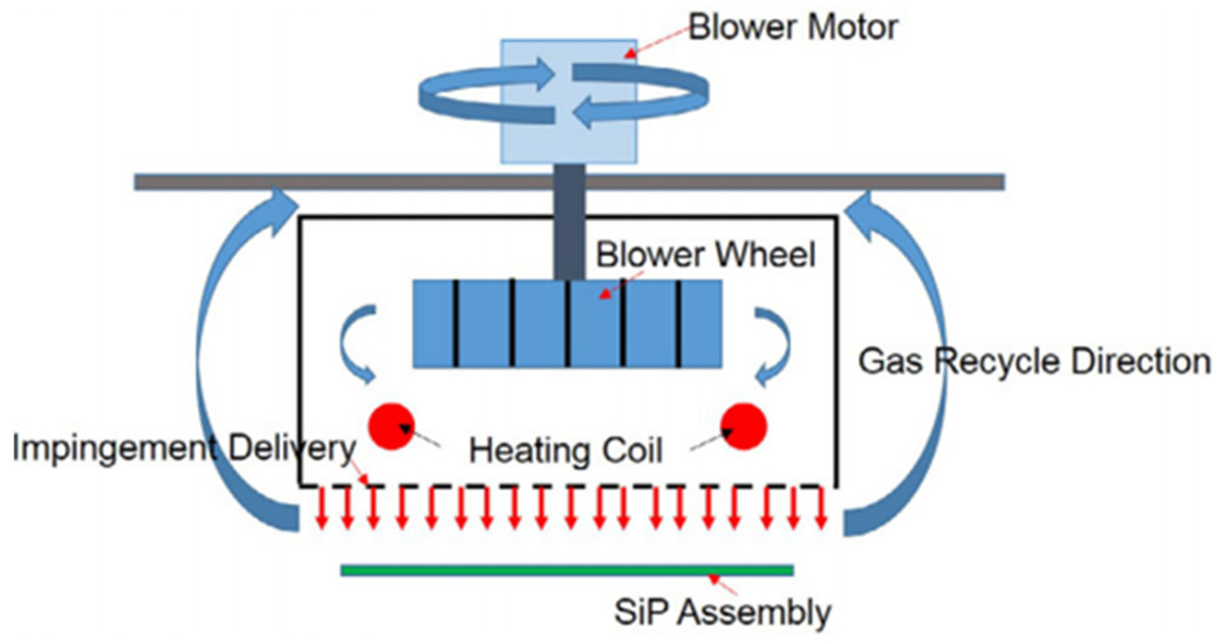
Reflow soldering, as one of the key processes in SMT (surface mount technology) production, directly affects the soldering quality and reliability of electronic products [12]. Its essence lies in the process of “heating”, which involves heating the air and using fans to deliver the heated airflow to the soldering surface. 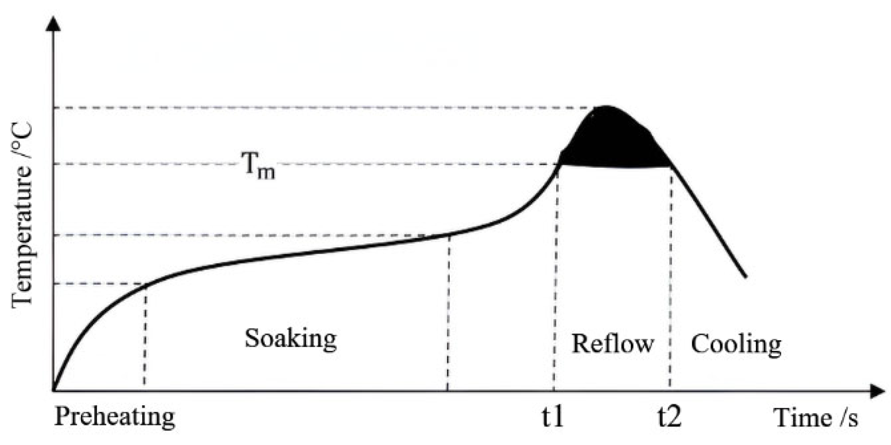This action melts the solder paste and forms solder joints between surface-mounted components and the PCB without altering the original characteristics of electronic components [13], as shown in Figure 1, the schematic diagram of the reflow soldering process. The core of this process involves designing temperature profiles and furnace temperature settings. The temperature profile refers to the “temperature-time” curve established for the representative packages and solder paste used in soldering PCBA. It also includes the “temperature-time” curve for testing points on the PCBA. Only within a reasonable process window can the product achieve high reliability. On the other hand, furnace temperature settings refer to the temperatures set by operators for each zone’s built-in thermocouples on the control panel, according to the designed temperature profile.

During the production process, the temperature profile at the solder joints is either equal to or fixed at a certain difference from the furnace temperature setting. As they are mainly influenced by factors such as the environment, materials, or structural dimensions, it is generally necessary to adjust process parameters through design. This includes temperature adjustments in various zones, conveyor belt speed, airflow, etc. [14] to achieve the appropriate process requirements and ensure a higher yield of good-quality products.

To establish an accurate simulation analysis of the reflow soldering process, this paper utilizes the Ansys Icepak finite element simulation module, which effectively addresses the inconsistency between the temperature profile at the solder joints and the furnace temperature setting. By designing the specified temperature, the simulation can obtain the desired temperature profile at the solder joints, allowing for an assessment of the rationality of process parameters. This approach omits the calculation of convective heat transfer coefficients during the intermediate process, thereby reducing the errors introduced in the intermediate steps.

This paper focuses on a specific model of hot air reflow soldering oven as the research subject. The main objective is to establish an accurate simulation model for the thermal field of the reflow soldering process. This is achieved through three steps: first, the actual dimensions of the reflow oven cavity are measured; second, an equivalent geometric model of the real PCBA components is created; and third, an equivalent thermal property parameter model is established. By addressing the challenges of measuring certain parameters, this approach enables the construction of a precise simulation model for the hot air reflow soldering process.

2.1. Reflow Soldering Oven Chamber Size

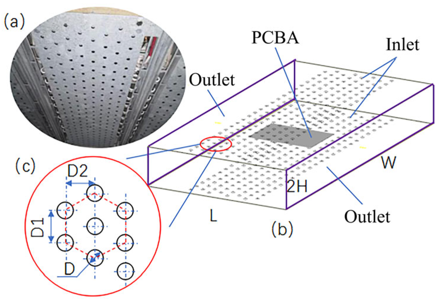
The reflow soldering oven has eight front heating zones and two rear cooling zones, with each zone having a transition area between them. As shown in Figure 2, based on actual measurements, the width of each individual reflow zone (W) is $W=630 \mathrm{m}\mathrm{m}$, the length (L) is $L=320 \mathrm{m}\mathrm{m}$, and the height from the outlet to the conveyor rail (H) is $H=45 \mathrm{m}\mathrm{m}$. Each circular nozzle has a diameter (D) of $D=7.5 \mathrm{m}\mathrm{m}$ and is arranged in a regular hexagonal pattern. The horizontal spacing (D1) between the nozzles is $D1=25 \mathrm{m}\mathrm{m}$, and the vertical spacing (D2) is $D2=12.5 \mathrm{m}\mathrm{m}$. The distribution of the oven cavity is consistent both vertically and horizontally. The experimental conveyor speed is set at $80 \mathrm{c}\mathrm{m}/\mathrm{m}\mathrm{i}\mathrm{n}$.

2.2. PCBA Component Equivalent Model

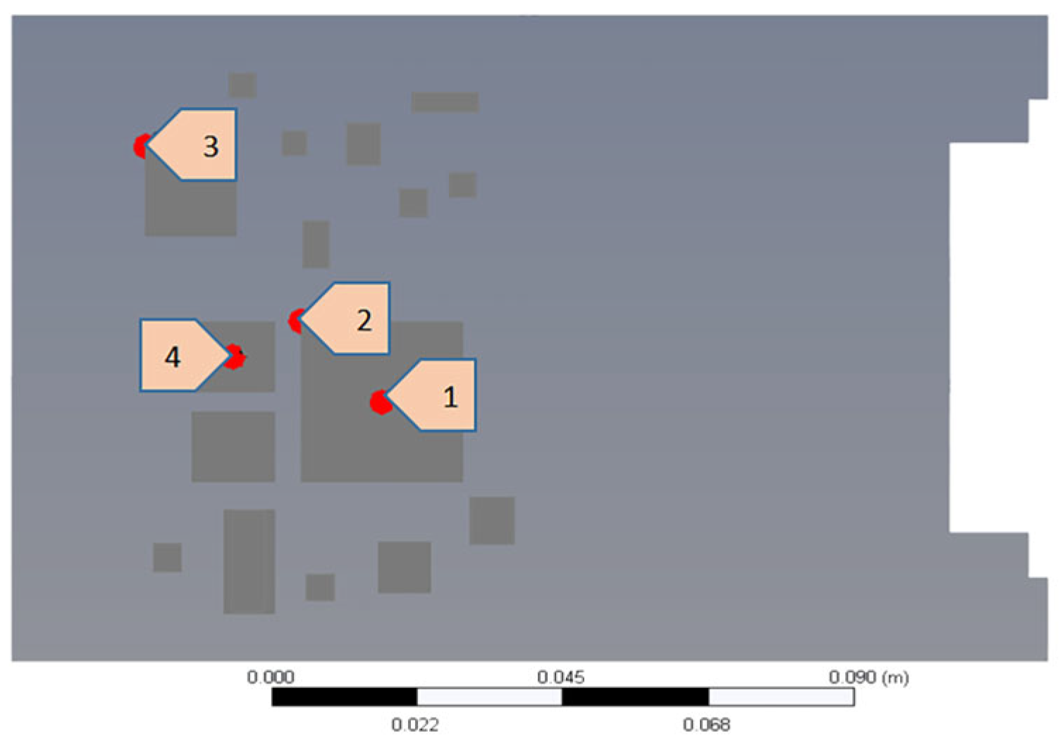
This experiment focuses on a specific PCBA produced by a certain manufacturer. The printed circuit board consists of a material substrate with copper foil for electrical interconnections. The board integrates various packaged components, including ball grid arrays (BGAs), chips, and resistors. An equivalent geometric model of the PCBA components based on the actual components is established for the research. Considering the precision requirements for smaller-sized components that have a minimal impact on the temperature field, they are either neglected or treated with a simplified approach. Complex components such as BGAs are simplified using a thermal resistance network model to obtain the simplified model, as shown in Figure 3, and the thermal material properties of each component are obtained and listed in

Table 1. Thermal properties of various materials.

Material	Density (kg/m3)	Specific Heat Capacity (J/(kg·°C))	Thermal Conductivity (W/m·°C)
Cu	8839	20 °C   356.8 80 °C   375.5 120 °C   388.0 160 °C   400.4 200 °C   412.8 225 °C   420.6 240 °C   425.3	20 °C   521.5 80 °C   532.0 120 °C   539.0 160 °C   546.0 200 °C   553.3 225 °C   557.7 240 °C   560.0
Substrate	1859	20 °C   1100 80 °C   1400 120 °C   1500 160 °C   1550 200 °C   1600 225 °C   1610 240 °C   1640	0.29
Solder paste Sn63Pb37	8218	196	50.2
Components	1800	40 °C   840 80 °C   850 120 °C   900 160 °C   960 200 °C   1000 225 °C   1050 240 °C   900	18

.

2.3. Parameter Correction

In Icepak simulation analysis, determining the temperature and airflow velocity of the nozzles is crucial. The temperature of the nozzles represents the set temperature, while the airflow velocity is a challenging parameter to measure accurately, yet it significantly affects the temperature field. To ensure the precision of the model within a deviation range of ±10 °C, establishing an accurate simulation model is essential. In the previous literature, the calculation of airflow velocity has been based on H. Martin’s formula [15]. However, this approach has certain limitations [16], and when applied to this experiment, it introduces considerable errors, as shown in Figure 4. The simulated curve exhibits poor fitting to the measured curve, indicating significant discrepancies.

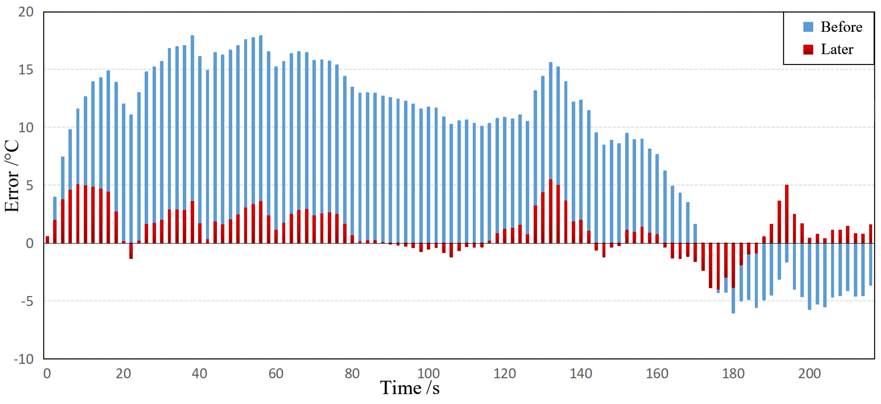
Therefore, this experiment adopts the method of temperature field correction based on established real measurement data, including four processes: building the reflow soldering process simulation model, determining the experimental design, constructing the response surface model, and optimizing and solving. Specifically, using aluminum alloy $2A12-H112$ plate as the test object, with the nozzle air velocity of 10 temperature zones as the variable, and minimizing the difference between the simulated curve and the measured curve at monitoring points as the objective, the optimized parameters of air velocity in each temperature zone are obtained through the response surface optimization method. The before and after correction, the error between the measured temperature curve and the simulated temperature curve is shown in Figure 5. It can be observed that the error before correction is mostly around 66.7% greater than ±10 °C, and even reaches nearly 20 °C at the maximum deviation. However, after correction, the error is mainly within the range of (−5, 5) °C, indicating a significant improvement in the correction effect.

To ensure the reliability of the correction results, the actual printed circuit board assembly component mentioned above was used as the validation object. By comparing the measured results of the PCBA component with the corrected simulation results, the accuracy of the correction effect was verified. The final results are shown in

Table 2. Parameters’ correction results for each temperature zone.

Temperature Zone	1	2	3	4	5	6	7	8	9	10
$\mathrm{Set} \mathrm{Temperature} (°\mathrm{C}$)	160	170	180	180	180	210	260	250	130	130
$\mathrm{Corrected} \mathrm{Result} (\mathrm{Wind} \mathrm{Speed}, \mathrm{m}/\mathrm{s}$)	15.37	14.21	11.59	11.50	11.06	6.02	5.04	7.07	6.88	2.51
$\mathrm{Max} \mathrm{Temperature} \mathrm{Difference} \ast \Delta 1 (°\mathrm{C})$	5.04	2.85	3.61	3.60	2.89	0.73	5.47	1.37	3.99	5.01
$\mathrm{Max} \mathrm{Temperature} \mathrm{Difference} \Delta 2 (°\mathrm{C})$	2.56	3.47	2.41	0.51	2.45	4.48	5.61	1.25	4.91	1.02

$\ast \Delta 1$ represents the maximum error between simulation and measurement for each temperature zone of the aluminum alloy plate. $\Delta 2$ represents the maximum error between simulation and measurement for each temperature zone of the printed circuit board.

. It can be observed that the temperature differences between the two simulations and the measurements are all less than 6 °C, thus meeting the accuracy requirement.

3. Parameter Selection Strategy Based on Sensitivity Analysis

3.1. Theoretical Basis

Sensitivity analysis is a technique that explores the extent to which the output responses of a system or model are influenced by changes in various input variables. It mainly includes local sensitivity analysis [17] and global sensitivity analysis [18]. Currently, mainstream global sensitivity analysis methods include the correlation coefficient method, the Morris filtering method, variance-based methods, etc. In this study, the variance-based global sensitivity analysis is adopted, specifically using a surrogate model-based approach. The fundamental idea is to construct an approximate mathematical model based on a set of training samples to replace the real model.

However, global sensitivity analysis based on surrogate models encounters two main sources of error: firstly, the approximation error of the surrogate model to the real model; secondly, the error arising from the low accuracy of the surrogate model leading to high-dimensional integration approximation. To enhance the accuracy of sensitivity analysis, this chapter adopts a method that connects the Icepak simulation analysis model with optiSLang data. Moreover, multiple surrogate models are selected for fitting, and the optimal fitting approach is determined based on the determination coefficient (R²) and the Coefficient of Prognosis (CoP) of each constraint and objective function.

3.2. Establishment of Optimization Objective

In the reflow soldering process, common process defects include solder voids, solder cracks, poor solder formation, and inappropriate intermetallic compound [19,20] thickness, among others. With the advancement of SMT, these common defects have been effectively controlled. However, for products with high reliability requirements, such as aerospace products, additional considerations need to be taken into account, including reliability and thermal fatigue life. These aspects cannot be rapidly identified, hence the need for early consideration during the process design phase. Based on existing research, it has been found that the thickness of the IMC significantly affects the reliability of solder joints [21]. Moreover, using the heating factor concept proposed by Professor Wu Yiping [22], a robust correlation has been established between the solder joint temperature curve and the IMC thickness, defined as follows:

$$Q_{\eta }={\displaystyle {\int }_{t1}^{t2}(T(t)-T_m)}dt$$

(1)

In the equation, $Q_{\eta }$ represents the heating factor, $T_m$ is the melting temperature of the solder alloy, and $t_1$ and $t_2$ are the start and end times when the reflow curve reaches $T_m$, respectively. Please refer to Figure 6, where the black region represents this timeframe.

The proposed heating factor is not necessarily better as it becomes larger (or smaller); rather, there exists an optimal range. Therefore, while aiming to ensure that all solder joints of the entire printed circuit board component fall within the optimal range of the heating factor, it is necessary to identify the most temperature-sensitive “hot spots” and the least temperature-sensitive “cold spots” on the printed circuit board component. By controlling the heating factor of the “cold spots” and “hot spots” within a favorable range, the optimization can be achieved. Based on the above analysis, this paper sets up monitoring points as shown in Figure 7, mainly analyzing the temperature curves of solder joints near the BGA and solder paste, and uses $Q_{\eta }$ as the optimization objective. Constraints are established according to the process requirements for Sn63/Pb37 solder paste reflow soldering, as shown in

Table 3. Objective and constraint settings.

Variables	Type	Range
$\mathrm{Cold} \mathrm{spots} Q_{\eta 1}, Q_{\eta 2}, Q_{\eta 3}, Q_{\eta 4} (°\mathrm{C}·\mathrm{s})$	Objective	Minimum
$\mathrm{Heating} \mathrm{factor} Q_{\eta 1}~Q_{\eta 4} (°\mathrm{C}·\mathrm{s})$	Constraint	800~1600
$\mathrm{Peak} \mathrm{temperature} T_{em} (°\mathrm{C})$	Constraint	210~230
$\mathrm{Time} \mathrm{above} \mathrm{liquidus} t_{eq} \left(\mathrm{s}\right)$	Constraint	60~90
$\mathrm{Soak} \mathrm{time} t_{eb} (°\mathrm{C})$	Constraint	60~90
$\mathrm{Cooling} \mathrm{rate} V_{ol} (°\mathrm{C}/\mathrm{s})$	Constraint	1.2~4

$Q_{\eta 1~4}$, respectively, represent the heating factors at the designated four monitoring points, with the point having the minimum heating factor referred to as the cold point. $T_{em}$ represents peak temperature, $t_{eq}$ represents time above the liquidus, $t_{eb}$ denotes soak time, and $V_{ol}$ signifies cooling rate.

.

3.3. Identification of Significant Influencing Factors

The above-mentioned objectives and constraints determine the noise factors and design variables. From the definition of the heating factor, it is known that the main factors causing changes in the heating factor are in the reflow zone, specifically the fifth to ninth zones (T5 to T9). Therefore, this study takes T5 to T9 as the optimized design variables. The noise factors that affect the heating factor of the solder joints mainly include the material thermal properties of the Sn63/Pb37 solder paste, the components, the BGA solder balls, the PCB, and the thermal properties of the environmental load nitrogen gas (N₂). This study considers the design errors and defects in various materials, as well as the facts that the reflow oven’s chambers are not completely isolated and the sides of the chambers have direct contact with the outside environment. As a result, the variable fluctuations were selected within the range of 1% to 5%. Using the Latin hypercube sampling method, a total of 100 simulations were performed to obtain the sample points and complete the sensitivity analysis of noise factor identification. The results of the analysis are shown in

Table 4. Quantitative analysis of material sensitivity to constraints and objectives.

Factors	Number	${\mathit{Q}}_{\mathit{\eta }\mathbf{1}} \mathbf{(}\mathbf{\%}\mathbf{)}$	${\mathit{Q}}_{\mathit{\eta }\mathbf{2}} \mathbf{(}\mathbf{\%}\mathbf{)}$	${\mathit{Q}}_{\mathit{\eta }\mathbf{3}} \mathbf{(}\mathbf{\%}\mathbf{)}$	${\mathit{Q}}_{\mathit{\eta }\mathbf{4}} \mathbf{(}\mathbf{\%}\mathbf{)}$	${\mathit{T}}_{\mathit{e}\mathit{m}} \mathbf{(}\mathbf{\%}\mathbf{)}$	${\mathit{t}}_{\mathit{e}\mathit{q}} \mathbf{(}\mathbf{\%}\mathbf{)}$	${\mathit{t}}_{\mathit{e}\mathit{b}} \mathbf{(}\mathbf{\%}\mathbf{)}$	${\mathit{V}}_{\mathit{o}\mathit{l}} \mathbf{(}\mathbf{\%}\mathbf{)}$
PCB Density	${\rho }_{pcb}$	28.2	27.9	25.5	27.3	27.5	25.1	9.5	28.9
PCB SHC	$C_{pcb}$	29.5	32.2	32.5	30.7	30.4	29.0	2.8	30.3
PCB Thermal Conductivity	$K_{pcb}$							2.8
N2 Density	${\rho }_{N_2}$	26.1	25.1	25.2	25.1	26.3	14.3	2.7	23.9
N2 SHC	$C_{N_2}$	15.4	13.1	14.0	14.6	14.9	9.2	6.4	15.1
N2 Thermal Conductivity	$K_{N_2}$
BGA Solder Ball Density	${\rho }_{BGA}$		0.6	1.3				2.8
BGA Solder Ball SHC	$C_{BGA}$						2.2	2.6
BGA Solder Ball Thermal Conductivity	$K_{BGA}$
Sn63/Pb37 Solder Density	${\rho }_{Sn-Pb}$				0.5
Sn63/Pb37 Solder SHC	$C_{Sn-Pb}$						5.5	6.1
Sn63/Pb37 Solder Thermal Conductivity	$K_{Sn-Pb}$

In the table, SHC is an abbreviation for specific heat capacity.

.

The sensitivity analysis above shows that the noise factors significantly affecting the objective function and constraint conditions include ${\rho }_{pcb}$, $C_{pcb}$, ${\rho }_{N_2}$, and $C_{N_2}$. This indicates that the PCB has the highest proportion in the entire PCBA assembly and is exposed to N₂ atmosphere during reflow soldering, which has a significant impact on the monitoring points. On the other hand, BGA solder balls and Sn63/Pb37 solder paste have smaller volumes, mainly influencing the temperature curves at their respective monitoring points. Based on these findings, ${\rho }_{pcb}$, $C_{pcb}$, ${\rho }_{N_2}$, and $C_{N_2}$ were selected as the noise factors.

4. Model Establishment of Surrogate Model

Due to the high computational cost of the original Icepak simulation model, as well as the consideration of noise factors and the influence of variable fluctuations in the subsequent robust optimization design, it is challenging to achieve. Therefore, a surrogate model was adopted to replace the original model [23].

4.1. The Method for Constructing the Surrogate Model

Unlike existing surrogate models constructed using certain approximation methods such as polynomial regression or kriging, this study utilized optiSLang with the Metamodel of Optimal Prognosis (MOP) proposed by Most and Will [24]. The fundamental idea of the MOP is to search for the optimal input variable set and the most suitable approximation model. It introduces an independent approach to evaluate the model quality, known as the Coefficient of Prognosis (CoP), which is defined as follows:

$$C\mathrm{o}P=1-\frac{S{S}_E^{\mathrm{Pr}ediction}}{S{S}_T}={\left(\frac{E\left[Y_{Test}·{\hat{Y}}_{Test}\right]}{{\sigma }_{Y_{Test}}{\sigma }_{{\hat{Y}}_{Test}}}\right)}^2$$

(2)

In the formula, $S{S}_E^{Prediction}$ represents the sum of the squares of the prediction errors; $S{S}_T$ represents the total change in output; $Y_{Test}$ represents the real output dataset; ${\widehat{Y}}_{Test}$ represents the output dataset predicted based on the meta-model; ${\sigma }_{Y_{Test}}$ and ${\sigma }_{{\widehat{Y}}_{Test}}$, respectively, represent the true and predicted variances. The measure $R^2$, which usually evaluates the approximate quality of the regression model, is defined as

$$R^2=1-\frac{S{S}_E}{S{S}_T}$$

(3)

The difference lies in the selection of the datasets. In simple terms, the calculation of the CoP values involves using data points that were not used to construct the approximation model. This means that the model quality is estimated only based on points that were not used in building the approximation model.

However, the MOP uses the prediction error rather than the fitting error, making it suitable for both regression and interpolation models. Moreover, to construct fast and reliable approximation models, linear or quadratic bases of polynomials or moving least squares approximation (MLS) were the preferred choices.

4.1.1. Polynomial Regression

Polynomial regression is a commonly used approximation method that has the advantages of simplicity in construction, low computational complexity, and fast convergence. The model’s response is typically composed of linear or quadratic polynomial basis functions, with or without interaction terms. Its basic theory is as follows:

$$y\left(x\right)=\hat{y}\left(x\right)+\epsilon$$

(4)

In the equation, $y\left(x\right)$ represents the actual response function, which is an unknown function. $\widehat{y}\left(x\right)$ represents the approximate function of the response, which needs to be obtained through fitting. $\epsilon$ represents the error between the approximation and the actual response.

As a polynomial response model, $\widehat{y}\left(x\right)$ is represented as

$$\hat{y}\left(x\right)=p^T\left(x\right)\hat{\beta }$$

(5)

where $p^T\left(x\right)$ is the polynomial basis function, defined as

$$p^T\left(x\right)=\left[\begin{array}{ccccccccc}1& x_1& x_2& \cdots & x_1^2& x_2^2& \cdots & x_1{x}_2& \cdots \end{array}\right]$$

(6)

The vector $\widehat{\beta }$ is a collection of unknown regression coefficients, obtained through fitting the model to a set of sample points, assuming independent errors and variances for each observation. Using matrix representation, the least squares solution is given using

$$\hat{\beta }={\left(P{P}^T\right)}^{-1}Py$$

(7)

where $P$ is the polynomial basis matrix containing the sample points, and y is the vector of sample point values.

4.1.2. Moving Least Squares (MLS) Approximation

In the moving least squares approximation, the local characteristics of regression were obtained by introducing position-dependent radial weighting functions. The basis functions can include any type of function, but typically only linear and quadratic terms are used. This basis function allows for an accurate representation by obtaining the best local fit to the actual interpolation points. The approximation function is defined as follows:

$$\hat{y}\left(x\right)=p^T\left(x\right)a\left(x\right)$$

(8)

To obtain the local regression model in the MLS method, a distance-dependent weighting function $\omega =\omega \left(s\right)$ was introduced, where $s$ represents the normalized distance between the interpolation point and the selected supporting point, given by using

$$s_i=\frac{\Vert x-x_i\Vert }{D}$$

(9)

where $D$ is the influence radius, defined as a numerical parameter. All types of functions can be used as the weighting function $\omega \left(s\right)$, and in most cases, the well-known Gaussian weighting function is employed:

$${\omega }_{\exp }\left(d\right)=\exp \left(-\frac{s^2}{{\alpha }^2}\right)$$

(10)

where $\alpha$ is a numerical constant, and the final approximation function is represented as

$$\hat{y}\left(x\right)=p^T\left(x\right){\left(P^{T}W\left(x\right)P\right)}^{-1}{P}^{T}W\left(x\right)y$$

(11)

where the diagonal matrix $W\left(x\right)$ contains the values of the weight function corresponding to $m$ support points.

$$W\left(x\right)=diag\left(\omega \left(d_1\right),\omega \left(d_2\right),\dots ,\omega \left(d_m\right)\right)$$

(12)

4.2. Establishing Response Surface

We selected appropriate variable ranges for the screened design variables. Due to considering subsequent response surface optimization analysis, some variable ranges needed to be appropriately expanded. Therefore, the variable ranges for T5~T9 were selected as follows: T5 (160–220), T6 (180–240), T7 (210–270), T8 (210–270), and T9 (80–150). The heating factor was chosen as the target value, with the reflow soldering process requirements as constraints, and considering the influence of noise factors. Through the established accurate temperature field simulation model, sample points were obtained using Latin hypercube sampling, and different proxy models were fitted using the above-mentioned methods. The quality of the approximate model was evaluated using the CoP and $R^2$, and a correlation analysis report was obtained. The proxy model with the highest fitting degree was selected to construct the response surface. The basic process is shown in Figure 8.

The results of response analysis are presented in

Table 5. Optimal metamodel results report.

Response	Type	Model	Variables	${\mathit{R}}^2$	CoP
$Q_{\eta }min$	Objective, Constraint	Kriging (Isotropic kernel)	9	0.999	0.995
$Q_{\eta }max$	Constraint	Kriging (Isotropic kernel)	9	0.999	0.995
$t_{eb}max$	Constraint	Kriging (Isotropic kernel)	2	0.951	0.939
$t_{eb}min$	Constraint	Kriging (Isotropic kernel)	2	0.929	0.904
$V_{ol}max$	Constraint	Linear Regression of order 1(no mixed terms)	7	0.983	0.983
$V_{ol}min$	Constraint	Linear Regression of order 1(with mixed terms)	9	1.000	0.999
$T_{em}max$	Constraint	Linear Regression of order 1(no mixed terms)	8	0.997	0.996
$T_{em}min$	Constraint	Linear Regression of order 1(no mixed terms)	8	0.994	0.993
$t_{eq}max$	Constraint	Kriging (Isotropic kernel)	9	0.989	0.952
$t_{eq}min$	Constraint	Kriging (Isotropic kernel)	9	0.982	0.942
$Q_{\eta 1}$	Objective	Kriging (Isotropic kernel)	9	1.000	0.997
$Q_{\eta 2}$	Objective	Kriging (Isotropic kernel)	9	0.999	0.995
$Q_{\eta 3}$	Objective	Linear Regression of order 1(no mixed terms)	9	0.981	0.980
$Q_{\eta 4}$	Objective	Linear Regression of order 2(no mixed terms)	9	0.988	0.985

In the table, “min” represents the minimum value of the variables, and “max” represents the maximum value of the variables.

. Since all constraints and objectives were ensured to be within the appropriate process window, it is necessary to consider the minimum and maximum values of each response.

4.3. Accuracy Verification

To ensure the accuracy of the response surface, it was necessary to perform accuracy validation on the constructed response functions. The specific approach involved comparing the optimization results based on the response surface with the results obtained from the original temperature field simulation model under the same parameters, ensuring that the error for each response was not greater than 5%. In this validation process, noise factors were not considered, and their values were set to fixed initial values. 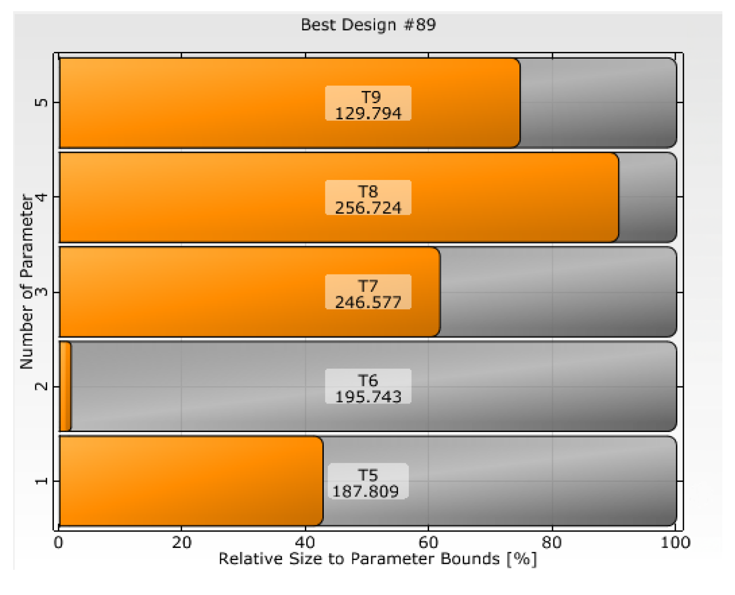Particle swarm optimization (PSO) [25] was employed for a quick local search on the response surface approximated using the proxy model. A gradient-based optimization module was constructed using the response surface, and the optimal set of temperatures for T5 to T9 was obtained, as shown in

Table 6. Optimization results based on response surface.

Process Parameters	Initial Design	Optimized Design
$\mathrm{T}5 (°\mathrm{C})$	180	183.3
$\mathrm{T}6 (°\mathrm{C})$	210	202.8
$\mathrm{T}7 (°\mathrm{C})$	260	239.4
$\mathrm{T}8 (°\mathrm{C})$	250	244.2
$\mathrm{T}9 (°\mathrm{C})$	130	122.5

T5~T9 represent the temperatures of the fifth to ninth temperature zones in the reflow oven.

.

Using the optimal set temperatures (T5~T9) obtained through the response surface optimization, we input them into the original temperature field simulation model to obtain the corresponding response values, as shown in

Table 7. Comparison of optimization results and original model simulation response values.

Constraints and Objectives	${\mathit{t}}_{\mathit{e}\mathit{b}} \mathbf{\left(}\mathbf{s}\mathbf{\right)}$		${\mathit{V}}_{\mathit{o}\mathit{l}} \mathbf{(}\mathbf{m}\mathbf{/}\mathbf{s}\mathbf{)}$		${\mathit{t}}_{\mathit{e}\mathit{q}} \mathbf{\left(}\mathbf{s}\mathbf{\right)}$		${\mathit{T}}_{\mathit{e}\mathit{m}} \mathbf{(}\mathbf{°}\mathbf{C}\mathbf{)}$		${\mathit{Q}}_{\mathit{\eta }} \mathbf{(}\mathbf{°}\mathbf{C}\mathbf{·}\mathbf{s}\mathbf{)}$
	Max	Min	Max	Min	Max	Min	Max	Min	Max	Min
Calculated	68	64	1.69	1.32	65.95	60.77	212.6	209.7	1055.2	973.4
MOP	68.1	62	1.76	1.32	66.26	60.23	212.8	210.0	1032.4	966.9
Deviation %	0.14	3.12	4.14	0	0.47	0.89	0.09	0.14	1.21	0.67

In the table, “Min” represents the minimum value of the variables, and “Max” represents the maximum value of the variables.

.

As shown in the table above, the deviations between the constraints and objectives obtained from the optimization based on the response surface and the simulation results of the original temperature field were all less than 5%. Therefore, the accuracy requirements were met.

5. Robust Optimization Design

Robustness refers to the insensitivity of the dependent variable (outcome or response) to small variations in the factors (causes or inputs). In simple terms, it involves analyzing the probability distribution of a product’s design standard. Robustness primarily focuses on the properties of the probability density curve near its mean, aiming to reduce sensitivity to variations in material properties and loads. This differs from reliability, which considers the tail properties of the probability density curve and requires the standard to be greater than the safety indicator. While these two concepts have differences, they also share certain connections.

5.1. 6σ Design Theory

To improve the yield of batch products, this study adopts the 6$\sigma$ robust design method, considering the influence of noise factors and control factor fluctuations on product quality. The concept of 6$\sigma$ originated from the field of quality engineering, and it refers to raising the probability of producing qualified products to a 6$\sigma$ level by measuring, analyzing, and controlling the impact of uncertainty factors on product quality [26,27]. The purpose of 6$\sigma$ design is to ensure that the mean of the objective function and design parameters still meet the constraint boundaries within the ±6$\sigma$ range, achieving a product qualification rate of up to 99.9999998%. Even with the wear of processing molds causing a deviation of 1.5$\sigma$ in product manufacturing accuracy, the defective rate is only 0.00034% [28].

Applying the robust design based on 6$\sigma$ to the reflow soldering process serves two main purposes: firstly, to analyze the robustness of batch products under a specific process scheme and establish a robustness evaluation module; secondly, to embed the robustness evaluation module into the optimization analysis model, constructing a robust optimization analysis module. Through automated optimization, the most robust process scheme was obtained. The basic definition is as follows:

$$\{\begin{array}{c}\min F=\pm {\mu }_f\left(x\right)+6{\sigma }_f\left(x\right)\\ s.t.G_j={\mu }_f+n{\sigma }_f\le B_{upper}\\ G_j={\mu }_f-n{\sigma }_f\ge B_{lower}\end{array}$$

(13)

In the equation, $x$ represents the design variables, $F$ represents the objective function, $G_j$ represents the constraint conditions, ${\mu }_f$ represents the mean of the response, ${\sigma }_f$ represents the variance of the response, and $B_{lower}$ and $B_{upper}$ are the lower and upper bounds of the constraint conditions.

5.2. Robustness Evaluation Module

The above fitted response functions were used to replace the original temperature field simulation model, and a robustness analysis module based on the response surface was constructed. Parameters such as noise factors ${\rho }_{pcb},$ $C_{pcb}$, ${\rho }_{N_2}$, $C_{N_2}$, and control variables T5~T9 were set with the parameter type, distribution type, and coefficient of variation (CoV). A total of 100 samples were generated using the ordinary Monte Carlo random sampling method to complete the initialization of the robustness assessment module. 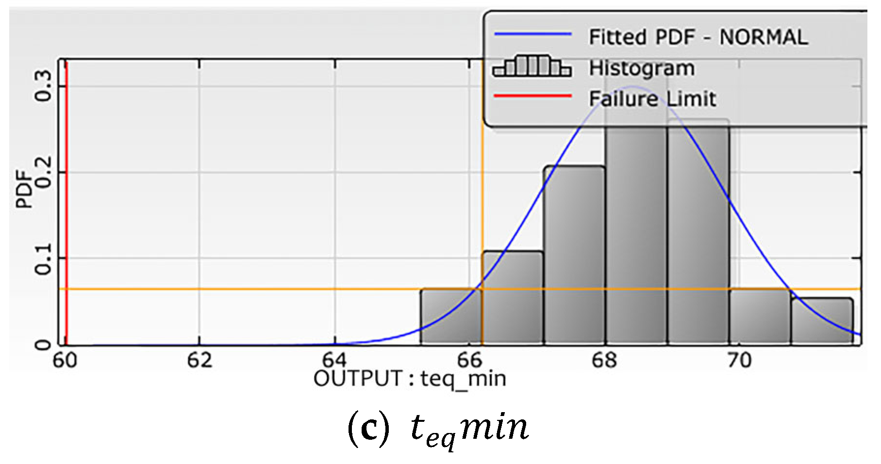By connecting the gradient-based optimization module with the robustness assessment module based on the response surface, the optimized process parameters (Table 6) were subjected to robustness evaluation. First, the cumulative distribution functions (CDF) of each response were analyzed to determine if they followed a normal distribution. Figure 9 shows the distribution of $Q_{\eta }min$.

It can be observed that the distribution function of $Q_{\eta }min$ is approximately normal, indicating that the probability distribution of $Q_{\eta }min$ follows a normal distribution. Similarly, the analysis shows that other constraint conditions also satisfy the normal distribution. The final results of the robustness evaluation are presented in Figure 10.

The specific $\sigma$ levels and failure probabilities are shown in

Table 8. Summary of $\sigma$ levels and failure probabilities for each response.

Response	Optimized Result	Mean	CoV	Failure Probability	$\mathit{\sigma }$ Level
$Q_{\eta }min$	966.9	962.46	0.0416	2.53 × 10−5	4
$Q_{\eta }max$	1032.4	1028.27	0.0409	0	13
$T_{em}min$	210.0	209.95	0.0034	0.52	0.06
$T_{em}max$	212.8	212.73	0.0034	0	23
$t_{eq}min$	60.23	60.15	0.0204	0.45	0.12
$t_{eq}max$	66.26	66.13	0.0229	0	15
$t_{eb}min$	62	61.88	0.0112	0	24
$t_{eb}max$	68.1	68.00	0.0114	0	28
$V_{ol}min$	1.32	1.32	0.0252	0	9
$V_{ol}max$	1.76	1.76	0.0243	0	52

Where CoV stands for coefficient of variation, and Mean represents the average or mean value.

.

From Table 8, it can be observed that although the mean values of the optimized process parameters based on the response surface optimization are close to the optimal values, and the maximum coefficient of variation (CoV) is relatively small, $Q_{\eta }min$, $T_{em}min$, and $t_{eq}min$ fail to achieve the 6$\sigma$ level. Additionally, $T_{em}min$ and $t_{eq}min$ have high failure probabilities and low $\sigma$ levels. Therefore, in the optimization design scheme, without considering noise factors and fluctuations in control variables in practical production, it may result in some products failing to meet the desired process requirements. When deviations are significant, the final outcome may lead to product failure.

5.3. Embedded Robustness Optimization Analysis Module

By embedding the robustness evaluation module into the newly established optimization analysis module, data interaction is achieved. The adaptive optimization method is employed to reconfigure the constraint conditions and complete the configuration of the optimization analysis module.

$$\{\begin{array}{c}obj.{\mu }_{Q_{\eta \min }}\to \min \\ s.t.{\mu }_{Q_{\eta \min }}-6{\sigma }_{Q_{\eta \min }}\ge 800\\ {\mu }_{Q_{\eta \max }}+6{\sigma }_{Q_{\eta \max }}\le 1600\\ {\mu }_{T_{e\mathrm{mmin}}}-6{\sigma }_{T_{\mathrm{emmin}}}\ge 210\\ {\mu }_{T_{e\mathrm{mmax}}}+6{\sigma }_{T_{\mathrm{emmax}}}\le 230\\ {\mu }_{t_{e\mathrm{qmin}}}-6{\sigma }_{t_{\mathrm{eqmin}}}\ge 60\\ {\mu }_{t_{eq\max }}+6{\sigma }_{t_{\mathrm{eqmax}}}\le 90\\ {\mu }_{t_{e\mathrm{bmin}}}-6{\sigma }_{t_{\mathrm{ebmin}}}\ge 60\\ {\mu }_{t_{e\mathrm{bmax}}}+6{\sigma }_{t_{\mathrm{ebmax}}}\le 90\\ {\mu }_{V_{o\mathrm{lmin}}}-6{\sigma }_{V_{\mathrm{olmin}}}\ge 1.2\\ {\mu }_{V_{o\mathrm{lmax}}}+6{\sigma }_{V_{\mathrm{olmax}}}\le 4\end{array}$$

(14)

The final result of the most robust solution is shown in Figure 11.

Analyzing the robustness of the optimization results, since the aforementioned $Q_{\eta }min,T_{em}min$, and $t_{eq}min$ did not reach the 6$\sigma$ level, the following mainly focuses on the robustness analysis of the responses $Q_{\eta }min,T_{em}min$, and $t_{eq}min$. The specific analysis results are shown in Figure 12 and

Table 9. Analysis of robust optimization results.

Response	Mean	CoV	Failure Probability	$\mathit{\sigma }$ Level (Robust Optimization)	$\mathit{\sigma }$ Level (Response Surface Optimization)
$Q_{\eta }min$	1180.34	0.0332	0	9	4
$Q_{\eta }max$	1244.11	0.0332	0	9	13
$T_{em}min$	209.95	0.0034	9.06 × 10−11	6	0.06
$T_{em}max$	217.4	0.0030	0	19	23
$t_{eq}min$	68.39	0.0195	1.55 × 10−10	6	0.12
$t_{eq}max$	73.54	0.0217	0	10	15
$t_{eb}min$	61.18	0.0144	0	18	24
$t_{eb}max$	67.86	0.0143	0	22	28
$V_{ol}min$	1.28	0.0234	0	9	9
$V_{ol}max$	1.76	0.0228	0	55	52

Where CoV stands for coefficient of variation, Mean represents the average or mean value.

.

From Table 8 and Table 9, it can be observed that the failure probabilities and $\sigma$ levels significantly improved through robust optimization. The failure probability for the supercritical fluid line time decreased from 0.45 to 1.55 × 10⁻¹⁰, while the $\sigma$ level increased from 0.12$\sigma$ to 6$\sigma$. Similarly, the failure probability for the peak temperature decreased from 0.52 to 9.06 × 10⁻¹¹, and the $\sigma$ level increased from 0.06$\sigma$ to 6$\sigma$. The results obtained from the robust optimization analysis demonstrate significant improvement in optimization performance, providing a substantial guarantee for the product’s yield rate.

5.4. Reliability Analysis and Verification

To verify the reliability of the optimized results and ensure that the influence of intermediate errors on the results is minimal, a reliability analysis was conducted on the results after robust optimization.

Firstly, a reliability analysis model was established to verify the intermediate errors. In this analysis, the reflow soldering process simulation model established in Chapter 2 was used as the original model. The noise factors and variables were reconfigured, and the extreme conditions and desired $\sigma$ levels of the process requirements were set to initialize the reliability analysis. The robust optimization module was then connected to the reliability analysis module, and the resulting data from the robust optimization were transferred to the reliability analysis module for further analysis.

By performing reliability analysis calculations, a reliability analysis report was generated. The report indicated that the embedded robust optimization response had reached a level of 5.7$\sigma$, with a failure probability of 8.6 × 10⁻⁹ and a standard deviation error of 5.1 × 10⁻⁹, thereby confirming the effectiveness of the optimization results. A scatter plot, as shown in Figure 13, was obtained for the input variables T5 and T8—peak temperature $T_{em}min$. The red areas in the plot represent the unsafe regions, clearly indicating the unsafe domain.

6. Conclusions

Reliability and robustness are important indicators for evaluating product quality. To ensure high product quality during the design phase, this paper focuses on the problem of yield uncertainty in the hot air reflow soldering process due to material, environmental, and design variable fluctuations. The 6$\sigma$ robust optimization approach is applied to the design of the reflow soldering process. A robust optimization design is achieved through the establishment of sensitivity analysis modules for identifying significant influencing parameters, a robustness evaluation module based on surrogate models, an embedded robustness optimization analysis module, and a reliability verification module. The specific advantages of the robust optimization design for the reflow soldering process are as follows:

• Precision control: This includes three aspects. First, a simulation model of the reflow soldering process temperature field based on experiments was constructed and validated through experiments to ensure the accuracy of the simulation model. Second, sensitivity analysis was used to select important influencing factors and avoid a rapid decrease in the quality of the approximate model with an increasing number of variables. Finally, multiple surrogate models were used to fit the objective function and constraint conditions, and the optimal fitting scheme was selected to effectively avoid poor fitting caused by inappropriate surrogate models, which could affect the final results.
• Establishment of robust optimization model: A robust optimization model was built with robustness evaluation indicators as constraint conditions, which allowed for automatic iteration to find the most robust solution. This effectively avoids the inefficiency and inaccuracy of manual iteration, reducing the design cycle.
• A complete robust optimization design method for the hot air reflow soldering process was established, including significant influencing factor screening, robustness evaluation, robust optimization, and reliability verification. It is a modern robust optimization method that considers input variability and ensures output consistency.