Design and Simulation of a Feedback Controller for an Active Suspension System: A Simplified Approach

Abstract

The concept of controlling vehicle comfort is a common problem that is faced in most under- and postgraduate courses in Engineering Schools. The aim of this study is to provide a simplified approach for the feedback control design and simulation of active suspension systems, which are applied in vehicles. Firstly, the mathematical model of an active suspension system (a quarter model of a car) which consists of a passive spring, a passive damper and an actuator is provided. In this study, we chose to design and compare the following controllers: (a) conventional P, PI and PID controllers that were tuned through two conventional methodologies (Ziegler–Nichols and Tyreus–Luyben); (b) an optimal PID controller that was tuned with a genetic algorithm (GA) optimization framework in terms of the minimization of certain performance criteria and (c) an internal model controller (IMC) based on the process transfer function. The controllers’ performance was assessed in a series of realistic scenarios that included set-point tracking with and without disturbances. In all cases, the IMC controller and the optimal PID showed superior performance. On the other hand, the P and PI controllers showed a rather insufficient behavior that involved persistent errors, overshoots and eventually, uncomfortable ride oscillations. Clearly, a step-by-step approach such as this, that includes modeling, control design and simulation scenarios can be applied to numerous other engineering examples, which we envisage to lead more students into the area of automatic control.

1. Introduction

One of the modern applications of automatic control technology in mobile applications is vehicle control (either with or without a driver) that ensures road-handling ability and ride comfort. One of these fascinating applications is the cruise control system that adjusts the car’s speed based on data received by a set of sensors and is implemented with advanced control techniques [1,2,3]. Another interesting area is lane-free control systems that use sensors and cameras to steer vehicles and retain them inside their lane without any action from the driver. Furthermore, the blind-spot-monitoring control system can detect when a car or a random object is out of sight. The latter can be combined with anti-collision warning control systems that warn the driver if such an obstacle is detected within the vehicle direction. Clearly, the above applications have received significant attention from researchers [4,5]. Still, however, the suspension control system, which is responsible for controlling and adjusting the ride comfort with an aim of reducing oscillations, is always at the forefront of research and lectures in engineering schools (mainly in undergraduate studies).

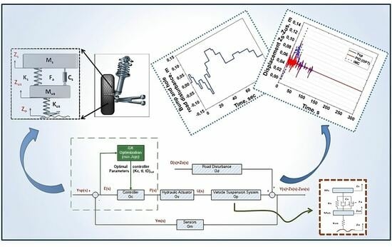
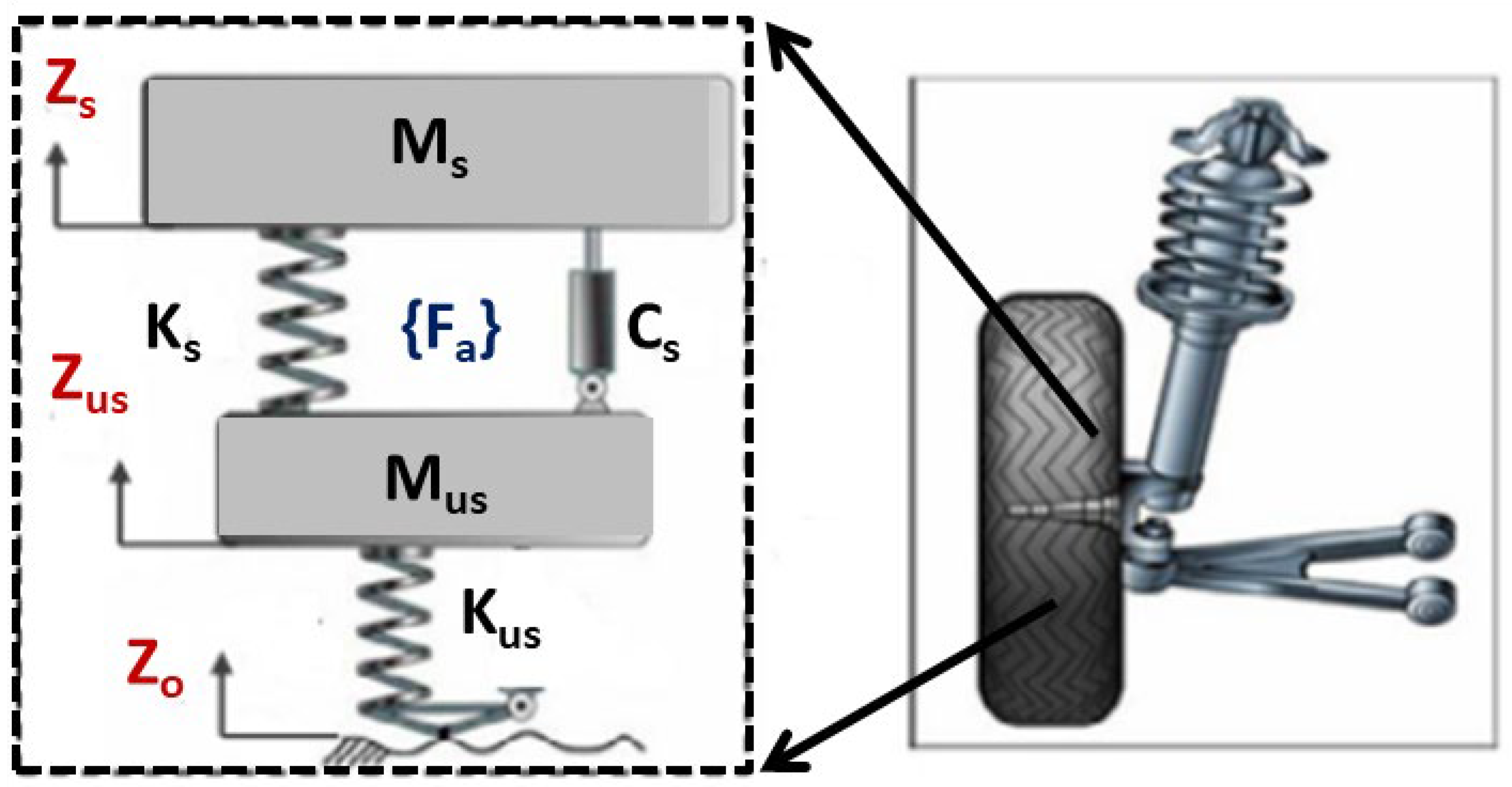
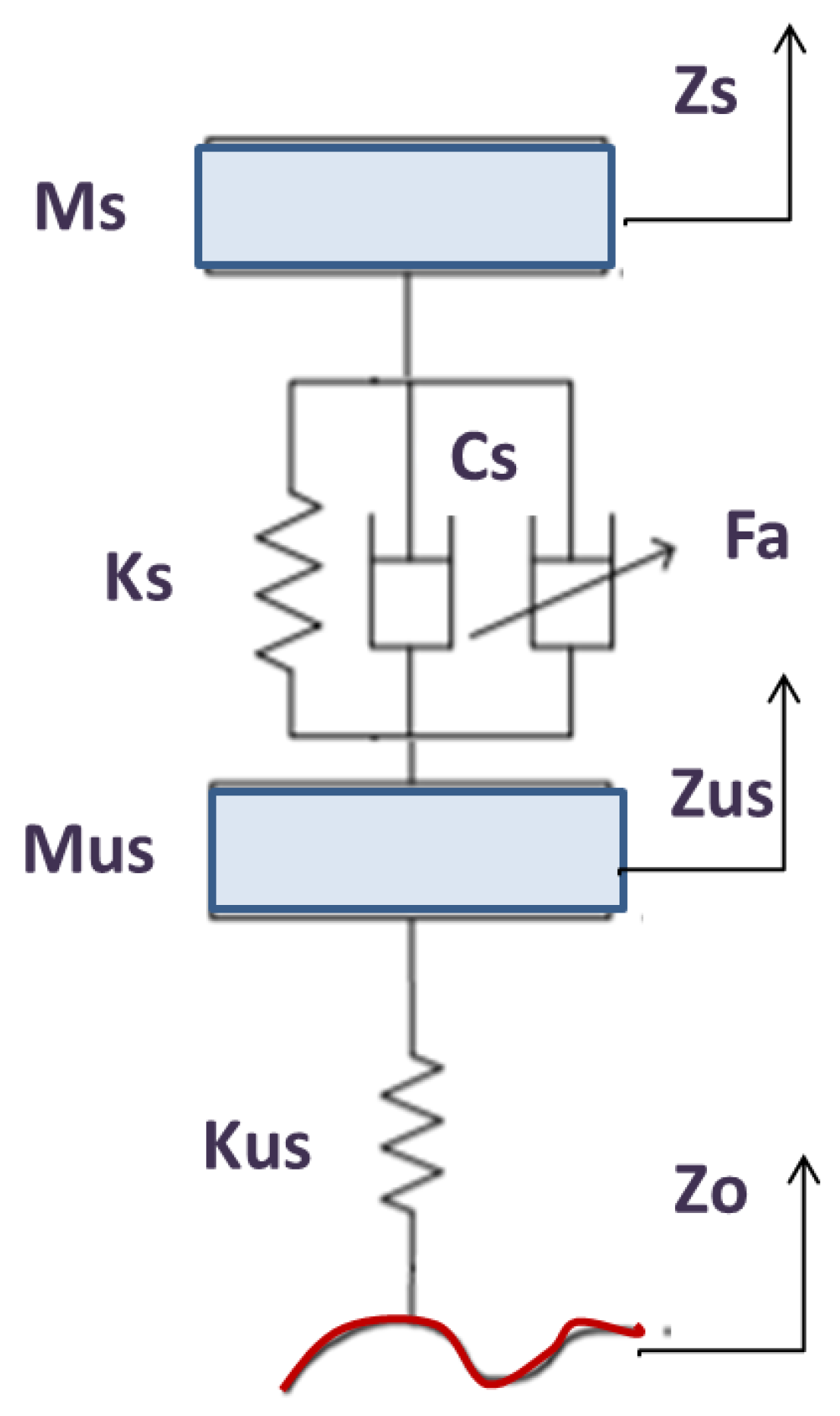
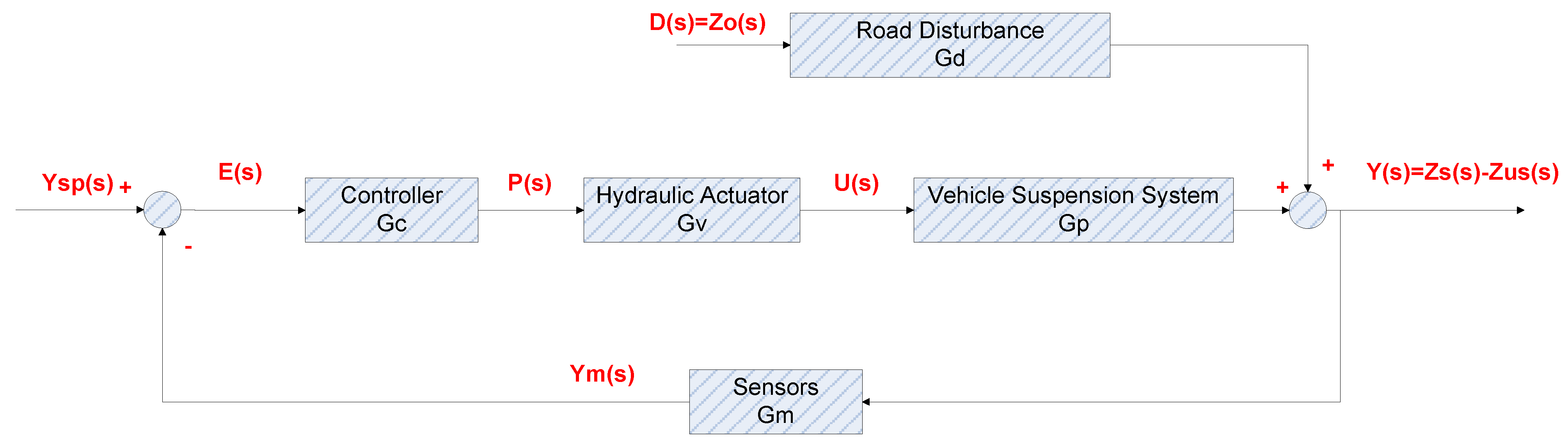
The core aim of the suspension system (see Figure 1) is to isolate the vehicle’s cabin from external road disturbances (e.g., it separates the car body from the wheels) in order to maximize the driving comfort for the passengers and ensure car stability. Another important role of the suspension system is to keep the wheel in contact with the road surface, as vibrations may be harmful to the passengers and the vehicle itself. These requirements for improved driving comfort and passenger safety have pushed car manufacturers to develop new active suspension systems. This type of suspension has the ability to adapt to harsh road surface conditions and is realized through the ability to store, dissipate and utilize energy within the system. Compared with the passive suspension (open loop without a control action), the active suspension performs better due to the force/power actuator. The actuator is a mechanical control system, which is mounted on the suspension, and can be pneumatic, hydraulic, electromagnetic, etc. The controller collects data from various sensors mounted on the vehicle that can analyze the road profile before any control action.

The design and simulation of a car suspension can be found in various forms in the literature. Most studies take a mathematical model for the active suspension into account and simulate it along with a (properly tuned) PID controller. In most case studies, simulations using a hydraulic actuator and tested in various road surface scenarios (uneven road, potholes and random road entrances) prove to be an established line of work. Such results have proven that the active suspension system with PID control improves driving comfort [6]. In [7], a significant effort was made to reduce the motion of a rail car body and the damper. Τhe PID controller was tuned through the Ziegler–Nichols methodology, and the simulated results between the passive and the active suspension system proved that the active suspension system with PID control improves ride comfort, gives a low peak overshoot (amplitude) and a faster settling time. Another group of studies discussed the performance of a PID controller (tuned with the Ziegler–Nichols method or with fuzzy methods) in a semi-active suspension of a vehicle. Again, the results proved that the active suspension system significantly improves driving comfort [8,9,10]. An interesting approach was reported in a study by A. Al-Zughaibi and H. Davies [11]. The controller was designed using the Routh–Hurwitz stability criterion and the respective simulations were carried out in a system with unknown time delays, different masses and road disturbance. The simulation results showed a significant improvement in performance and disturbance rejection. A quite interesting study using a combination of commercial software (used for extracting vehicle responses) and control design investigated the performance of a K-seat-based PID that is able to enhance motion comfort [12]. Along the same trend, J. Zhu et al. [13] worked on the nonlinear modeling and control of emergency rescue vehicles (e.g., active suspension systems in fire trucks) that lack body stability. Their disturbance rejection control design provided a complementary perspective to the results derived from feedback control implementation.

Moving on to modern control techniques, a neural-network-based model predictive controller (NN-MPC), designed for a non-linear servo-hydraulic vehicle suspension system, was compared to a PID controller. The analysis revealed the superior performance of the NN-MPC over the PID, as it showed a better tracking of the set-point, despite the disturbances that emerged [14]. J. Kim et al. [15] developed an MPC algorithm for semi-active suspension systems with road preview that managed to improve both the ride comfort and the road-handling performance. In particular, the damping force (input variable) was minimized towards achieving predefined trajectories. A detailed mathematical methodology based on multi-agent communication topology and MPC was presented by N. Zhang et al. [16] with an aim to minimize the vertical acceleration, pitch acceleration and roll acceleration of the vehicle body. Another meaningful case study dealt with the development of controllers in motors [17]. The control system was realized and tuned by an artificial intelligence strategy that is based on heuristic optimization techniques (particle swarm optimization, PSO). At first, the development of the mathematical model of the DC motor was carried out. Then, a feedback control system was applied under the adaptive PSO and the conventional Ziegler–Nichols method. The simulation and comparison of the above controller with the PSO and Ziegler–Nichols tuning methods showed that the PSO algorithm can be effectively used to tune the PID controller. 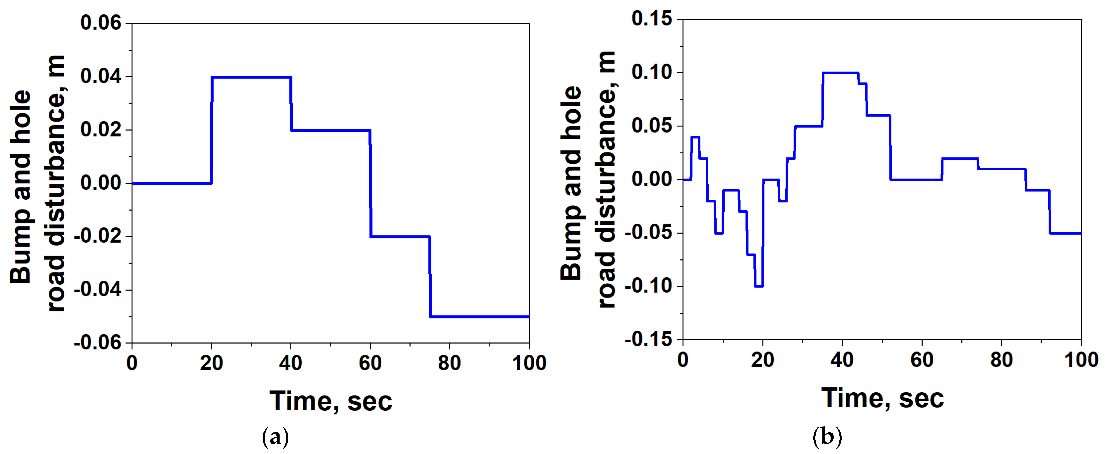In [18], three tuning methods were used for a PID controller, (heuristic tuning, Ziegler–Nichols tuning and the iterative learning algorithm). Afterwards, the simulation and comparison of the above-mentioned tuning methods, as well as of the comparison between the passive and active suspension system, were carried out for scenarios of three different road disturbances (bump and hole, sinusoidal and random input). The outcome of the study is that the active suspension system performs better than the passive suspension system, whereas the PID controller that was tuned by the iterative learning algorithm performed better than the other two tuning methods. In a more detailed study regarding the development of a full vehicle model, an adaptive PID control was designed [19]. Specifically, this study is worth mentioning because it developed an adaptive controller for active suspension systems with parameter uncertainties. Their aim was to improve the transient response of the body and to save the communication resources of the in-vehicle network. An interesting study that tried to address problems relating to gain estimation was presented by Y. Jeong et al. [20]. This group designed a linear-quadratic (LQ) static output feedback with a 2-DOF quarter-car model for an active suspension system. This type of control uses available sensor signals measured in real vehicles and formulates an optimization problem that can be solved via a heuristic optimization method. It was concluded that the proposed controller showed the best performance in terms of ride comfort.

Several other studies can also be found in the literature and include control approaches such as the linear quadratic regulator [21,22,23], adaptive sliding control [24], H∞ control [25,26], advanced fuzzy control [27,28], optimal control [15,29] and neural-network-based methods for tuning [30,31].

Aside from vehicles, specifically those in train suspension systems, the study by X. He et al. in [32] studied the riding comfort of high-speed trains (which affect the travel experience of passengers) and aimed at reducing the vibrations through the application of a vertical dynamics model of railway vehicles. Furthermore, a unique study with actual implementation scenarios was reported by K. Ikeda et al. [33]. The purpose of this study was to estimate the psychological state of an occupant based on biometric information. Based on the research findings, the ride quality of occupants while driving can be recorded and control algorithms can be retrofitted in real time.

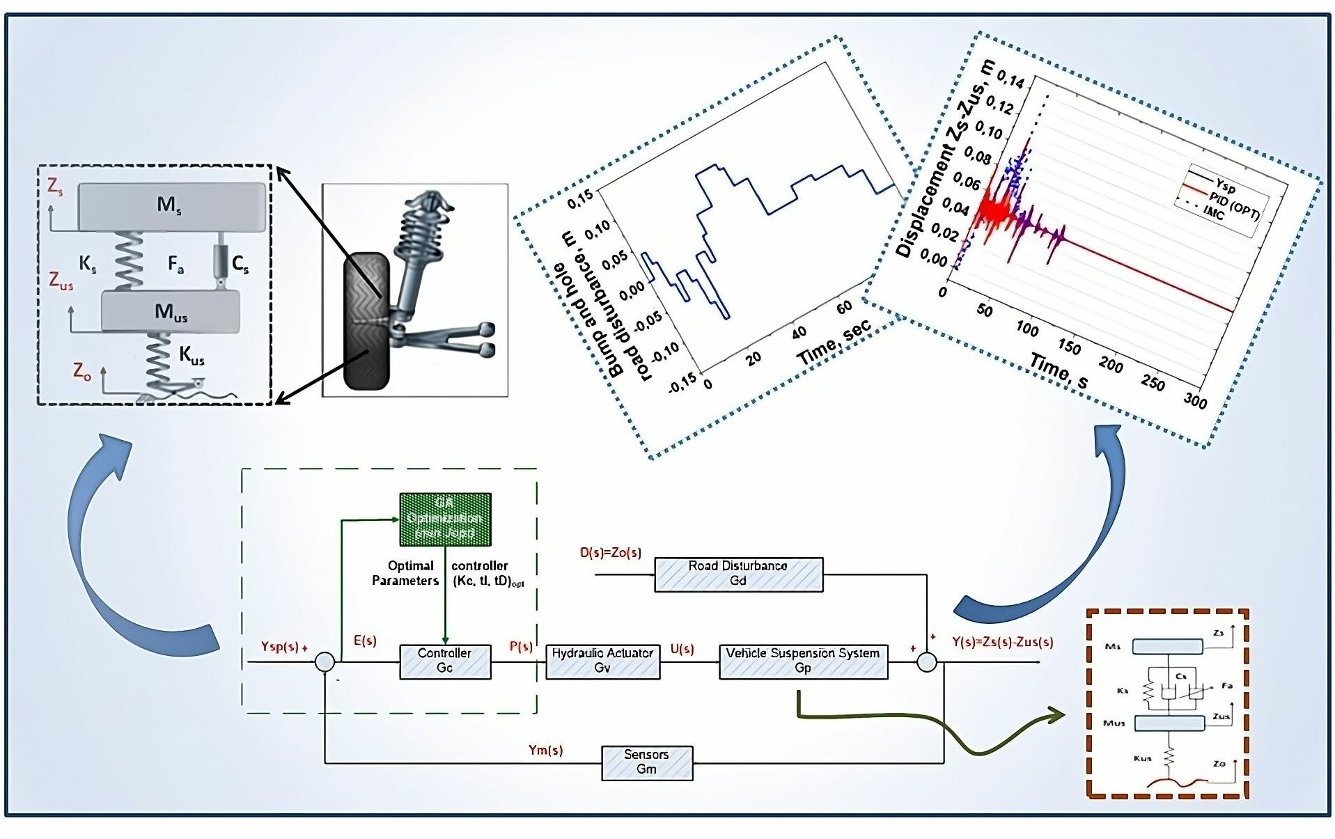
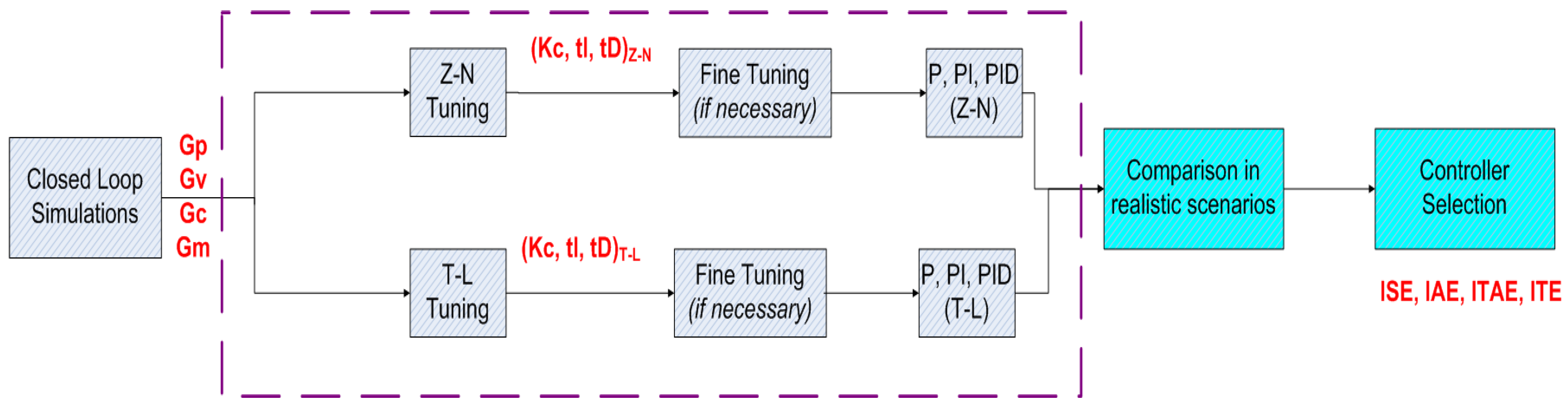
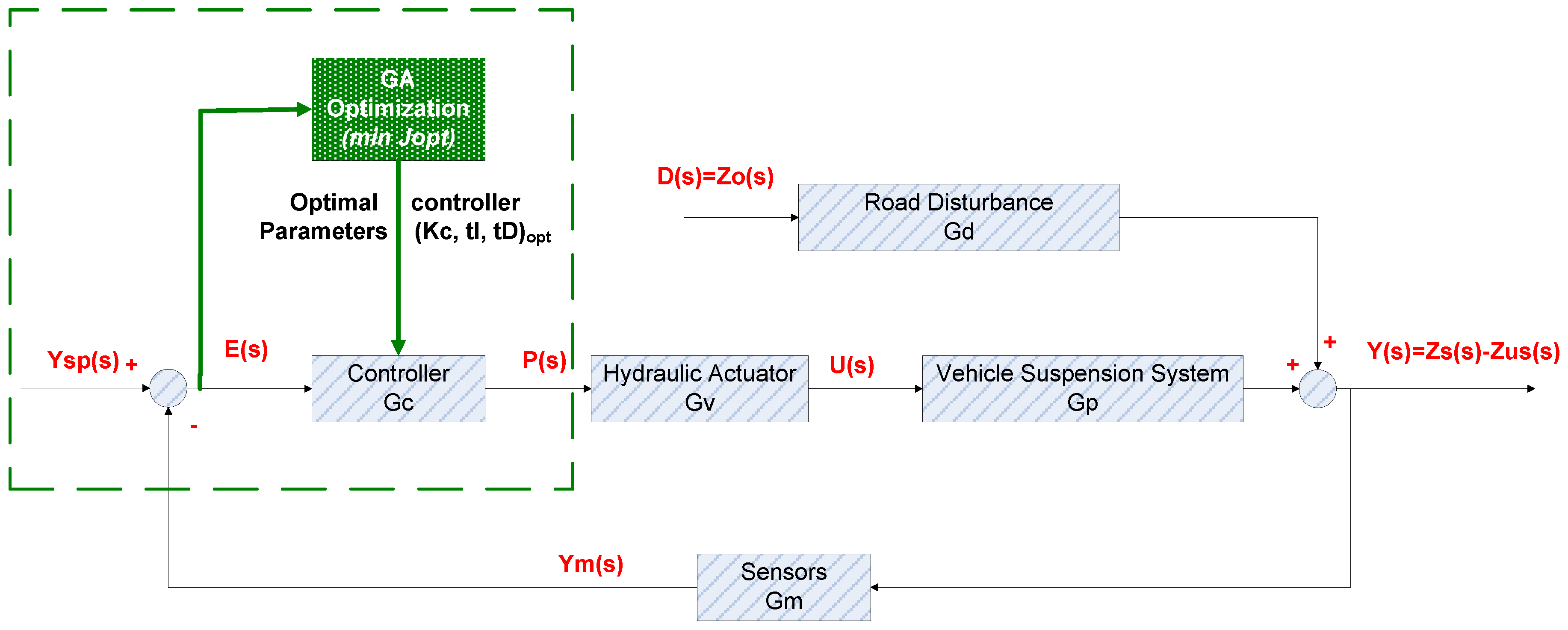
Since several studies dealing with vehicle suspensions have been carried out in the literature, the focus of this study is not claimed to be unique among such interesting and useful studies. The vision of the present study is to provide a simplified step-by-step approach that can be used as an applied example of modeling and control for engineering students’ lectures. The concept of active suspension systems has significant benefits, as it can be comprehensively taught via the following consecutive educational requirements: (a) the set-up of the mathematical model of a quarter of a car (¼) active suspension in the dual form of differential equations, state-space model and transfer functions, (b) the design and application of a feedback control system based on P, PI and PID controllers, (c) the design and application of a feedback control system based on internal model control (IMC) and (d) the evaluation of the controllers’ performance under different road conditions (including disturbances). The above are accompanied by applied tuning techniques such as the methodologies of Ziegler–Nichols and Tyreus–Luyben and optimal tuning through genetic algorithms (GA).

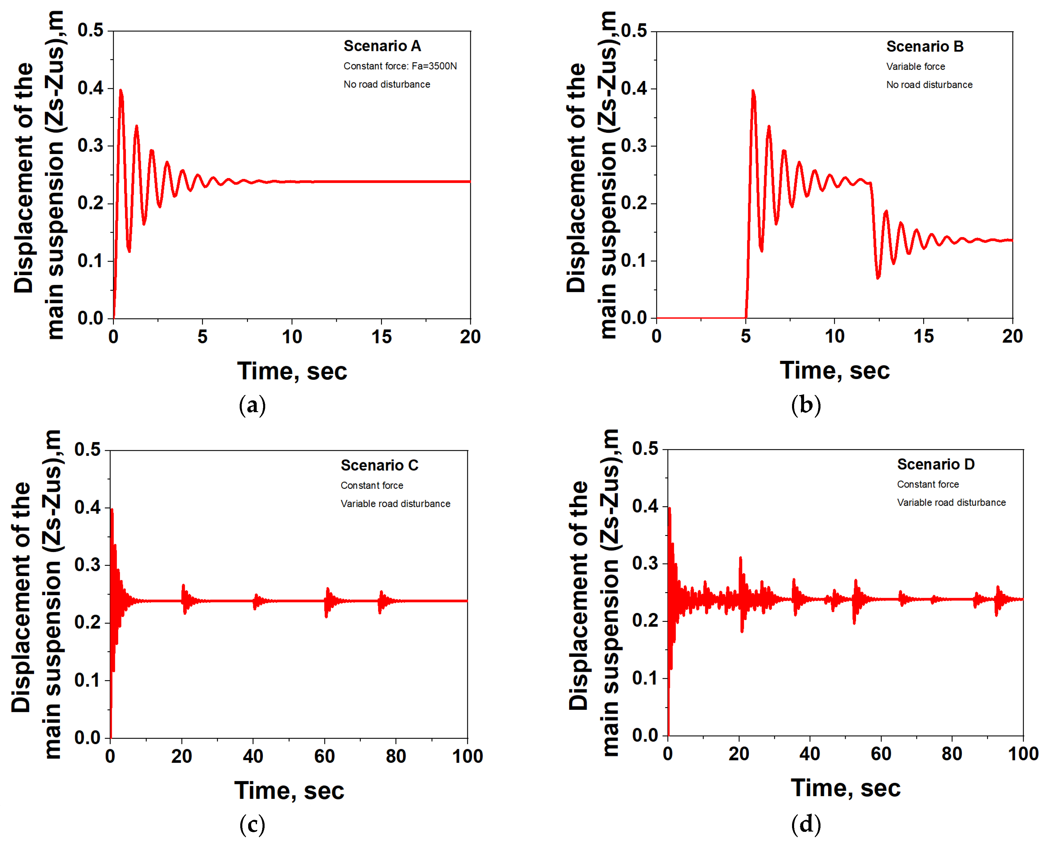
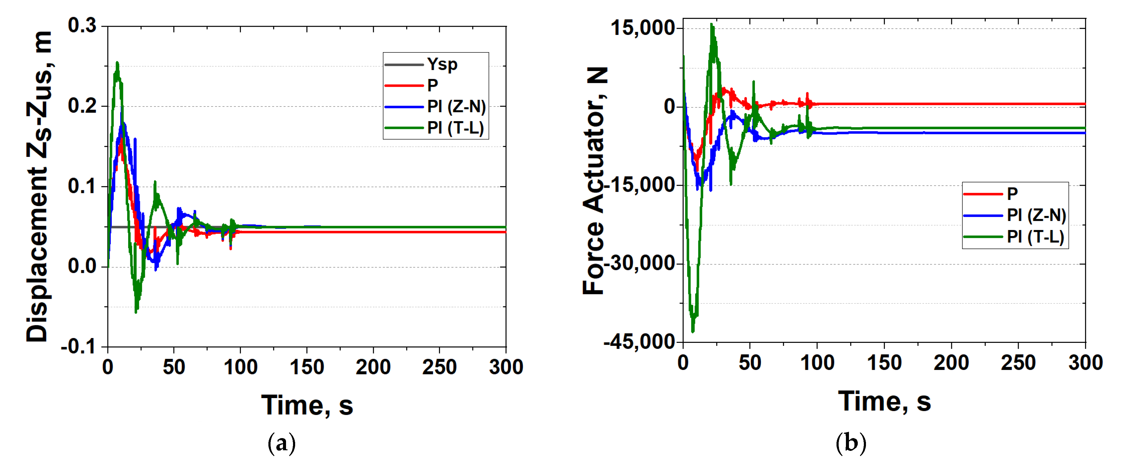
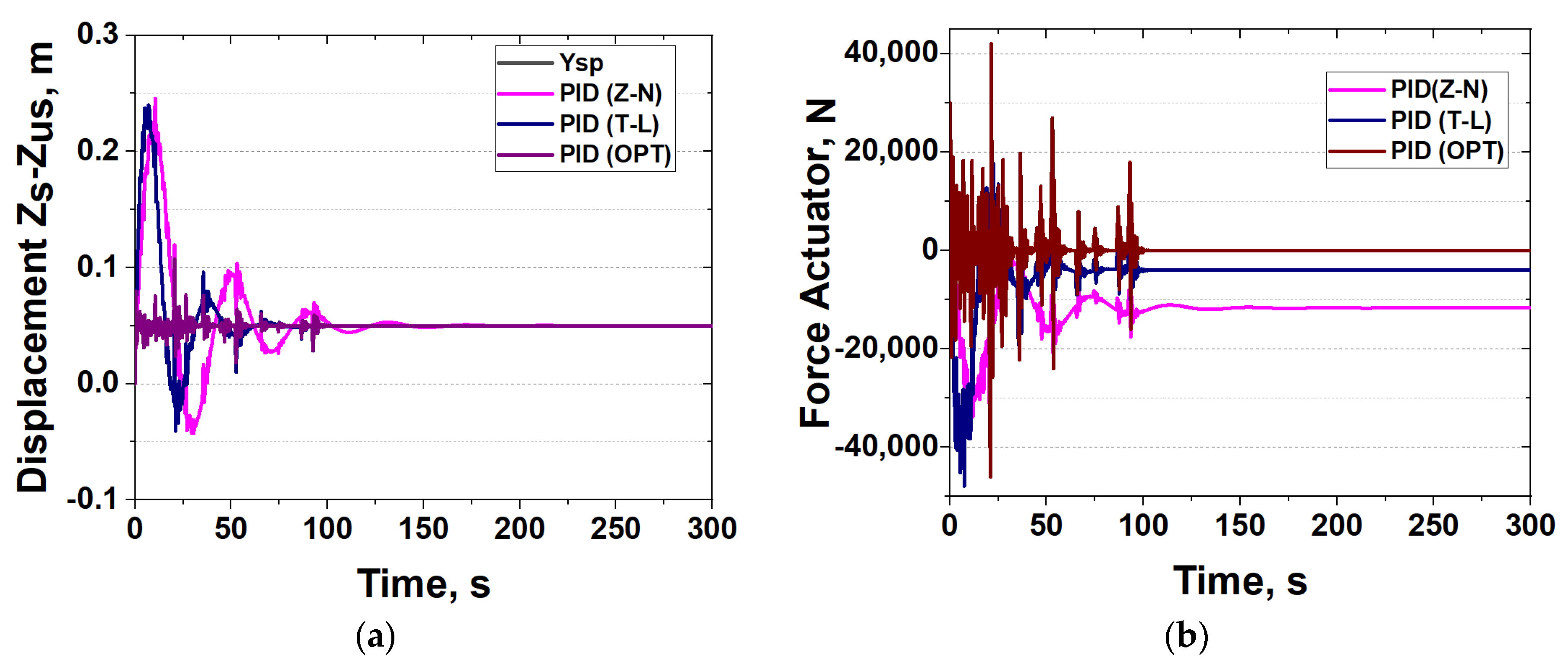
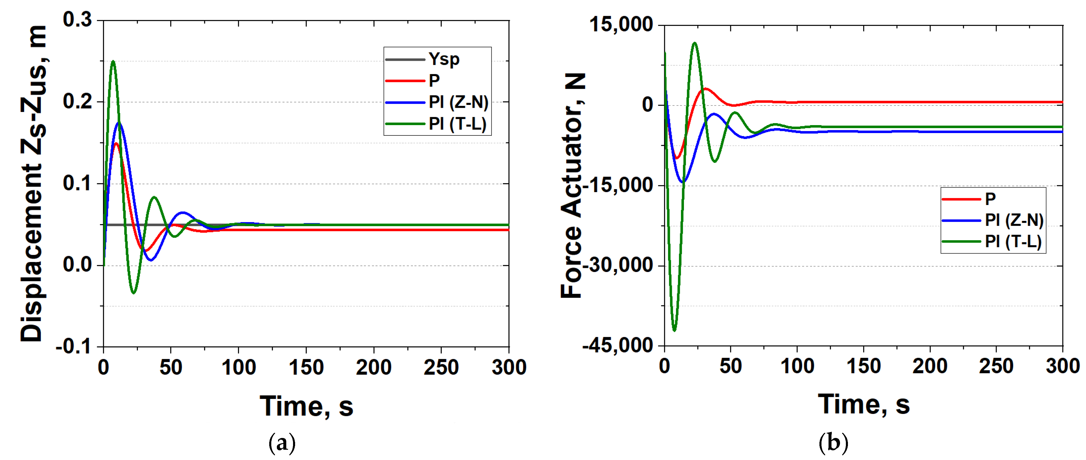
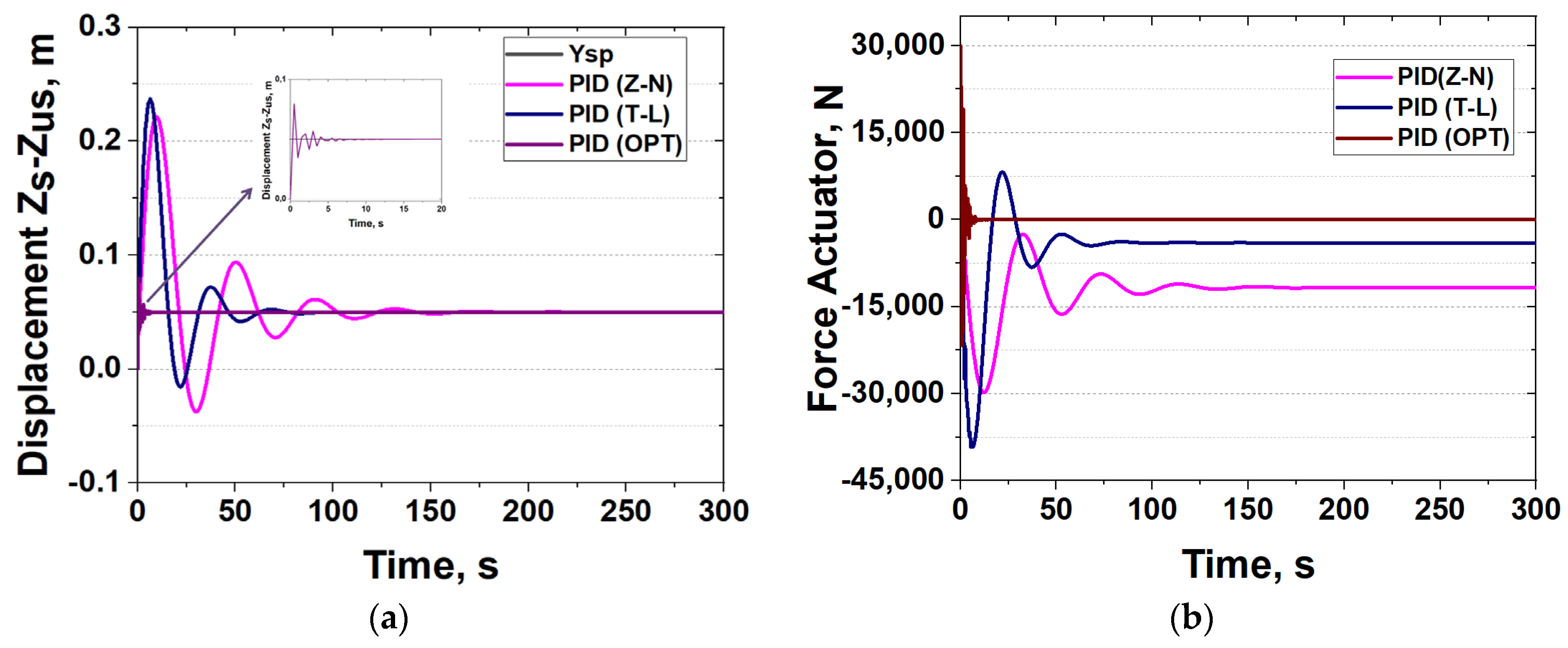
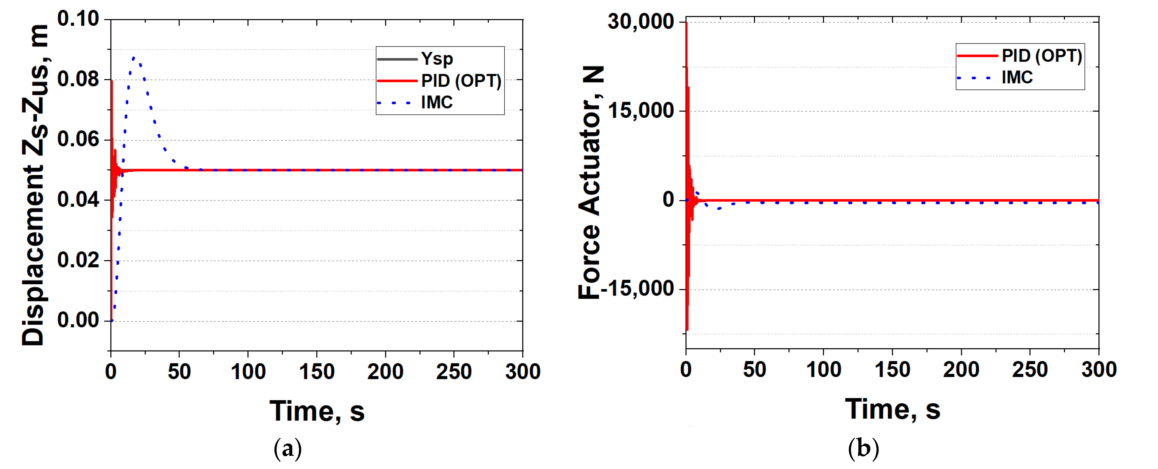
The structure of the paper is as follows: Section 2 presents the mathematical model of the active suspension system. In this section, open loop simulations are used to evaluate the system dynamics under scenarios of varying input force and by applying random disturbances. Next, Section 3 designs the feedback control system that is realized in the form of P, PI and PID controllers (tuned via the Ziegler–Nichols and Tyreus–Luyben methodologies), in the form of an optimal PID controller tuned via a GA optimization framework and in the form of a feedback internal model controller. The comparison of the performance of all controllers is evaluated (Section 4) in different scenarios that include set-point variations with or without the presence of road disturbances.

2. Mathematical Model of the Active Suspension System

2.1. 2nd and 1st (Reduced) Order Differential Equations

Figure 2 shows a typical active suspension system that consists of a passive spring, a passive damper and an actuator. The actuator can be hydraulic, pneumatic or electromagnetic. Through this element, the controller can decide whether to add or dissipate energy with the help of measurements (sensors that could provide road profile data). When the mechanical spring, damper and actuator are connected, a hydraulic actuator can be used and is able to control both the mass of the tire (M_us) and the vehicle mass or vehicle body (M_s).

The equations of motion can be written as follows (In the case of F_a = 0, the system reduces to the open loop passive suspension with no control actions):

$$M_s\frac{d^2{Z}_s}{d{t}^2}=F_a(t)-K_s(Z_s(t)-Z_{us}(t))-C_s(\frac{d{Z}_s}{dt}-\frac{d{Z}_{us}}{dt})$$

(1)

$$M_{us}\frac{d^2{Z}_{us}}{d{t}^2}=-F_a(t)+K_{us}(Z_o(t)-Z_{us}(t))+K_s(Z_s(t)-Z_{us}(t))+C_s(\frac{d{Z}_s}{dt}-\frac{d{Z}_{us}}{dt})$$

(2)

where F_a [N] is the control force from the hydraulic actuator, M_s [kg] is the sprung mass, M_us [kg] is the unsprung mass, Z_s [m] is the sprung mass position, Z_us [m] is the unsprung mass position, Z_o [m] is the road surface anomaly, K_s [N/m] is the suspension spring (stiffness), K_us [N/m] is the tire spring element and C_s [N·s/m] is the damping co-efficient of the variable shock absorber.

Due to the fact that Equations (1) and (2) are second-order differential equations, auxiliary variables (x₁, x₂, x₃, x₄) can be used, so that the reduction process to differential equations of a first-order magnitude can be carried out. Based on the above, there are four (4) state variables (x₁, x₂, x₃, x₄) and one (1) output is defined as y = (x₁ − x₃) = (Z_s − Z_us):

$$\begin{array}{ccc}{x}_1=Z_s\hfill & \Rightarrow \hfill & \frac{d{x}_1}{dt}=x_2\hfill \\ x_2=\frac{d{Z}_s}{dt}\hfill & & \frac{d{x}_2}{dt}=\left(\frac{F_a}{M_s}\right)-\left(\frac{K_s}{M_s}\right)·x_1+\left(\frac{K_s}{M_s}\right)·x_3-\left(\frac{C_s}{M_s}\right)·x_2+\left(\frac{C_s}{M_s}\right)·x_4\hfill \\ x_3=Z_{us}\hfill & & \frac{d{x}_3}{dt}=x_4\hfill \\ x_4=\frac{d{Z}_{us}}{dt}\hfill & & \frac{d{x}_4}{dt}=-\left(\frac{F_a}{M_{us}}\right)+\left(\frac{K_{us}}{M_{us}}\right)·Z_0-\left(\frac{K_{us}}{M_{us}}\right)·x_3+\left(\frac{K_s}{M_{us}}\right)·x_1-\left(\frac{K_s}{M_{us}}\right)·x_3+\left(\frac{C_s}{M_{us}}\right)·x_2-\left(\frac{C_s}{M_{us}}\right)·x_4\hfill \\ & \Rightarrow \hfill \\ & & y=(x_1-x_3)\hfill \end{array}$$

(3)

2.2. State-Space form Equations

From the above set of four (4) differential equations, the desired state-space form can be formulated and used thereafter in the following form {x(t₀) = x₀ = 0}:

$$\begin{array}{l}\stackrel{·}{x}(t)=A·x(t)+B·u(t)+E·d(t)\\ y(t)=C·x(t)+D·u(t)\end{array}$$

(4)

The state-space model of matrices A, B, C, D, E can be realized:

$$\left[\begin{array}{l} \frac{d{x}_1}{dt}\\ \frac{d{x}_2}{dt}\\ \frac{d{x}_3}{dt}\\ \frac{d{x}_4}{dt}\end{array}\right]=\left[\begin{array}{cccc}\hfill 0\hfill & \hfill 1\hfill & \hfill 0\hfill & \hfill 0\hfill \\ \hfill -\frac{K_s}{M_s}\hfill & \hfill -\frac{C_s}{M_s}\hfill & \hfill \frac{K_s}{M_s}\hfill & \hfill \frac{C_s}{M_s}\hfill \\ \hfill 0\hfill & \hfill 0\hfill & \hfill 0\hfill & \hfill 1\hfill \\ \hfill \frac{K_s}{M_{us}}\hfill & \hfill \frac{C_s}{M_{us}}\hfill & \hfill -\frac{(K_s+K_{us})}{M_{us}}\hfill & \hfill -\frac{C_s}{M_{us}}\hfill \end{array}\right]·\left[\begin{array}{l}{x}_1\\ x_2\\ x_3\\ x_4\end{array}\right]+\left[\begin{array}{l}0\\ \frac{1}{M_s}\\ 0\\ -\frac{1}{M_{us}}\end{array}\right]·F_a+\left[\begin{array}{l}0\\ 0\\ 0\\ \frac{K_{us}}{M_{us}}\end{array}\right]·Z_o$$

(5a)

$$y=\left[1 0 -1 0\right]·\left[\begin{array}{l}{x}_1\\ x_2\\ x_3\\ x_4\end{array}\right]+[0]·F_a$$

(5b)

2.3. Mathematical Model in the Form of Transfer Functions

Based on the above, the transfer functions of the process (G_p) and of the disturbance (G_d) can be derived from the following relationships:

$$\begin{array}{l}{G}_p(s)=\frac{Y(s)}{U(s)}=\frac{Z_s(s)-Z_{us}(s)}{F_a(s)}=C·{(sI-A)}^{-1}·B+D\\ G_p(s)=\frac{(M_{us}+M_s)·s^2+K_{us}}{(M_s·s^2+C_s·s+K_s)·(M_{us}·s^2+C_s·s+K_s+K_{us})-{(C_s·s+Ks)}^2}\end{array}$$

(6a)

$$\begin{array}{l}{G}_d(s)=\frac{Y(s)}{D(s)}=\frac{Z_s(s)-Z_{us}(s)}{Z_o(s)}=C·{(sI-A)}^{-1}·E\\ G_d(s)=\frac{-K_{us}·M_s·s^2}{(M_s·s^2+C_s·s+K_s)·(M_{us}·s^2+C_s·s+K_s+K_{us})-{(C_s·s+Ks)}^2}\end{array}$$

(6b)

$$Y(s)=G_p(s)·U(s)+G_d(s)·D(s)$$

(6c)

Before proceeding to the series of open loop simulations, the main parameters of the active suspension need to be defined and are shown in

Table 1. Active suspension system parameters.

System Parameters	Values	Units
Ms	243	kg
Mus	40	kg
Cs	370	N∙s/m
Ks	14,671	N/m
Kus	124,660	N∙s/m
Initial Conditions	0 at t = 0 s

.

2.4. Open Loop Simulations

Open loop simulations show the dynamic performance of the suspension system when no control action is applied. Such simulations highlight the need for a proper control design since oscillations, high overshoots and prolonged settling times are always reported. Certainly, closed loop simulations are more important, but for a simplified approach that is trying to force engineering students to delve into control systems, it is worth devoting a few lines to the open loop performance of the suspension system.

Based on the mathematical model of Section 2 (in either form of the differential equations, state-space and Laplace domain), we performed the following simulation scenarios regarding road disturbances (see also Figure 3a,b regarding scenarios C and D):

• (A) Constant force of F_a = 3500 N with no road disturbance Z_o = 0 m.
• (B) Variable force with no road disturbance Z_o = 0 m:

$$\begin{array}{l}{F}_a=\{0 \mathrm{N}, \hspace{1em} \mathrm{for} 0<t<5 \mathrm{s}\}\\ F_a=\{3500 \mathrm{N}, \mathrm{for} 5\le t\le 12 \mathrm{s}\}\\ F_a=\{2000 \mathrm{N}, \mathrm{for} t>12 \mathrm{s}\}\end{array}$$

• (C) Constant force of F_a = 3500 N and variable (short time bump and hole) road disturbance:

$$\begin{array}{l}{Z}_o=\{0 \mathrm{m},\hspace{1em}\hspace{1em}\mathrm{for} 0<t<20 \mathrm{s}\}\\ Z_o=\{0.04 \mathrm{m},\hspace{1em}\mathrm{for} 20\le t\le 40 \mathrm{s}\}\\ Z_o=\{0.02 \mathrm{m},\hspace{1em}\mathrm{for} 40<t<60 \mathrm{s}\}\\ Z_o=\{-0.02 \mathrm{m}, \mathrm{for} 60\le t\le 75 \mathrm{s}\}\\ Z_o=\{-0.05 \mathrm{m}, \mathrm{for} t>75 \mathrm{s}\}\end{array}$$

• (D) Constant force of F_a = 3500 N and random (continuous bump and hole) road disturbance: Z_o = {random variation for 0 < t < 100 s}

Figure 3. Bump and hole road disturbance (road anomaly) (a) short-term and (b) long-term.

Figure 3. Bump and hole road disturbance (road anomaly) (a) short-term and (b) long-term.

Figure 4a–d show the displacement deviation (with the output variable of our model as y = x₁ − x₃ = Z_s − Z_us) under the four (4) different and arbitrarily selected scenarios A to D. As can be seen in Figure 4a, by applying a constant force equal to 3500 N, the suspension system oscillates for a short period of nearly 8–10 s and stabilizes at a new operation point (0.24 m displacement with a peak overshoot of 0.4 m). Similarly, Figure 4b shows the effect of applying a variable force of 0, 2000 and 3500 N. Initially, the system is at the desired peaceful state (no oscillations). At t = 5 s, a 3500 N force is applied for a short period of time (until the 12th second) and then a sudden force reduction at 2000 N is applied. In scenario B, the steady-state displacement is reduced from 0.24 m to 0.135 m, with descending and detrimental (for the vehicle and the passengers) oscillations. Proceeding to scenario C and D in Figure 4c,d, the effects of short- and long-term bump and hole disturbances (under a constant force of 3500 N) are observed, respectively. During the effect of the disturbance, the suspension system oscillates (the higher the disturbance → the higher the oscillation magnitude) and stabilizes at the displacement of 0.24 m in both scenarios. Clearly, scenario D is a worst-case scenario, where it is seen that inside the vehicle, the passengers suffer significantly from road anomalies.

3. Feedback Control System Design

The open loop simulation scenarios presented above show that a control system is needed if we want to provide ride comfort for the vehicle passengers. Its aim should be quick disturbance rejection (e.g., from road anomalies) in a way that will not stress the hydraulic actuator of the feedback controller. With this in mind, this section is devoted to the investigation of the suitability of two types of controllers, (a) conventional P, PI and PID controllers and (b) internal model control, IMC. Figure 5 shows the proposed feedback control system. The transfer functions of each element involved, are shown afterwards in

Table 2. Closed loop transfer functions (based on Table 1).

Transfer Function
Gp(s)	$\frac{283·s^2+124660}{(243·s^2+370·s+14671)·(40·s^2+370·s+139331)-{(370·s+14671)}^2}$
Gd(s)	$\frac{-30292380·s^2}{(243·s^2+370·s+14671)·(40·s^2+370·s+139331)-{(370·s+14671)}^2}$
Gv(s)	$\frac{1}{10s+1}$
Gm(s)	$\frac{1}{30s+1}$
Gc(s)	Equations (7) and (10)

.

3.1. PID Controller

The PID controller takes the following form:

$$\mathrm{PID}\mathrm{Controller:} G_c(s)=K_c·(1+\frac{1}{\tau I·s}+\tau D·s)$$

(7)

In order to apply and evaluate a feedback control system, the following steps are implemented and discussed in detail afterwards (see also Figure 6 and Figure 7 for the GA framework):

• Step 1: Tuning of the different (P, PI and PID) controllers via the Ziegler–Nichols and Tyreus–Luyben methods and a by using genetic algorithms (PID (OPT)).
• Step 2: Implementation of the selected type of controllers (either, P, PI or PID) and fine tuning (only if necessary for the cases using Ziegler–Nichols and Tyreus–Luyben tuning) and verification via realistic simulation scenarios.
• Step 3: Selection of the best type of controller to be compared with the IMC afterwards.

Figure 6. Conventional tuning methodology for PID controllers.

Figure 6. Conventional tuning methodology for PID controllers.

Figure 7. Optimal tuning methodology for PID controllers.

Figure 7. Optimal tuning methodology for PID controllers.

The methodologies of Ziegler–Nichols and Tyreus–Luyben tuning have some limitations in terms of applications. Some of these refer to (a) the tuned parameters of a PID are not optimal and require fine tuning prior to implementation, (b) the output of the controller has its own limitations (e.g., a maximum force to be applied) and these limits cannot be surpassed due to mechanical reasons and (c) PID control might end up with saturation issues that can only be solved through anti-wind-up techniques (it is beyond the scope of this study to include their implementation).

3.2. Optimal Tuning Via Genetic Algorithms

The evaluation of optimal PID controllers is also an interesting topic of research in the literature. M. Kaldas et al. [34] estimated controller parameters by using a gradient-based optimization routine with an objective function that includes both ride comfort and road holding. The ride performance of the road preview control strategy was evaluated through a stochastic road profile and the results highlighted the importance of the road preview control strategy, which significantly improves ride performance. A similar approach was recently published by G. Abbas et al. [35], who used a similar optimization pattern with the integral squared error (ISE) as their objective function. In that particular study, a low overshoot and fast settling times have been reported.

In this study, we selected the MATLAB optimization toolbox for the optimal PID tuning [36]. Specifically, we selected the genetic algorithm (GA) to be our optimization solver since it is an established method for both constrained and unconstrained problems. The algorithm modifies a population of individual solutions. For each step, the GA randomly selects individuals from the current population and uses them as parents to produce the children for the next generation. Over successive generations, the population evolves and the best point in the population approaches an optimal solution [36]. For our problem, the optimal tuning was performed by seeking the optimal solution (equivalently the pairing of the PID controller parameters Kc, τΙ and τD) that minimizes the performance criterion of the squared error:

$$J_{opt}=\min [{\displaystyle \underset{0}{\overset{t}{\int }}{(Y(t)-Y_{sp}(t))}^2}dt]$$

(8)

where Y_sp(t) is the set-point in m and Y(t) is the Z_s(t) − Z_us(t) system output variable in m.

Table 3. Selection of controllers based on the Ziegler-Nichols (Ζ-Ν), Tyreus-Luyben (T-L) and optimal (OPT) tuning method.

Controller	Kc	τI	τD
P (Z-N)	98,500	-	-
PI (Z-N)	88,650	23.79	-
PID (Z-N)	118,200	14.27	0.357
PI (T-L)	197,000	62.8	-
PID (T-L)	197,000	62.8	0.453
PID (OPT)	19,461	40	7.39

shows the controller parameters (Kc gain, τI integral time and τD derivative time) for steps 1 and 2. In the cases of Ziegler–Nichols and Tyreus–Luyben tuning, it was observed that all controllers led to a very aggressive control action and we had to reduce Kc by a factor of 100 and increase τI by a factor of 10 (as respective to the critical gain and period that were found through root locus analysis at the values of Kcr = 1.9 × 10⁷ and Pcr = 2.85 s). The implementation and comparison of the above controllers will be compared and discussed in Section 4.

3.3. IMC Controller

The IMC controller can be easily designed based on the system’s Gp function (see Table 2) via the following equation [37]:

$$G_P(s)={G^{-}}_p(s)·{G^{+}}_p(s)$$

(9)

where ${G^{-}}_p\left(s\right)$ is the minimum phase and ${G^{+}}_p\left(s\right)$ is the non-minimum phase (which will be equal to 1 in our case). In our case that we have the transfer functions of G_c and G_m, the theory allows as to add them (unless it is mentioned otherwise).

The Gc(s) transfer function of the controller can be derived through the following equation:

$$G_c(s)=\frac{1}{{G^{-}}_p(s)}·\frac{1}{{(\lambda ·s+1)}^r-{G^{+}}_p(s)}$$

(10)

where r is the difference between the order of the denominator and the order of the nominator and λ is a time constant that can be defined from the user (we will use λ = 5 in our case).

3.4. Controller Performance Criteria

In order to evaluate and screen the performance of the controllers, a series of controller performance criteria have been used [37,38]:

Integral Squared Error (ISE)	Integral time Squared Error (ITSE)
$ISE={\displaystyle \underset{0}{\overset{\infty }{\int }}{e}^2(t)dt}$	$ITSE={\displaystyle \underset{0}{\overset{\infty }{\int }}t·e^2(t) dt}$
Integral Absolute Error (IAE)	Integral Time Absolute Error (ITAE)
$IAE={\displaystyle \underset{0}{\overset{\infty }{\int }}\left|e(t) \right| dt}$	$IATE={\displaystyle \underset{0}{\overset{\infty }{\int }}t·\left|e(t) \right| dt}$

4. Evaluation and Comparison of Feedback Controllers

Based on the analysis performed in the previous section, the evaluation of all feedback controllers is to be compared under two road scenarios:

(a)

Scenario 1: the displacement Z_s − Z_us is 0.05 m (set-point) and no disturbances are applied.

(b)

Scenario 2: the displacement Z_s − Z_us is 0.05 m (set-point) and disturbances are applied as shown in Figure 3b (with the difference that the time period will be prolonged to 300 s).

4.1. Simulation Scenario 1: Set-Point Tracking under No Disturbances

Based on the above two scenarios, the P, PI and PID controllers that were tuned via Z-N and T-L methods, and presented in Table 3, are compared in the following figures. The force actuator represents the exit variable from the hydraulic actuator, U(s), shown in Figure 5.

Table 4. Performance criteria for the comparison of controllers during simulation scenario 1.

	Overshoot, %	Peak Time, s	Rise Time, s	Settling Time (±5%), s	Steady-State Error, m
P	198.6	9	1.8	--	0.0062
PI (Z-N)	245.6	10	1.9	90.5	0
PI (T-L)	400	4	0.8	82.5	0
PID (Z-N)	340.4	9	1.3	118.5	0
PID (T-L)	370	6	0.3	59.5	0
PID (OPT)	59	0.5	0.3	4.5	0
IMC	74	16.5	8.5	46	0

summarizes control parameters such as overshoot (%), peak time, rise time, settling time and steady-state error for Scenario 1 (the IMC will be discussed in Section 4.3).

As shown in Figure 8a, the P controller (red color) fails to reach the set-point of 0.05 m and after 90–100 s reaches its steady state value at 0.0435 (featuring a persistent steady-state error of 13%). On the other hand, both PI controllers reach the desired set-point at nearly the same settling point of ~80–90 s after a few oscillations. The PI controller tuned via the T-L method shows a more aggressive action since an overshoot of 0.2 m (~400%) occurs, whereas the PI controller tuned via the Z-N method shows a lower, but still high, overshoot of 0.1 m (~245%). Figure 8b shows the respective dynamic performance of the control actuator for the three (3) controllers. As expected, PI tuned via the T-L method shows the most aggressive action, and the P controller the least aggressive.

Following the above analysis, Figure 9a shows the performance of the three (3) PID controllers. As can be seen, the optimal PID controller shows an extremely superior performance since the values of overshoot (59%) and settling time (<5 s) are extremely low. On the other hand, the two PID controllers (Z-N and T-L) present a descending oscillation that is more evident in the PID (Z-N) with a settling time of ~120 s as compared to the lower settling time of the PID (T-L) at ~60 s. Meanwhile, both these controllers indicate a significant overshoot of 0.17–0.18 m (~340–370%). Figure 9b supplements the analysis by depicting the control actuator dynamics for the three PID controllers. As expected, the least action is provided by the optimal PID and the highest by the PID (Z-N) and the PID (T-L).

4.2. Simulation Scenario 2: Set-Point Tracking and Disturbance Rejection

Following the previous analysis, this subsection presents the control simulation of scenario 2. Since we have both a constant set-point tracking and a simultaneous disturbance rejection, we skipped the information regarding overshoot, peak time, rise time, etc., that are more or less similar to scenario 1 and shown in Table 4. As can be seen in Figure 10a, the P controller fails to reach set-point at 0.05 m, and after the effect of disturbances (see Figure 3b for the road anomaly profiles) it reaches its steady state value at 0.0435 (featuring a constant error of 13%). On the other hand, the other two PI controllers reach the desired set-point at nearly the same settling point after oscillating significantly during the disturbance emergence. The PI (T-L) controller shows more aggressive action in all time periods where a bump or hole is encountered, followed by a slightly more comfortable performance by the PI (Z-N). Figure 10b shows the respective dynamic performances of the control actuator for the three (3) controllers and, as expected, the PI (T-L) shows the most aggressive action and the P controller the least aggressive. Overall, the controller performances are similar to the ones in scenario 1, and the spikes refer to the emerged road anomalies.

Figure 11a shows the performance of the three (3) PID controllers. Similar to the previous case in scenario 1, the optimal PID controller shows an extremely superior performance as it exhibits the lowest oscillations (in magnitude and duration) among the three controllers. The two PID controllers (Z-N and T-L) present a more aggressive oscillation which is persistent over time. Among the two, the PID (T-L) shows a better performance in terms of low peaks and settling times. Figure 11b depicts the control actuator dynamics for the three PID controllers. As expected, the least overall action is provided by the optimal PID and the highest by the PID (Z-N). It is worth mentioning that the optimal PID presents a very aggressive action during the imminent disturbance effect, and this needs to be taken into account during implementation.

4.3. Simulation Scenarios 1 and 2: Comparison of IMC and Optimal PID Controllers

Based on the previous analyses in Section 4.1 and Section 4.2, it was revealed that the optimal PID is the best choice among all controllers. Hence, in this section, the IMC controller and the optimal PID will be compared in the same scenario 1 and in a modified scenario 2 (here, the disturbance shown in Figure 3b will be applied, not from t = 0, but from t = 100 s and thereafter). Regarding scenario 1, as shown in Figure 12a and Table 4, the optimal PID controller presents the lowest overshoot (59%) and settling time (4.5 s). The IMC presents an overshoot of 74% (see also Table 4) that last for about 45–50 s (settling time), but in a very smooth way. If we compare the control actions of both controllers in Figure 12b, we observe the minimum effort provided by the IMC (nearly zero action). This result shows that the actuator in the IMC controller design will face the least pressure during road riding and this is considered an asset of this feedback controller.

Regarding the modified scenario 2 shown in Figure 13a, the optimal PID controller presents the lowest overshoot and settling time during the disturbance emergence at t = 100 s and afterwards. The IMC indicates a very smooth performance in the same time period. If we compare the control actions of both controllers in Figure 13b, we can again observe the minimum effort provided by the IMC (nearly zero action). This result shows that the actuator in the IMC controller design will face the least pressure during road riding compared to the optimal PID. Clearly, this should be a concern during implementation, since min/max hard constraints on the actuator could lead to a problematic control action.

4.4. Performance Criteria and Critical Analysis

Table 5. Performance control criteria for scenario 1.

Performance Criterion	P	PI (Z-N)	PI (T-L)	PID (Z-N)	PID (Z-N)	PID (OPT)	IMC
ISE	0.239	0.406	0.716	0.780	0.592	0.004	0.065
IAE	6.721	5.692	6.532	8.911	5.550	0.138	2.126
ITSE	6.355	6.116	7.591	13.551	5.386	0.0012	0.916
ITAE	622.37	139.4	121.13	276.1	87.97	0.618	38.39

and

Table 6. Performance control criteria for scenario 2.

Performance Criterion	P	PI (Z-N)	PI (T-L)	PID (Z-N)	PID (Z-N)	PID (OPT)	IMC
ISE	0.247	0.413	0.720	0.787	0.597	0.0167	0.079
IAE	6.899	5.802	6.633	8.879	5.693	0.967	2.431
ITSE	6.672	6.424	7.895	13.539	5.697	0.397	1.348
ITAE	631.44	147.79	130.12	274.39	99.77	31.01	56.5

show the controller performance criteria (see Section 3.4) for both scenarios and for all controllers. The green color represents the two lowest (best) values (which are attributed to the optimal PID and IMC controllers. The optimally tuned PID shows superior performance for scenario 1 that depicts set-point tracking. Similarly, Table 6, which depicts the results of scenario 2 with the inclusion of disturbance rejection, shows that the optimally tuned PID again shows an excellent performance. As can be inferred, the PID controller tuned optimally via genetic algorithms (see Section 3.2 and Figure 7) can be applied in a vehicle active suspension system, provided that the operating and mechanical limits of the actuator can handle the performance as shown earlier (high force is required during control). The latter is crucial, as any violation of the mechanical constraints will lead to disruptive control actions. On the other hand, the IMC controller is also an excellent choice as it exhibits (a) a smooth operation with low overshoot, (b) a peaceful settling to the desired set-point and (c) the lowest effort from the force actuator.

To conclude the analysis, it worth highlighting that the presented material is suited to educational courses such as “Fundamentals/Introduction in Control Theory” and includes the following parts that could be taught in a step-by-step process: (a) mathematical modeling of mechanical systems, (b) linear models and transfer functions, (c) PID tuning via conventional and optimization methods, (d) model-based control, (e) performance criteria and (f) evaluation in realistic scenarios.

5. Conclusions

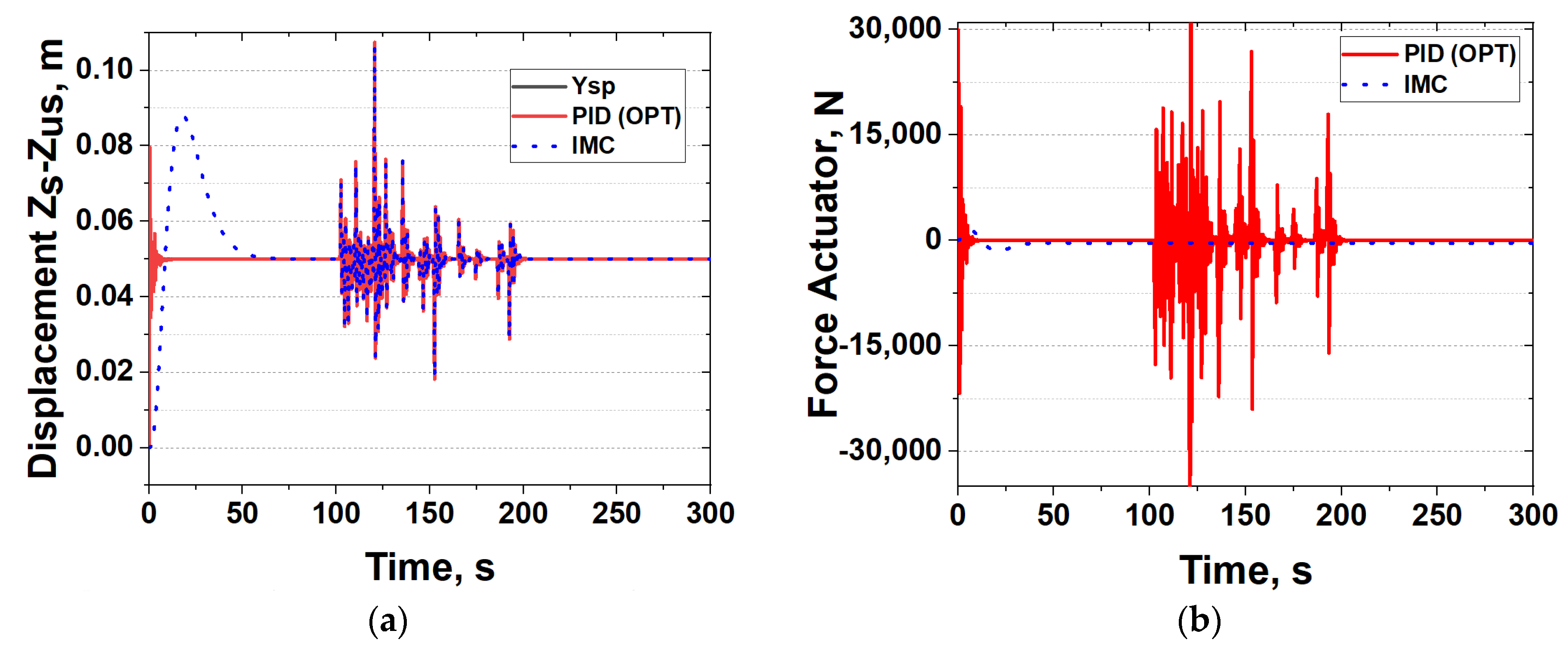
The core aim of this study was the establishment of a feedback control system for an active suspension system. The open loop simulations revealed that the presence of disturbances induces high overshoots and continuous oscillations that are persistent in time. With this indication in mind, the need for a control system design was verified. Next, the evaluation and comparison of three sets of feedback controllers took place: (a) P, PI and PID tuned controllers via the Ziegler–Nichols and Tyreus–Luyben methods, (b) an optimally tuned PID controller via genetic algorithms and (c) an internal model controller. Through a set of simulation scenarios that involved set-point tracking with and without the effect of bumps and holes (road disturbances), it was shown that the optimally tuned PID and IMC controllers exhibit a superior performance in terms of ride comfort and minimum control actions. Among the two, the IMC controller exhibited the lowest (overall) action from the actuator, whereas the optimal PID controller presented the best results for the performance criteria of errors, peak overshoots and settling and rise times, but with extreme mechanical effort from the actuator elements.

Future studies regarding the effective control of active suspension systems should involve the application of advanced methodologies such as model predictive control. This way, the optimal action from the actuator could be applied in order to sustain a predefined trajectory despite emerged disturbances. Furthermore, the application of the most crucial research findings could be implemented using lab hardware equipment, which could involve a similar mechanical structure accompanied by automation utilities.

References

1. Petri, A.-M.; Petreuș, D.M. Adaptive Cruise Control in Electric Vehicles with Field-Oriented Control. Appl. Sci. 2022, 12, 7094. [Google Scholar] [CrossRef]
2. Brugnolli, M.M.; Angelico, B.A.; Lagana, A.A.M. Predictive Adaptive Cruise Control Using a Customized ECU. IEEE Access 2019, 7, 55305–55317. [Google Scholar] [CrossRef]
3. Chen, C.; Guo, J.; Guo, C.; Chen, C.; Zhang, Y.; Wang, J. Adaptive Cruise Control for Cut-In Scenarios Based on Model Predictive Control Algorithm. Appl. Sci. 2021, 11, 5293. [Google Scholar] [CrossRef]
4. Yang, W.; Chen, Y.; Su, Y. A Double-Layer Model Predictive Control Approach for Collision-Free Lane Tracking of On-Road Autonomous Vehicles. Actuators 2023, 12, 169. [Google Scholar] [CrossRef]
5. Tang, B.; Hu, Z.; Jiang, H.; Yin, Y.; Yang, Z. Dynamic Lane Tracking Control of the Commercial Vehicle Based on RMPC Algorithm Considering the State of Preceding Vehicle. Machines 2022, 10, 534. [Google Scholar] [CrossRef]
6. Shafiei, B. A Review on PID Control System Simulation of the Active Suspension System of a Quarter Car Model While Hitting Road Bumps. J. Inst. Eng. Ser. C 2022, 103, 1001–1011. [Google Scholar] [CrossRef]
7. Daniyan, I.A.; Mpofu, K.; Osadare, D.F. Design and simulation of a controller for an active suspension system of a rail car. Cogent. Eng. 2018, 5, 1–15. [Google Scholar] [CrossRef]
8. Gowda, D.V.; Chakrasali, S. Comparative Analysis of Passive and Semi-Active Suspension System for Quarter Car Model Using PID Controller. 2014. Available online: https://www.researchgate.net/publication/276276510 (accessed on 1 September 2023).
9. Ding, X.; Li, R.; Cheng, Y.; Liu, Q.; Liu, J. Design of and Research into a Multiple-Fuzzy PID Suspension Control System Based on Road Recognition. Processes 2021, 9, 2190. [Google Scholar] [CrossRef]
10. Han, S.-Y.; Dong, J.-F.; Zhou, J.; Chen, Y.-H. Adaptive Fuzzy PID Control Strategy for Vehicle Active Suspension Based on Road Evaluation. Electronics 2022, 11, 921. [Google Scholar] [CrossRef]
11. Al-Zughaibi, A.I. Controller Design for Active Suspension System of ¼ Car with Unknown Mass and Time-Delay. Available online: https://www.researchgate.net/publication/280934598 (accessed on 1 September 2023).
12. Papaioannou, G.; Ning, D.; Jerrelind, J.; Drugge, L. A K-Seat-Based PID Controller for Active Seat Suspension to Enhance Motion Comfort. SAE Int. J. Connect. Autom. Veh. 2022, 5, 189–199. [Google Scholar] [CrossRef]
13. Zhu, J.; Zhao, D.; Liu, S.; Zhang, Z.; Liu, G.; Chang, J. Integrated Control of Spray System and Active Suspension Systems Based on Model-Assisted Active Disturbance Rejection Control Algorithm. Mathematics 2022, 10, 3391. [Google Scholar] [CrossRef]
14. Dahunsi, O.A.; Dahunsi, O.A.; Pedro, J.O. Neural Network-Based Identification and Approximate Predictive Control of a Servo-Hydraulic Vehicle Suspension System Ergonomic Evaluation of Dynamic and Post Effects of Vibration on Earthmoving EQUIPMENT Operators View Project Neural Network-Based Identification and Approximate Predictive Control of a Servo-Hydraulic Vehicle Suspension System. 2010. Available online: https://www.researchgate.net/publication/49586591 (accessed on 1 September 2023).
15. Kim, J.; Lee, T.; Kim, C.J.; Yi, K. Model predictive control of a semi-active suspension with a shift delay compensation using preview road information. Control Eng. Pract. 2023, 137, 105584. [Google Scholar] [CrossRef]
16. Zhang, N.; Yang, S.; Wu, G.; Ding, H.; Zhang, Z.; Guo, K. Fast Distributed Model Predictive Control Method for Active Suspension Systems. Sensors 2023, 23, 3357. [Google Scholar] [CrossRef]
17. Payakkawan, P.; Klomkarn, K.; Sooraksa, P. Dual-line PID controller based on PSO for speed control of DC motors. In Proceedings of the 2009 9th International Symposium on Communications and Information Technology, ISCIT 2009, Incheon, Republic of Korea, 28–30 September 2009; pp. 134–139. [Google Scholar] [CrossRef]
18. Mat, M.H.; Darns, I.Z.M. Self-tuning PID controller for active suspension system with hydraulic actuator. In Proceedings of the IEEE Symposium on Computers and Informatics, ISCI 2013, Langkawi, Malaysia, 7–9 April 2013; IEEE Computer Society: Piscataway, NJ, USA, 2013; pp. 86–91. [Google Scholar] [CrossRef]
19. Zeng, Q.; Zhao, J. Event-triggered controller design for active suspension systems: An adaptive backstepping method with error-dependent gain. Control Eng. Pract. 2023, 136, 105547. [Google Scholar] [CrossRef]
20. Jeong, Y.; Sohn, Y.; Chang, S.; Yim, S. Design of Static Output Feedback Controllers for an Active Suspension System. IEEE Access 2022, 10, 26948–26964. [Google Scholar] [CrossRef]
21. Liu, J.; Liu, J.; Li, Y.; Wang, G.; Yang, F. Study on Multi-Mode Switching Control Strategy of Active Suspension Based on Road Estimation. Sensors 2023, 23, 3310. [Google Scholar] [CrossRef]
22. Kozek, M.; Smoter, A.; Lalik, K. Neural-Assisted Synthesis of a Linear Quadratic Controller for Applications in Active Suspension Systems of Wheeled Vehicles. Energies 2023, 16, 1677. [Google Scholar] [CrossRef]
23. Alvarez-Sánchez, E. A Quarter-Car Suspension System: Car Body Mass Estimator and Sliding Mode Control. Procedia Technol. 2013, 7, 208–214. [Google Scholar] [CrossRef]
24. Nguyen, T.A. Research on the Sliding Mode—PID control algorithm tuned by fuzzy method for vehicle active suspension. Forces Mech. 2023, 11, 100206. [Google Scholar] [CrossRef]
25. Fu, Z.-J.; Dong, X.-Y. H∞ optimal control of vehicle active suspension systems in two time scales. Automatika 2021, 62, 284–292. [Google Scholar] [CrossRef]
26. Chen, L.; Xu, X.; Liang, C.; Jiang, X.-W.; Wang, F. Semi-active control of a new quasi-zero stiffness air suspension for commercial vehicles based on H2H state feedback. J. Vib. Control. 2023, 29, 1910–1926. [Google Scholar] [CrossRef]
27. Ahmad, I.; Ge, X.; Han, Q.-L. Communication-Constrained Active Suspension Control for Networked In-Wheel Motor-Driven Electric Vehicles with Dynamic Dampers. IEEE Trans. Intell. Veh. 2022, 7, 590–602. [Google Scholar] [CrossRef]
28. Merah, A.; Hartani, K.; Yazid, N.E.H.; Chikouche, T.M. New Integrated Full Vehicle Suspension System for Improvements in Vehicle Ride Comfort and Road Holding. SAE Int. J. Veh. Dyn. Stab. NVH 2022, 6, 267–281. [Google Scholar] [CrossRef]
29. Azmi, R.; Mirzaei, M.; Habibzadeh-Sharif, A. A novel optimal control strategy for regenerative active suspension system to enhance energy harvesting. Energy Convers. Manag. 2023, 291, 117277. [Google Scholar] [CrossRef]
30. Liu, Y.J.; Zeng, Q.; Liu, L.; Tong, S. An Adaptive Neural Network Controller for Active Suspension Systems with Hydraulic Actuator. IEEE Trans. Syst. Man Cybern. Syst. 2020, 50, 5351–5360. [Google Scholar] [CrossRef]
31. Qu, Z.; Liu, J.; Li, Y.; Yang, F.; Liu, J. Study on Multi-Mode Switching Control of Intelligent Suspension under Full Road Section. Processes 2023, 11, 1776. [Google Scholar] [CrossRef]
32. He, X.L.; Chen, J.; Tang, D.Y.; Peng, S.; Tang, B.B. Using an Inerter-Based Suspension to Reduce Carbody Flexible Vibration and Improve Riding-Comfort. SAE Int. J. Veh. Dyn. Stab. NVH 2023, 7, 137–151. [Google Scholar] [CrossRef]
33. Ikeda, K.; Kuroda, J.; Uchino, D.; Ogawa, K.; Endo, A.; Kato, T.; Kato, H.; Narita, T. A Study of a Ride Comfort Control System for Ultra-Compact Vehicles Using Biometric Information. Appl. Sci. 2022, 12, 7425. [Google Scholar] [CrossRef]
34. Kaldas, M.M.; Soliman, A.M.A.; Abdallah, S.A.; Mohammad, S.S.; Amien, F.F. Road Preview Control for Active Suspension System. SAE Int. J. Veh. Dyn. Stab. NVH 2022, 6, 371–383. [Google Scholar] [CrossRef]
35. Abbas, G.; Asad, M.U.; Gu, J.; Alelyani, S.; Balas, V.E.; Hussain, M.R.; Farooq, U.; Awan, A.B.; Raza, A.; Chang, C. Multivariable unconstrained pattern search method for optimizing digital pid controllers applied to isolated forward converter. Energies 2021, 14, 77. [Google Scholar] [CrossRef]
36. The MathWorks Inc. Optimization Toolbox, version 9.4 (R2022b); The MathWorks Inc.: Natick, MA, USA, 2022.
37. Bequette, B. Process Control: Modeling, Design, and Simulation; Prentice Hall Press: Upper Saddle River, NJ, USA, 2002. [Google Scholar]
38. Nise, N.S. Control Systems Engineering, 8th ed.; Wiley: Hoboken, NJ, USA, 2019. [Google Scholar]
Figure 1. A quarter-car model of the suspension system.
Processes 11 02715 g001
Figure 2. Active suspension system of a (1/4) quarter car.
Processes 11 02715 g002
Figure 4. Open loop simulations for scenarios A–D: displacement of the suspension system as y = ZsZus (a) constant force without disturbance, (b) variable force without disturbance, (c) constant force with short-term disturbance and (d) constant force with long-term disturbance.
Processes 11 02715 g004
Figure 5. Feedback control for the active suspension system.
Processes 11 02715 g005
Figure 8. Comparison of P and PI controllers during scenario 1: (a) displacement of the active suspension system and (b) force actuator control action.
Processes 11 02715 g008
Figure 9. Comparison of PID controllers during scenario 1: (a) displacement of the active suspension system and (b) force actuator control action.
Processes 11 02715 g009
Figure 10. Comparison of P and PI controllers during scenario 2: (a) displacement of the active suspension system and (b) force actuator control action.
Processes 11 02715 g010
Figure 11. Comparison of PID controllers during scenario 2: (a) displacement of the active suspension system and (b) force actuator control action.
Processes 11 02715 g011
Figure 12. Comparison of optimal PID and IMC controllers during scenario 1: (a) displacement of the active suspension system and (b) force actuator control action.
Processes 11 02715 g012
Figure 13. Comparison of optimal PID and IMC controllers during modified scenario 2: (a) displacement of the active suspension system and (b) force actuator control action.
Processes 11 02715 g013