On Unit Exponential Pareto Distribution for Modeling the Recovery Rate of COVID-19

Abstract

In 2019, a new lethal and mutant virus (COVID-19) spread around the world, causing the deaths of millions of people. COVID-19 demonstrates that scientists are involved in significant research efforts to face bacteria with less effort than that dedicated to viruses. Since then, engineers and bio-materials scientists have been trying to develop antiviral research and find a suitable effective medication. Strategies and opportunities for interference diagnostics, treatment strategies, and predicting future factors became mandatory. From a statistical point of view, estimating and modelling these factors play an important role in preventing future viral epidemics. In this article, modelling the recovery rate of COVID-19 is investigated through a new distribution which is called the unit exponential Pareto distribution. The new continuous distribution with three parameters displays a prominent level of flexibility to model decreasing, symmetric, and asymmetric data with a monotone failure rate. The recovery rates of COVID-19 in Turkey and France were examined; moreover, milk production data and components’ failure rates are presented for data modeling. The obtained results proved the superiority of the newly suggested model compared to other unit-based distributions. Several statistical features are studied such as the quantile function, the moments, the moment-generating function, some entropy measures, the ordered statistics, the stress–strength, and stochastic ordering. Two classical estimation methods are used in addition to the Bayesian method. The statistical features and estimation analysis are evaluated using numerical and simulation techniques. As a result, we obtain the efficiency of using the Bayesian method over the classical ones, with respect to the bias, average squared error, and the length of confidence intervals for the unknown parameters.

1. Introduction

Since the spread of the COVID-19 pandemic in early 2020, a clear deficiency appeared in humans’ ability to reduce the spread of infection caused by this viral disease and to afford suitable medication for patients. Consequently, health organizations faced a challenging situation and health crises emerged. A few months later, China recorded a high death rate with a very low recovery rate. Since that, the knowledge about this novel virus has been developed, but is still not enough. An essential need for new diagnostics and medication to reduce or prevent virus transmission must be considered. Different vaccination types have been developed, in addition to applying the precautionary measures in many countries that resulted in increasing the recovery rate and reducing death cases, see [1]. Biomaterials science has made a great contribution to the enhancement of new and personal protective tools, vaccines, and drug delivery which can be used to treat COVID-19 and its side effects. Furthermore, tissue engineers and cell-biology models can have a great influence on inspecting the disease, testing, and improving new vaccines, see [2]. One of the main factors that indicate the improvement of the treatment process is the recovery rate; hence, modelling this factor is important and it will lead to many useful results and the development of biomedical research related to COVID-19 or any other viral disease. Modelling real-life phenomena from a statistical point of view have been widely considered in the literature. For example, one may refer to the book [3], in which the author studied the factors affecting the degradation of an organic coating by forecasting the remaining lifetime of the coating. In many scientific fields, statistical models are required to describe the trend of the data under consideration. For the purpose of modeling real data, several new generators of distributions appeared in the literature. The most attractive ones are the beta and Kumaraswamy distributions, see [4,5]. However, since more data became available and spread quickly, there is a persistent need for new families of distributions. A unit distribution is a type of distribution that is usually used to model the extreme values in a population. It is characterized by a power-law relationship, where the probability of observing a value within a certain range decreases exponentially as the value increases. Consequently, more studies about unit modeling appeared in the literature. Generally, new unit distributions are formulated by transforming some familiar continuous distributions, which are more flexible than the original ones, without adding new parameters. For more examples of unit distributions, one may refer to the unit Weibull [6,7], the unit Gompertz [8], the unit Birnbaum–Saunders [9], the unit inverse Gaussian [10], the unit generalized half normal [11], the unit Rayleigh [12], the unit Burr-XII [13], the unit Chen [14], and the unit power Weibull [15] distributions.

In the literature, the Pareto (P) distribution is a well-known statistical continuous model that describes heavy-tailed data. Ref. [16] explained the P distribution’s applications in modeling earthquakes, forest-fire areas, and oil- and gas-field sizes. Various generalizations appeared in the research work, which emphasizes the flexibility of the P model. For example, the Weibull-P distribution [17], the Gamma-P distribution [18], the beta-P distribution [19], the beta generalized P distribution [20], the Kumaraswamy exponentiated P distribution [21] and a new Weibull-P distribution [22]. One may refer to [23,24,25,26] for more generalized P distributions.

Some unit models were obtained using other transformation methods, see, for example, [27,28,29,30,31,32].

Ref. [33] studied a new model based on the exponential and P distributions. The cumulative density function (CDF) and the probability density function (pdf) of the exponential P distribution (EPD) are given, respectively, as

$$F\left(y\right)=1-e^{-\lambda {\left(\frac{y}{\beta }\right)}^{\alpha }},$$

(1)

and

$$f\left(y\right)=\frac{\alpha \lambda }{\beta }{\left(\frac{y}{\beta }\right)}^{\alpha -1}{e}^{-\lambda {\left(\frac{y}{\beta }\right)}^{\alpha }},$$

(2)

where $y>0$, $\alpha$ is a positive shape parameter, and $\beta$ and $\lambda$ are positive scale parameters. The EPD is a very flexible model and has many applications in different fields. However, in this paper, we introduce a new statistical model that has more flexibility than the EPD in many different fields and the application section recommended our claims. The newly suggested model is called the unit exponential Pareto distribution.

One of the main motivations for using the unit exponential Pareto distribution is its ability to capture the long-tailed nature of many real-world data sets. In addition to its ability to model long-tailed data, the unit exponential Pareto distribution is also useful for identifying patterns and trends in data. By analyzing the shape of the distribution, insight can be gained into the underlying factors that drive the data and informed decisions made about how to best allocate resources or make predictions about future observations.

The basic goal of this work is to introduce the new unit exponential Pareto distribution (UEPD), study its statistical properties, and explore the ability of UEPD by applying it to three real-life data examples. The stimulus for studying the UEPD are: (i) UEPD is a distinguished model since it is constructed on the bases of the unit interval [0,1] rather than the positive real numbers; (ii) it has remarkable flexibility with respect to tail features; hence, it is used in risk evaluation theory with relatively improved outputs; and (iii) the potency of the new mixture of the well-known exponential and Pareto distributions appears in modeling and fitting many real-life data with relatively fewer errors than other competitive models. This new model proves the suitability of fit to the COVID-19 recovery rate in two countries, Turkey and France, during the pandemic, in addition to the modeling production rate and failure times of components as an application in economic and engineering fields.

The rest of the article is presented as follows: Section 2 investigates the UEPD and discusses the basic properties of this distribution. In Section 3, some important distributional and statistical features of the UEPD are studied, such as the quantile function ($Q{U}_{N}F$), moments ($M_O$s), moment-generating function ($M_{O}GF$), some entropy measures, order statistics ($O_S$), stress–strength ($S_S$), and stochastic ordering ($S_{OR}$). Classical estimation methods are discussed in Section 4, while the Bayesian approach is implemented in Section 5. Section 6 presents the results of examining three real-skewed data sets. Section 7 investigates the performance of the suggested estimation techniques using Monte Carlo simulations. Finally, Section 8 summarizes the relevant conclusions and remarks.

2. Unit Exponential Pareto Distribution

Assume Y is a random variable ($R{V}_R$) which follows the EPD with parameters $\alpha ,\beta$ and $\lambda$. Applying the transformation $Y=\frac{X}{1-X}$ then, the new unit distribution is created. The pdf and the CDF of the transformed variable X are provided via

$$f\left(x\right)=\frac{\alpha \lambda }{\beta }{\left(\frac{x}{\beta (1-x)}\right)}^{\alpha -1}{e}^{-\lambda {\left(\frac{x}{\beta (1-x)}\right)}^{\alpha }},$$

(3)

and

$$F\left(x\right)=1-e^{-\lambda {\left(\frac{x}{\beta (1-x)}\right)}^{\alpha }},$$

(4)

where $0<x<1$, $\alpha >0$ is the shape parameter and $\beta$ and $\lambda$ are non-negative scale parameters.

Figure 1 represents the shape of the UEPD distribution, which is decreasing, upside down with uni-modal, skewed to the left, and symmetric for some selected parameter values.

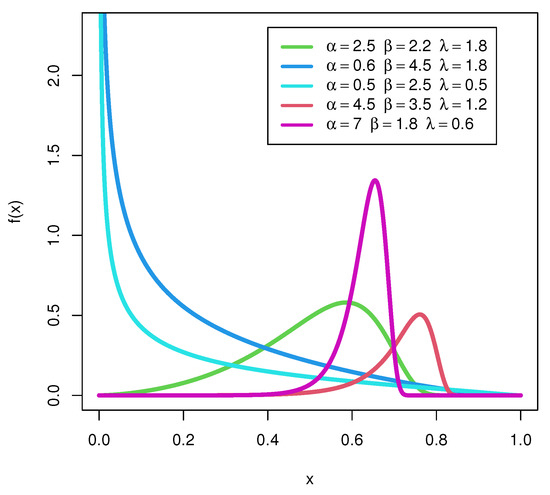
Figure 1. pdf plots of UEPD.

The survival function (SF) is a function that provides the probability that a particular object will survive after a specific time. The term survival function is extensively used in human mortality to show the survival time of a patient beyond a specific time. Reliability analysis is used to show the performance of electric devices beyond a fixed time. The SF for the UEPD is provided as

$$S\left(x\right)=e^{-\lambda {\left(\frac{x}{\beta (1-x)}\right)}^{\alpha }.}$$

(5)

The hazard function (HF) for the UEPD is obtained as

$$h\left(x\right)=\frac{\alpha \lambda }{\beta }{\left(\frac{x}{\beta (1-x)}\right)}^{\alpha -1}.$$

(6)

Figure 2 depicts the HFs of the UEPD distribution. It is noticed that the distribution has decreasing HFs if $\alpha <1$, while it has increasing HFs for $\alpha >1$, and is constant for $\alpha =1$, with different values for the other two parameters. This shows the flexibility of the UEPD. The cumulative HF of the UEPD is obtained by

$$H\left(x\right)={\displaystyle \underset{0}{\overset{x}{\int }}}\frac{\alpha \lambda }{\beta }{\left(\frac{t}{\beta (1-t)}\right)}^{\alpha -1}dt=\lambda {\left(\frac{x}{\beta (1-x)}\right)}^{\alpha }.$$

(7)

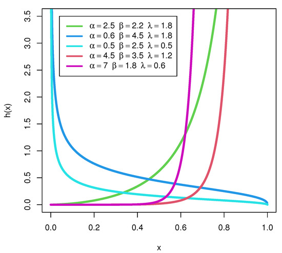
Figure 2. Hazard plots of UEPD with different values of parameters.

The reversed HF (RHF) is another important tool in reliability analysis and it is calculated as

$$r\left(x\right)=\frac{f\left(x\right)}{F\left(x\right)}=\frac{\frac{\alpha \lambda }{\beta }{\left(\frac{x}{\beta (1-x)}\right)}^{\alpha -1}{e}^{-\lambda {\left(\frac{x}{\beta (1-x)}\right)}^{\alpha }}}{1-e^{-\lambda {\left(\frac{x}{\beta (1-x)}\right)}^{\alpha }}}.$$

(8)

3. Statistical Properties

Some important structural and statistical properties of the UEPD are investigated in this section.

3.1. Quantile Function

The $Q{U}_{N}F$ of the UEPD is a useful tool to perform a simulated sample and it can be calculated by solving $F\left(x\right)=u$ with respect to x, where $u\sim Uniform(0,1)$, that is, $u=$$1-e^{-\lambda {\left(\frac{x}{\beta (1-x)}\right)}^{\alpha }}$. The simplified form of the $Q{U}_{N}F$ of the UEPD is provided by

$$x={\left[1+\frac{{(-\lambda )}^{\frac{1}{\alpha }}}{\beta }{(ln(1-u))}^{\frac{-1}{\alpha }}\right]}^{-1}.$$

(9)

The $q$th quartile function of the UEPD is defined as

$$x_q={\left[1+\frac{{(-\lambda )}^{\frac{1}{\alpha }}}{\beta }{(ln(1-q))}^{\frac{-1}{\alpha }}\right]}^{-1}.$$

(10)

For $q=0.5$, Equation $\left(10\right)$ reveals the median of the UEPD

$$x_{0.5}={\left[1+\frac{{(-\lambda )}^{\frac{1}{\alpha }}}{\beta }{(ln\left(0.5\right))}^{\frac{-1}{\alpha }}\right]}^{-1}.$$

(11)

3.2. Moments

We derive the rth Moment ($M_O$) for the UEPD. The first four $M_O$s are the most important to describe the shape and monotonicity of the distribution curve. Suppose X via a $R{V}_R$ that follows $UEPD$($\alpha ,\beta ,\lambda$); then, the rth $M_O$ about the origin of the UEPD is provided via

$${\mu }_r^{{}^{/}}={\int }_0^1{x}^{r}f(x;\alpha ,\beta ,\lambda )dx.$$

(12)

By substituting Equation (3) into Equation (12), we obtain

$${\mu }_r^{{}^{/}}={\int }_0^1{x}^r\frac{\alpha \lambda }{\beta }{\left(\frac{x}{\beta (1-x)}\right)}^{\alpha -1}{e}^{-\lambda {\left(\frac{x}{\beta (1-x)}\right)}^{\alpha }}dx,$$

where $z=\frac{x}{\beta (1-x)},$

$${\mu }_r^{{}^{/}}=\frac{{\lambda }^{\frac{2}{\alpha }}}{{\beta }^2}{\int }_0^{\infty }{\left[1+\frac{{\lambda }^{\frac{1}{\alpha }}}{\beta }{z}^{\frac{-1}{\alpha }}\right]}^{-(r+2)}{e}^{-z}dz.$$

Using the binomial expansion on

$${\left[1+\frac{{\lambda }^{\frac{1}{\alpha }}}{\beta }{z}^{\frac{-1}{\alpha }}\right]}^{-(r+2)}=\underset{i=0}{\sum ^{\infty }}\left(\genfrac{}{}{0pt}{}{-r-2}{i}\right)\frac{{\lambda }^{\frac{i}{\alpha }}}{{\beta }^i}{z}^{-\frac{i}{\alpha }},$$

we obtained an expression for the moment as

$$\begin{array}{cc}\hfill {\mu }_r^{{}^{/}}& =\frac{{\lambda }^{\frac{2}{\alpha }}}{{\beta }^2}\sum _{i=0}^{\infty }\left(\genfrac{}{}{0pt}{}{-r-2}{i}\right)\frac{{\lambda }^{\frac{i}{\alpha }}}{{\beta }^i}{\int }_0^{\infty }{z}^{-\frac{i}{\alpha }}{e}^{-z}dz\hfill \\ & =\frac{{\lambda }^{\frac{2}{\alpha }}}{{\beta }^2}\sum _{i=0}^{\infty }\left(\genfrac{}{}{0pt}{}{-r-2}{i}\right)\frac{{\lambda }^{\frac{i+2}{\alpha }}}{{\beta }^{i+2}}\mathsf{\Gamma }(1-\frac{i}{\alpha }).\hfill \end{array}$$

It is important to note that the $M_O$s exist only when $\frac{i}{\alpha }<1.$ In particular, the first four $M_O$s of UEPD are written as

$$\begin{array}{cc}\hfill & {\mu }_1^{{}^{/}}=\sum _{i=0}^{\infty }\left(\genfrac{}{}{0pt}{}{-3}{i}\right)\frac{{\lambda }^{\frac{i+2}{\alpha }}}{{\beta }^{i+2}}\mathsf{\Gamma }(1-\frac{i}{\alpha }),\hfill \\ & {\mu }_2^{{}^{/}}=\sum _{i=0}^{\infty }\left(\genfrac{}{}{0pt}{}{-4}{i}\right)\frac{{\lambda }^{\frac{i+2}{\alpha }}}{{\beta }^{i+2}}\mathsf{\Gamma }(1-\frac{i}{\alpha }),\hfill \\ & {\mu }_3^{{}^{/}}=\sum _{i=0}^{\infty }\left(\genfrac{}{}{0pt}{}{-5}{i}\right)\frac{{\lambda }^{\frac{i+2}{\alpha }}}{{\beta }^{i+2}}\mathsf{\Gamma }(1-\frac{i}{\alpha })\hfill \end{array}$$

and

$${\mu }_4^{{}^{/}}=\sum _{i=0}^{\infty }\left(\genfrac{}{}{0pt}{}{-6}{i}\right)\frac{{\lambda }^{\frac{i+2}{\alpha }}}{{\beta }^{i+2}}\mathsf{\Gamma }(1-\frac{i}{\alpha }).$$

As a result, the mean and variance are derived by

$$\mu =\sum _{i=0}^{\infty }\left(\genfrac{}{}{0pt}{}{-3}{i}\right)\frac{{\lambda }^{\frac{i+2}{\alpha }}}{{\beta }^{i+2}}\mathsf{\Gamma }(1-\frac{i}{\alpha }),$$

and

$$Var\left(x\right)=\sum _{i=0}^{\infty }\left(\genfrac{}{}{0pt}{}{-4}{i}\right)\frac{{\lambda }^{\frac{i+2}{\alpha }}}{{\beta }^{i+2}}\mathsf{\Gamma }(1-\frac{i}{\alpha })-{\left(\stackrel{\infty }{{\sum }_{i=0}}\left(\genfrac{}{}{0pt}{}{-3}{i}\right)\frac{{\lambda }^{\frac{i+2}{\alpha }}}{{\beta }^{i+2}}\mathsf{\Gamma }(1-\frac{i}{\alpha })\right)}^2.$$

Table 1 shows some numerical values of the first four moments $E\left(X\right)$, $E\left(X^2\right)$, $E\left(X^3\right)$, $E\left(X^4\right)$; the variance (var); skewness (SK); kurtosis (KU); coefficient of variation (CV) and index of dispersion (ID).

Table 1. Some numerical values of moments for the UEPD at $\lambda =0.5$.

$\mathit{\beta }$	$\mathit{\alpha }$	$\mathit{E}\left(\mathit{X}\right)$	$\mathit{E}\left({\mathit{X}}^2\right)$	$\mathit{E}\left({\mathit{X}}^3\right)$	$\mathit{E}\left({\mathit{X}}^4\right)$	var	SK	KU	CV	ID
0.8	1.5	0.111	0.05	0.025	0.013	0.037	1.542	4.034	1.744	0.337
	2.0	0.12	0.054	0.026	0.013	0.039	1.31	3.167	1.657	0.329
	2.5	0.1250	0.0560	0.0270	0.0130	0.0400	1.1750	2.7090	1.6100	0.3230
	3.0	0.1280	0.0570	0.0270	0.0130	0.0410	1.0890	2.4370	1.5810	0.3200
	4.0	0.1310	0.0590	0.0270	0.0130	0.0420	0.9920	2.1440	1.5510	0.3160
1.2	1.5	0.0930	0.0470	0.0260	0.0160	0.0380	1.9760	5.5650	2.1080	0.4130
	2.0	0.1000	0.0520	0.0290	0.0170	0.0420	1.7940	4.6600	2.0540	0.4200
	2.5	0.1030	0.0550	0.0300	0.0170	0.0440	1.6920	4.1790	2.0270	0.4250
	3.0	0.1060	0.0560	0.0310	0.0180	0.0450	1.6300	3.8930	2.0110	0.4270
	4.0	0.1080	0.0580	0.0320	0.0180	0.0470	1.5630	3.5860	1.9950	0.4310
1.5	1.5	0.0820	0.0440	0.0260	0.0160	0.0370	2.2640	6.8140	2.3550	0.4540
	2.0	0.0870	0.0480	0.0290	0.0180	0.0410	2.1160	5.9330	2.3280	0.4710
	2.5	0.0890	0.0510	0.0300	0.0190	0.0430	2.0370	5.4690	2.3180	0.4810
	3.0	0.0910	0.0530	0.0310	0.0190	0.0440	1.9900	5.1960	2.3130	0.4870
	4.0	0.1250	0.0450	0.0180	0.0008	0.0290	1.0900	2.9300	1.3630	0.2320

3.3. The Moment-Generating Function

The $M_O$-generating function of the UEPD can be calculated from

$$M_X\left(t\right)={\int }_0^1{e}^{tx}f(x;\alpha ,\beta ,\lambda )dx.$$

(13)

As a result, using the Taylor series to extend $M_X\left(t\right)$ produces

$$M_X\left(t\right)=\underset{r=0}{{\displaystyle \sum }^{\infty }}\frac{t^r}{r!}{\int }_0^1{x}^{r}f(x;\alpha ,\beta ,\lambda )dx.$$

$$M_X\left(t\right)=\sum _{i=r=0}^{\infty }\frac{t^r}{r!}\left(\genfrac{}{}{0pt}{}{-r-2}{i}\right)\frac{{\lambda }^{\frac{i+2}{\alpha }}}{{\beta }^{i+2}}\mathsf{\Gamma }(1-\frac{i}{\alpha }).$$

(14)

3.4. Different Types of Entropy

Entropy measures are important measures in reliability and risk-analysis studies. It has been used in a wide range of applied biological, medical and physical fields.

3.4.1. Rényi Entropy

The essential shape of the distribution is measured using Rényi entropy (RE) [34] and it is provided by

$$R_{\nu }=\frac{1}{1-\nu }log\left[{\displaystyle \underset{0}{\overset{1}{\int }}}{\left(f(x;\alpha ,\beta ,\lambda )\right)}^{\nu }dx\right],\nu >0,\nu \ne 1.$$

(15)

For UEPD, Rényi entropy is obtained as

$$R_{\nu }=\frac{1}{1-\nu }log\left[{\displaystyle \underset{0}{\overset{1}{\int }}}\frac{{\alpha }^{\nu }{\lambda }^{\nu }}{{\beta }^{\nu }}{\left(\frac{x}{\beta (1-x)}\right)}^{\nu \alpha -\nu }{e}^{-\nu \lambda {\left(\frac{x}{\beta (1-x)}\right)}^{\alpha }}dx\right],$$

where $z=\nu \lambda {\left(\frac{x}{\beta (1-x)}\right)}^{\alpha }.$ Then

$$\begin{array}{cc}\hfill R_{\nu }& =\frac{1}{1-\nu }log\left[\sum _{i=0}^{\infty }\left(\genfrac{}{}{0pt}{}{-2}{i}\right)\frac{{\alpha }^{\nu -1}{\lambda }^{\frac{\nu -i-1}{\alpha }}{\nu }^{\frac{\nu -\nu \alpha -i-1}{\alpha }}}{{\beta }^{\nu -i-1}}{\int }_0^{\infty }{z}^{\frac{i+\nu \alpha -\nu -\alpha -1}{\alpha }}{e}^{-z}dz\right]\hfill \\ \hfill & =\frac{1}{1-\nu }log\left[\sum _{i=0}^{\infty }\left(\genfrac{}{}{0pt}{}{-2}{i}\right)\frac{{\alpha }^{\nu -1}{\lambda }^{\frac{\nu -i-1}{\alpha }}{\nu }^{\frac{\nu -\nu \alpha -i-1}{\alpha }}}{{\beta }^{\nu -i-1}}\mathsf{\Gamma }\left(\frac{i+\nu \alpha -\nu -1}{\alpha }\right)\right].\hfill \end{array}$$

3.4.2. Havrda and Charvat Entropy

The Havrda and Charvat entropy (HCE) [35] measure is provided via

$$H{C}_{\nu }=\frac{1}{2^{1-\nu }-1}\left[{\left({\displaystyle \underset{0}{\overset{1}{\int }}}{\left(f(x;\alpha ,\beta ,\lambda )\right)}^{\nu }dx\right)}^{\frac{1}{\nu }}-1\right],\nu >0,\nu \ne 1.$$

(16)

For UEPD, Havrda and Charvat entropy is obtained as

$$H{C}_{\nu }=\frac{1}{2^{1-\nu }-1}\left[{\left({\displaystyle \underset{0}{\overset{1}{\int }}}\frac{{\alpha }^{\nu }{\lambda }^{\nu }}{{\beta }^{\nu }}{\left(\frac{x}{\beta (1-x)}\right)}^{\nu \alpha -\nu }{e}^{-\nu \lambda {\left(\frac{x}{\beta (1-x)}\right)}^{\alpha }}dx\right)}^{\frac{1}{\nu }}-1\right],$$

where $z=\nu \lambda {\left(\frac{x}{\beta (1-x)}\right)}^{\alpha }.$ Then

$$\begin{array}{cc}\hfill H{C}_{\nu }& =\frac{1}{2^{1-\nu }-1}\left[{\left(\sum _{i=0}^{\infty }\left(\genfrac{}{}{0pt}{}{-2}{i}\right)\frac{{\alpha }^{\nu -1}{\lambda }^{\frac{\nu -i-1}{\alpha }}{\nu }^{\frac{\nu -\nu \alpha -i-1}{\alpha }}}{{\beta }^{\nu -i-1}}{\int }_0^{\infty }{z}^{\frac{i+\nu \alpha -\nu -\alpha -1}{\alpha }}{e}^{-z}dz\right)}^{\frac{1}{\nu }}-1\right]\hfill \\ \hfill & =\frac{1}{2^{1-\nu }-1}\left[{\left(\sum _{i=0}^{\infty }\left(\genfrac{}{}{0pt}{}{-2}{i}\right)\frac{{\alpha }^{\nu -1}{\lambda }^{\frac{\nu -i-1}{\alpha }}{\nu }^{\frac{\nu -\nu \alpha -i-1}{\alpha }}}{{\beta }^{\nu -i-1}}\mathsf{\Gamma }\left(\frac{i+\nu \alpha -\nu -1}{\alpha }\right)\right)}^{\frac{1}{\nu }}-1\right].\hfill \end{array}$$

3.4.3. Tsallis Entropy

The Tsallis entropy (TE) [36] measure is provided by

$$T_{\nu }=\frac{1}{\nu -1}\left[1-{\displaystyle \underset{0}{\overset{1}{\int }}}{\left(f(x;\alpha ,\beta ,\lambda )\right)}^{\nu }dx\right],\nu >0,\nu \ne 1.$$

(17)

For UEPD, Tsallis entropy is obtained as

$$T_{\nu }=\frac{1}{\nu -1}\left[1-{\displaystyle \underset{0}{\overset{1}{\int }}}\frac{{\alpha }^{\nu }{\lambda }^{\nu }}{{\beta }^{\nu }}{\left(\frac{x}{\beta (1-x)}\right)}^{\nu \alpha -\nu }{e}^{-\nu \lambda {\left(\frac{x}{\beta (1-x)}\right)}^{\alpha }}dx\right],$$

where $z=\nu \lambda {\left(\frac{x}{\beta (1-x)}\right)}^{\alpha }.$ Then

$$\begin{array}{cc}\hfill T_{\nu }& =\frac{1}{\nu -1}\left[1-\sum _{i=0}^{\infty }\left(\genfrac{}{}{0pt}{}{-2}{i}\right)\frac{{\alpha }^{\nu -1}{\lambda }^{\frac{\nu -i-1}{\alpha }}{\nu }^{\frac{\nu -\nu \alpha -i-1}{\alpha }}}{{\beta }^{\nu -i-1}}{\int }_0^{\infty }{z}^{\frac{i+\nu \alpha -\nu -\alpha -1}{\alpha }}{e}^{-z}dz\right]\hfill \\ \hfill & =\frac{1}{\nu -1}\left[1-\sum _{i=0}^{\infty }\left(\genfrac{}{}{0pt}{}{-2}{i}\right)\frac{{\alpha }^{\nu -1}{\lambda }^{\frac{\nu -i-1}{\alpha }}{\nu }^{\frac{\nu -\nu \alpha -i-1}{\alpha }}}{{\beta }^{\nu -i-1}}\mathsf{\Gamma }\left(\frac{i+\nu \alpha -\nu -1}{\alpha }\right)\right].\hfill \end{array}$$

3.4.4. Arimoto Entropy

The Arimoto entropy (AE) [37] measure is provided by

$$A_{\nu }=\frac{\nu }{1-\nu }\left[{\left({\displaystyle \underset{0}{\overset{1}{\int }}}{\left(f(x;\alpha ,\beta ,\lambda )\right)}^{\nu }dx\right)}^{\frac{1}{\nu }}-1\right],\nu >0,\nu \ne 1.$$

(18)

For UEPD, Arimoto entropy is obtained as

$$A_{\nu }=\frac{\nu }{1-\nu }\left[{\left({\displaystyle \underset{0}{\overset{1}{\int }}}\frac{{\alpha }^{\nu }{\lambda }^{\nu }}{{\beta }^{\nu }}{\left(\frac{x}{\beta (1-x)}\right)}^{\nu \alpha -\nu }{e}^{-\nu \lambda {\left(\frac{x}{\beta (1-x)}\right)}^{\alpha }}dx\right)}^{\frac{1}{\nu }}-1\right],$$

where $z=\nu \lambda {\left(\frac{x}{\beta (1-x)}\right)}^{\alpha }.$ Then

$$\begin{array}{cc}\hfill A_{\nu }& =\frac{\nu }{1-\nu }\left[{\left(\sum _{i=0}^{\infty }\left(\genfrac{}{}{0pt}{}{-2}{i}\right)\frac{{\alpha }^{\nu -1}{\lambda }^{\frac{\nu -i-1}{\alpha }}{\nu }^{\frac{\nu -\nu \alpha -i-1}{\alpha }}}{{\beta }^{\nu -i-1}}{\int }_0^{\infty }{z}^{\frac{i+\nu \alpha -\nu -\alpha -1}{\alpha }}{e}^{-z}dz\right)}^{\frac{1}{\nu }}-1\right]\hfill \\ \hfill & =\frac{\nu }{1-\nu }\left[{\left(\sum _{i=0}^{\infty }\left(\genfrac{}{}{0pt}{}{-2}{i}\right)\frac{{\alpha }^{\nu -1}{\lambda }^{\frac{\nu -i-1}{\alpha }}{\nu }^{\frac{\nu -\nu \alpha -i-1}{\alpha }}}{{\beta }^{\nu -i-1}}\mathsf{\Gamma }\left(\frac{i+\nu \alpha -\nu -1}{\alpha }\right)\right)}^{\frac{1}{\nu }}-1\right].\hfill \end{array}$$

3.4.5. Mathai–Haubold Entropy

The Mathai–Haubold entropy (MHE) [38] measure is provided by

$$M{H}_{\nu }=\frac{1}{\nu -1}\left[{\displaystyle \underset{0}{\overset{1}{\int }}}{\left(f(x;\alpha ,\beta ,\lambda )\right)}^{2-\nu }dx-1\right],\nu <2,\nu \ne 1.$$

(19)

For UEPD, Mathai–Haubold entropy is obtained as

$$M{H}_{\nu }=\frac{1}{\nu -1}\left[{\displaystyle \underset{0}{\overset{1}{\int }}}\frac{{\alpha }^{2-\nu }{\lambda }^{2-\nu }}{{\beta }^{2-\nu }}{\left(\frac{x}{\beta (1-x)}\right)}^{(2-\nu )(1-\alpha )}{e}^{-\nu \lambda {\left(\frac{x}{\beta (1-x)}\right)}^{\alpha }}dx-1\right],$$

where $z=\nu \lambda {\left(\frac{x}{\beta (1-x)}\right)}^{\alpha }.$ Then

$$\begin{array}{cc}\hfill M{H}_{\nu }& =\frac{1}{\nu -1}\left[\sum _{i=0}^{\infty }\left(\genfrac{}{}{0pt}{}{-2}{i}\right)\frac{{\alpha }^{1-\nu }{\lambda }^{(1-\nu )\frac{1}{\alpha }-i}{\nu }^{(\nu -2)(1-\frac{1}{\alpha })-i-\frac{1}{\alpha }}}{{\beta }^{1-\nu -i}}{\int }_0^{\infty }{z}^{(2-\nu )(1-\frac{1}{\alpha })+i+\frac{1}{\alpha }-1}{e}^{-z}dz\right]\hfill \\ \hfill & =\frac{1}{\nu -1}\left[\sum _{i=0}^{\infty }\left(\genfrac{}{}{0pt}{}{-2}{i}\right)\frac{{\alpha }^{1-\nu }{\lambda }^{(1-\nu )\frac{1}{\alpha }-i}{\nu }^{(\nu -2)(1-\frac{1}{\alpha })-i-\frac{1}{\alpha }}}{{\beta }^{1-\nu -i}}\mathsf{\Gamma }\left((2-\nu )(1-\frac{1}{\alpha })+i+\frac{1}{\alpha }\right)\right].\hfill \end{array}$$

Table 2 and Table 3 show some numerical values of the different types of entropy.

Table 2. Some numerical values of entropy for the UEPD at $\lambda =0.5,\nu =0.5$ or 0.8.

$\mathit{\beta }$	$\mathit{\alpha }$	$\mathit{\nu }=0.5$					$\mathit{\nu }=0.8$
		RE	HCE	TE	AE	MHE	RE	HCE	TE	AE	MHE
0.8	1.5	−0.6470	−1.8700	−1.0500	−0.7750	1.5870	−2.2090	−4.8400	−3.1920	−2.8790	3.6990
	2.0	−0.7050	−1.9380	−1.1120	−0.8030	1.5510	−2.2810	−4.9160	−3.2510	−2.9240	3.6600
	2.5	−0.7660	−2.0010	−1.1720	−0.8290	1.5070	−2.3520	−4.9890	−3.3080	−2.9670	3.6130
	3.0	−0.8240	−2.0520	−1.2260	−0.8500	1.4630	−2.4190	−5.0540	−3.3580	−3.0060	3.5660
	4.0	−0.9280	−2.1290	−1.3130	−0.8820	1.3780	−2.5320	−5.1600	−3.4420	−3.0690	3.4810
1.2	1.5	−0.7500	−1.9850	−1.1570	−0.8220	1.7540	−2.7220	−5.3210	−3.5720	−3.1650	4.1250
	2.0	−0.8200	−2.0480	−1.2220	−0.8480	1.7430	−2.8480	−5.4200	−3.6530	−3.2240	4.1310
	2.5	−0.8890	−2.1020	−1.2810	−0.8710	1.7240	−2.9530	−5.4970	−3.7170	−3.2690	4.1170
	3.0	−0.9540	−2.1460	−1.3330	−0.8890	1.7030	−3.0420	−5.5570	−3.7680	−3.3060	4.0970
	4.0	−1.0670	−2.2070	−1.4140	−0.9140	1.6590	−3.1820	−5.6480	−3.8450	−3.3590	4.0540
1.5	1.5	−0.8200	−2.0480	−1.2220	−0.8480	1.8190	−3.0410	−5.5570	−3.7680	−3.3050	4.3110
	2.0	−0.8990	−2.1100	−1.2900	−0.8740	1.8160	−3.2080	−5.6640	−3.8590	−3.3690	4.3320
	2.5	−0.9760	−2.1590	−1.3500	−0.8940	1.8050	−3.3400	−5.7420	−3.9260	−3.4150	4.3310
	3.0	−1.0460	−2.1970	−1.4000	−0.9100	1.7920	−3.4450	−5.8000	−3.9770	−3.4500	4.3210
	4.0	−1.1670	−2.2500	−1.4780	−0.9320	1.7630	−3.6060	−5.8810	−4.0500	−3.4980	4.2950

Table 3. Some numerical values of entropy for the UEPD at $\lambda =0.5,\nu =1.2$ or 1.5.

$\mathit{\beta }$	$\mathit{\alpha }$	$\mathit{\nu }=1.2$					$\mathit{\nu }=1.5$
		RE	HCE	TE	AE	MHE	RE	HCE	TE	AE	MHE
0.8	1.5	2.9230	5.2090	3.6990	4.0460	−3.1920	1.3700	2.2210	1.5870	1.9520	−1.0500
	2.0	2.8590	5.1470	3.6600	3.9970	−3.2510	1.2970	2.1520	1.5510	1.8910	−1.1120
	2.5	2.7850	5.0720	3.6130	3.9390	−3.3080	1.2170	2.0720	1.5070	1.8210	−1.1720
	3.0	2.7130	4.9970	3.5660	3.8810	−3.3580	1.1420	1.9930	1.4630	1.7520	−1.2260
	4.0	2.5870	4.8630	3.4810	3.7770	−3.4420	1.0150	1.8480	1.3780	1.6240	−1.3130
1.2	1.5	3.7860	5.9180	4.1250	4.5960	−3.5720	1.8210	2.5700	1.7540	2.2590	−1.1570
	2.0	3.7990	5.9270	4.1310	4.6040	−3.6530	1.7830	2.5450	1.7430	2.2370	−1.2220
	2.5	3.7650	5.9040	4.1170	4.5860	−3.7170	1.7210	2.5030	1.7240	2.1990	−1.2810
	3.0	3.7170	5.8700	4.0970	4.5590	−3.7680	1.6560	2.4560	1.7030	2.1580	−1.3330
	4.0	3.6160	5.7970	4.0540	4.5020	−3.8450	1.5370	2.3650	1.6590	2.0780	−1.4140
1.5	1.5	4.3030	6.2440	4.3110	4.8490	−3.7680	2.0880	2.7270	1.8190	2.3960	−1.2220
	2.0	4.3700	6.2810	4.3320	4.8790	−3.8590	2.0740	2.7190	1.8160	2.3890	−1.2900
	2.5	4.3670	6.2790	4.3310	4.8770	−3.9260	2.0240	2.6920	1.8050	2.3650	−1.3500
	3.0	4.3360	6.2620	4.3210	4.8640	−3.9770	1.9650	2.6590	1.7920	2.3360	−1.4000
	4.0	4.2520	6.2140	4.2950	4.8270	−4.0500	1.8530	2.5910	1.7630	2.2760	−1.4780

3.5. The Order Statistics

Assume ($X_1,X_2,\dots ,X_n$) is a random sample of size n from the UEPD. Let $X_{\left(1\right)}<X_{\left(2\right)}<\dots <X_{\left(n\right)}$ denote the corresponding $O_S$s. The pdf and the CDF of the rth $O_S$, $X_{\left(r\right)}$, $r=1,2,\dots ,n$, are given, respectively, as:

$$\begin{array}{cc}\hfill f_{X_{\left(r\right)}}\left(x\right)& =\frac{1}{B(r,n-r+1)}f(x;\alpha ,\beta ,\lambda )\underset{i=0}{\sum ^{n-r}}\left(\genfrac{}{}{0pt}{}{n-r}{i}\right){(-1)}^i{\left[F(x;\alpha ,\beta ,\lambda )\right]}^{i+r-1}\hfill \\ \hfill & =\frac{1}{B(r,n-r+1)}\left[\frac{\alpha \lambda }{\beta }{\left(\frac{x}{\beta (1-x)}\right)}^{\alpha -1}{e}^{-\lambda {\left(\frac{x}{\beta (1-x)}\right)}^{\alpha }}\right]\underset{i=0}{\sum ^{n-r}}\left(\genfrac{}{}{0pt}{}{n-r}{i}\right){(-1)}^i{\left[1-e^{-\lambda {\left(\frac{x}{\beta (1-x)}\right)}^{\alpha }}\right]}^{i+r-1}.\hfill \end{array}$$

(20)

and

$$\begin{array}{cc}\hfill F_{X_{\left(r\right)}}\left(x\right)& =\underset{i=r}{\sum ^n}\left(\genfrac{}{}{0pt}{}{n}{i}\right){\left[F(x;\alpha ,\beta ,\lambda )\right]}^i{\left[1-F(x;\alpha ,\beta ,\lambda )\right]}^{n-i}=\underset{i=r}{\sum ^n}\sum _{j=0}^{n-i}{(-1)}^j\left(\genfrac{}{}{0pt}{}{n}{i}\right)\left(\genfrac{}{}{0pt}{}{n-j}{j}\right){\left[F(x;\alpha ,\beta ,\lambda )\right]}^{i+j}\hfill \\ \hfill & =\underset{i=r}{\sum ^n}\sum _{j=0}^{n-i}{(-1)}^j\left(\genfrac{}{}{0pt}{}{n}{i}\right)\left(\genfrac{}{}{0pt}{}{n-j}{j}\right){\left[1-e^{-\lambda {\left(\frac{x}{\beta (1-x)}\right)}^{\alpha }}\right]}^{i+j}\hfill \end{array}$$

(21)

where $B(.,.)$ denote Beta function.

One can obtain the minimum and maximum ordered statistics by assuming $r=1$ and $r=n$, respectively.

3.6. Stress–Strength

The $S_S$ (R) is defined as $R=P(X<Y)$. In lifetime models, R depicts the lifetime of a component with random stress X and a related random strength Y. The component fails when the applied stress exceeds the component’s strength, and the component functions normally when $X<Y$. Readers may find additional information in [39].

Let X and Y be two independent $R{V}_R$s, where X follows the $UEPD$(${\alpha }_1,\beta ,{\lambda }_1$) and $Y$ follows the $UEPD$(${\alpha }_2,\beta ,{\lambda }_2$). Hence, R is computed as below

$$\begin{array}{cc}\hfill R& ={\int }_0^1{f}_X\left(x\right)F_Y\left(x\right)dx\hfill \\ \hfill & ={\int }_0^1\frac{{\alpha }_1{\lambda }_1}{\beta }{\left(\frac{x}{\beta (1-x)}\right)}^{{\alpha }_1-1}{e}^{-{\lambda }_1{\left(\frac{x}{\beta (1-x)}\right)}^{{\alpha }_1}}\left[1-e^{-{\lambda }_2{\left(\frac{x}{\beta (1-x)}\right)}^{{\alpha }_2}}\right]dx,\hfill \end{array}$$

where $z=\frac{x}{\beta (1-x)}.$

Then

$$R=\sum _{r=0}^1\left(\genfrac{}{}{0pt}{}{1}{r}\right){(-1)}^r\frac{{\alpha }_1{\lambda }_1}{{\beta }^2}{\int }_0^{\infty }{z}^{{\alpha }_1-3}{e}^{-{\lambda }_1{z}^{{\alpha }_1}}{e}^{-{\lambda }_2{z}^{{\alpha }_2}}{\left[1+{\beta }^{-1}{z}^{-1}\right]}^{-2}dz.$$

Utilizing the exponential and the binomial expansions, we obtain

$$R=\sum _{r=0}^1\sum _{k=0}^{\infty }\sum _{l=0}^{\infty }\left(\genfrac{}{}{0pt}{}{1}{r}\right)\left(\genfrac{}{}{0pt}{}{-2}{k}\right){(-1)}^{r+l}\frac{{\lambda }_2^l{\lambda }_1^{\frac{-l{\alpha }_2+k+2}{{\alpha }_1}}}{l!{\beta }^{k+2}}\mathsf{\Gamma }\left(\frac{-l{\alpha }_2+{\alpha }_1-k-2}{{\alpha }_1}\right).$$

(22)

3.7. Stochastic Ordering

Assume the pdf, CDF, hrf, and the mean residual life function (MRL) of a non-negative continuous $R{V}_R$X are symbolized with $f_X\left(\right),F_X\left(\right),h_X\left(\right)$ and $m_X\left(\right)$, respectively, and those of Y by $f_Y\left(\right),F_Y\left(\right),h_Y\left(\right)$ and $m_Y\left(\right)$, respectively.

A $R{V}_R$X is lower than the $R{V}_R$Y with respect to the next definitions

• The $S_O$, ($X{\le }_{\left(sto\right)}Y$) when $F_X\left(x\right)\ge F_Y\left(x\right)$, for all $x$.
• The HF order, ($X{\le }_{\left(hro\right)}Y$) when $h_X\left(x\right)\ge h_Y\left(x\right)$, for all $x$.
• The MRL order, ($X{\le }_{\left(mrlo\right)}Y$) when $m_X\left(x\right)\le m_Y\left(x\right)$, for all $x$.
• The likelihood ratio order, ($X{\le }_{\left(lro\right)}Y$) when $\frac{f_X\left(x\right)}{f_Y\left(x\right)}$ is decreasing in x.

The following are some implications that are strongly supported:

($X{\le }_{\left(lro\right)}Y$)⇒($X{\le }_{\left(hro\right)}Y$) ⇒($X{\le }_{\left(mrlo\right)}Y$) and ($X{\le }_{\left(hro\right)}Y$) ⇒ ($X{\le }_{\left(sto\right)}Y$).

Next, we show the $S_O$ for the UEPD. Let X have the $UEPd$($\alpha ,{\beta }_1,\lambda$) and $Y$ have the $UEPD$($\alpha ,{\beta }_2,\lambda$).

For $x\in (0,1)$, the likelihood ratio function is

$$g\left(x\right)=\frac{f_X\left(x\right)}{f_Y\left(x\right)}={\left(\frac{{\beta }_2}{{\beta }_1}\right)}^{\alpha }{e}^{-\lambda {\left(\frac{x}{{\beta }_1(1-x)}\right)}^{\alpha }}{e}^{\lambda {\left(\frac{x}{{\beta }_2(1-x)}\right)}^{\alpha }}.$$

Consider log $g\left(x\right)$ and take the derivative with respect to $x$, we obtain

$$\frac{\partial logg\left(x\right)}{\partial x}=-\lambda \alpha {(1-x)}^{-2}\left(\frac{1}{{\beta }_1^{\alpha }}-\frac{1}{{\beta }_2^{\alpha }}\right){\left(\frac{x}{(1-x)}\right)}^{\alpha -1}.$$

If ${\beta }_2$$<{\beta }_1$, then $\frac{\partial logg\left(x\right)}{\partial x}\le 0$ which proves the ordered relation as: ($X{\le }_{\left(lro\right)}Y$)$,$($X{\le }_{\left(hro\right)}Y$) $,$($X{\le }_{\left(mrlo\right)}Y$) and ($X{\le }_{\left(sto\right)}Y$).

4. Maximum Likelihood Estimators

The maximum likelihood ($M_L$) estimation approach is the most popular classical inference in statistics. In this section, we estimate the parameters of the UEPD using this method. Let $X_1$, $X_2$,…,$X_n$ represent a random sample with UEPD and the observed values $x_1$, $x_2$,…,$x_n$ with $\theta$ = ($\alpha ,\beta ,\lambda$) representing the vector of parameters.

The log-likelihood function for the UEPD is computed as

$$\ell \left(\theta \right)=nln\alpha +nln\beta -nln\lambda +\alpha \sum _{i=1}^{n}ln\left(\frac{x_i}{\beta (1-x_i)}\right)-\lambda \sum _{i=1}^n{\left(\frac{x_i}{\beta (1-x_i)}\right)}^{\alpha }.$$

(23)

The $M_L$ estimates ($M_{L}E$s) of $\alpha ,\beta$ and $\lambda$, say $\widehat{\alpha },\widehat{\beta }$ and $\widehat{\lambda }$, are then calculated by maximizing $\ell \left(\theta \right)$ regarding to the parameters. Therefore, the next nonlinear system of equations needs to be solved in terms of $\alpha ,\beta$, and $\lambda$

$$\frac{\partial \ell \left(\theta \right)}{\partial \alpha }=\frac{n}{\alpha }+\sum _{i=1}^{n}ln\left(\frac{x_i}{\beta (1-x_i)}\right)-\lambda \sum _{i=1}^n{\left(\frac{x_i}{\beta (1-x_i)}\right)}^{\alpha }ln\left(\frac{x_i}{\beta (1-x_i)}\right)=0,$$

(24)

$$\frac{\partial \ell \left(\theta \right)}{\partial \beta }=\frac{-n}{\beta }-(\alpha -1)\sum _{i=1}^{n}ln(1-x_i)+\frac{\alpha \lambda }{\beta }\sum _{i=1}^n{\left(\frac{x_i}{\beta (1-x_i)}\right)}^{\alpha }=0$$

(25)

and

$$\frac{\partial \ell \left(\theta \right)}{\partial \lambda }=\frac{-n}{\lambda }-\sum _{i=1}^n{\left(\frac{x_i}{\beta (1-x_i)}\right)}^{\alpha }=0.$$

(26)

From Equation (26), the $\widehat{\lambda }$ is obtained as function of $\alpha$ and $\beta$; therefore, it is given as

$$\widehat{\lambda }=\frac{n}{\sum _{i=1}^n{\left(\frac{x_i}{\beta (1-x_i)}\right)}^{\alpha }}.$$

Fisher’s information matrix is utilized here to find the asymptotic CONIs for the UEPD’s parameters. The variance-covariance values are located in the entries of the inverse Fisher information matrix. Consequently, the information matrix that was seen is

$$\widehat{I}\left(\widehat{\alpha },\widehat{\beta },\widehat{\lambda }\right)={\left(\begin{array}{ccc}-\frac{{\partial }^2\ell }{\partial {\alpha }^2}& -\frac{{\partial }^2\ell }{\partial \alpha \partial \beta }& -\frac{{\partial }^2\ell }{\partial \alpha \partial \lambda }\\ -\frac{{\partial }^2\ell }{\partial \beta \partial \alpha }& -\frac{{\partial }^2\ell }{\partial {\beta }^2}& -\frac{{\partial }^2\ell }{\partial \beta \partial \lambda }\\ -\frac{{\partial }^2\ell }{\partial \lambda \partial \alpha }& -\frac{{\partial }^2\ell }{\partial \lambda \partial \beta }& -\frac{{\partial }^2\ell }{\partial {\lambda }^2}\end{array}\right)}_{\left(\alpha ,\beta ,\lambda \right)=\left(\widehat{\alpha },\widehat{\beta },\widehat{\lambda }\right)},$$

(27)

where

$$\begin{array}{cc}\hfill \frac{{\partial }^2\ell \left(\theta \right)}{\partial {\alpha }^2}& =\frac{-n}{{\alpha }^2}-\lambda \sum _{i=1}^n{\left(\frac{x_i}{\beta (1-x_i)}\right)}^{\alpha }{\left[log\left(\frac{x_i}{\beta (1-x_i)}\right)\right]}^2,\hfill \\ \hfill \frac{{\partial }^2\ell \left(\theta \right)}{\partial \alpha \partial \beta }& =-\sum _{i=1}^{n}log(1-x_i)+\frac{\lambda }{\beta }\sum _{i=1}^n{\left(\frac{x_i}{\beta (1-x_i)}\right)}^{\alpha }+\frac{\alpha \lambda }{\beta }\sum _{i=1}^n{\left(\frac{x_i}{\beta (1-x_i)}\right)}^{\alpha }log\left(\frac{x_i}{\beta (1-x_i)}\right),\hfill \\ \hfill \frac{{\partial }^2\ell \left(\theta \right)}{\partial \alpha \partial \lambda }& =-\sum _{i=1}^n{\left(\frac{x_i}{\beta (1-x_i)}\right)}^{\alpha }log\left(\frac{x_i}{\beta (1-x_i)}\right),\hfill \\ \hfill \frac{{\partial }^2\ell \left(\theta \right)}{\partial {\beta }^2}& =\frac{n}{{\beta }^2}-\frac{\alpha \lambda (\alpha +1)}{{\beta }^2}\sum _{i=1}^n{\left(\frac{x_i}{\beta (1-x_i)}\right)}^{\alpha },\hfill \\ \hfill \frac{{\partial }^2\ell \left(\theta \right)}{\partial \beta \partial \lambda }& =\frac{\alpha }{\beta }\sum _{i=1}^n{\left(\frac{x_i}{\beta (1-x_i)}\right)}^{\alpha }\hfill \end{array}$$

and

$$\frac{{\partial }^2\ell \left(\theta \right)}{\partial {\lambda }^2}=\frac{-n}{{\lambda }^2}.$$

The $M_{L}E$$\left(\widehat{\alpha },\widehat{\beta },\widehat{\lambda }\right)$ is approximately normal and has a mean $\left(\alpha ,\beta ,\lambda \right)$ and covariance matrix $I^{-1}\left(\alpha ,\beta ,\lambda \right)$; for more details, see [40,41,42]. Then, for $\alpha ,\beta$ and $\lambda ,$ the $100(1-\zeta )\%$ CONIs can be computed as

$$\left(\widehat{\alpha }\pm Z_{\frac{\zeta }{2}}\sqrt{var\left(\widehat{\alpha }\right)}\right),\left(\widehat{\beta }\pm Z_{\frac{\zeta }{2}}\sqrt{var\left(\widehat{\beta }\right)}\right)\mathrm{and}\left(\widehat{\lambda }\pm Z_{\frac{\zeta }{2}}\sqrt{var\left(\widehat{\lambda }\right)}\right),$$

(28)

where $Z_{\frac{\zeta }{2}}$ is the $\left(\frac{\zeta }{2}\right)100\%$ lower percentile of standard normal distribution.

5. Maximum Product Spacings

An alternative estimation method to the $M_{L}E$ is the maximum product spacings ($MP{S}_p$) method. Cheng and Amin [43] proposed this method, and Ranneby [44] independently developed it as an approximation to the Kullback–Leibler divergence measure. The $MP{S}_p$ method relies on the assumption that the spacings between CDF values at successive points of data must be identically distributed. Assume the ordered observations of random variables are denoted by $x_{\left(1\right)}$, $x_{\left(2\right)}$,…, $x_{\left(n\right)}$ and they follow the UEPD. The geometric mean of the differences is expressed as

$$GM={\left({\displaystyle \prod _{i=1}^{n+1}}{D}_i\right)}^{\frac{1}{n+1}},$$

(29)

where, the difference $D_i$ is provided via

$$D_i={\int }_{x_{(i-1)}}^{x_{\left(i\right)}}f(x;\alpha ,\beta ,\lambda )dx=F(x_{\left(i\right)},\alpha ,\beta ,\lambda )-F(x_{(i-1)},\alpha ,\beta ,\lambda );i=1,2,\dots ,n+1,$$

note that $F(x_{\left(0\right)},\alpha ,\beta ,\lambda )=0$ and $F(x_{(n+1)},\alpha ,\beta ,\lambda )=1.$

The $MP{S}_p$ estimation is achieved by maximizing the geometric mean (GM) of the differences; hence, ${\widehat{\alpha }}_{MP{S}_p},{\widehat{\beta }}_{MP{S}_p}$ and ${\widehat{\lambda }}_{MP{S}_p}$ are the $MP{S}_p$ estimators of the $\alpha ,\beta$ and $\lambda$ parameters, respectively. Substituting the CDF of the UEPD in Equation (29) and taking the logarithm resulted with

$$MP{S}_p\left(\theta \right)=\frac{1}{n+1}\sum _{i=1}^{n+1}log\left[F(x_{\left(i\right)},\alpha ,\beta ,\lambda )-F(x_{(i-1)},\alpha ,\beta ,\lambda )\right].$$

(30)

The $MP{S}_p$s are evaluated by solving the following nonlinear equations simultaneously

$$\begin{array}{cc}\hfill \frac{\partial MP{S}_p\left(\theta \right)}{\partial \alpha }& =\frac{1}{n+1}\sum _{i=1}^{n+1}\frac{F{(x_{\left(i\right)},\alpha ,\beta ,\lambda )}^{{}^{\prime ;\alpha }}-F{(x_{(i-1)},\alpha ,\beta ,\lambda )}^{{}^{\prime ;\alpha }}}{F(x_{\left(i\right)},\alpha ,\beta ,\lambda )-F(x_{(i-1)},\alpha ,\beta ,\lambda )},\hfill \\ \hfill \frac{\partial MP{S}_p\left(\theta \right)}{\partial \beta }& =\frac{1}{n+1}\sum _{i=1}^{n+1}\frac{F{(x_{\left(i\right)},\alpha ,\beta ,\lambda )}^{{}^{\prime ;\beta }}-F{(x_{(i-1)},\alpha ,\beta ,\lambda )}^{{}^{\prime ;\beta }}}{F(x_{\left(i\right)},\alpha ,\beta ,\lambda )-F(x_{(i-1)},\alpha ,\beta ,\lambda )}\hfill \end{array}$$

and

$$\frac{\partial MP{S}_p\left(\theta \right)}{\partial \lambda }=\frac{1}{n+1}\sum _{i=1}^{n+1}\frac{F{(x_{\left(i\right)},\alpha ,\beta ,\lambda )}^{{}^{\prime ;\lambda }}-F{(x_{(i-1)},\alpha ,\beta ,\lambda )}^{{}^{\prime ;\lambda }}}{F(x_{\left(i\right)},\alpha ,\beta ,\lambda )-F(x_{(i-1)},\alpha ,\beta ,\lambda )},$$

where

$$\begin{array}{cc}\hfill F{(x_{\left(i\right)},\alpha ,\beta ,\lambda )}^{{}^{\prime ;\alpha }}& =\lambda {\left(\frac{x}{\beta (1-x)}\right)}^{\alpha }log\left(\frac{x}{\beta (1-x)}\right)\times e^{-\lambda {\left(\frac{x}{\beta (1-x)}\right)}^{\alpha }},\hfill \\ \hfill F{(x_{\left(i\right)},\alpha ,\beta ,\lambda )}^{{}^{\prime ;\beta }}& =\frac{-\lambda \alpha }{\beta }{\left(\frac{x}{\beta (1-x)}\right)}^{\alpha }\times e^{-\lambda {\left(\frac{x}{\beta (1-x)}\right)}^{\alpha }}\hfill \end{array}$$

and

$$F{(x_{\left(i\right)},\alpha ,\beta ,\lambda )}^{{}^{\prime ;\lambda }}={\left(\frac{x}{\beta (1-x)}\right)}^{\alpha }\times e^{-\lambda {\left(\frac{x}{\beta (1-x)}\right)}^{\alpha }}.$$

6. Bayesian Estimation

The Bayesian estimation method is a popular non-classical inference in statistics. In this method, the distribution parameters are considered as random variables and define uncertainties on the parameters using a joint prior distribution with some suggested loss functions, such as the squared error loss function (SEL). The parameters $\alpha$, $\beta$, and $\lambda$ are considered to be independent and follow the gamma prior distributions.

$$\left\{\begin{array}{c}{\pi }_1\left(\alpha \right)={\alpha }^{a_1-1}exp\left(-b_1\alpha \right),\alpha >0,\\ {\pi }_2\left(\beta \right)={\beta }^{a_2-1}exp\left(-b_2\beta \right),\beta >0,\\ {\pi }_3\left(\lambda \right)={\lambda }^{a_3-1}exp\left(-b_3\lambda \right),\lambda >0.\end{array}\right.$$

(31)

The hyper-parameters $a_i$ and $b_i,$$i=1,2,3$ are assumed to be known non-negative values.

The joint posterior distribution of $\alpha ,\beta$ and $\lambda$ can be produced using the following formula

$${\pi }^{*}\left(\alpha ,\beta ,\lambda \mid \underset{¯}{\mathrm{x}}\right)=\frac{{\pi }_1\left(\alpha \right){\pi }_2\left(\beta \right){\pi }_3\left(\lambda \right)L(\alpha ,\beta ,\lambda \mid \underset{¯}{\mathrm{x}})}{\underset{0}{\overset{\infty }{\int }}\underset{0}{\overset{\infty }{\int }}\underset{0}{\overset{\infty }{\int }}{\pi }_1\left(\alpha \right){\pi }_2\left(\beta \right){\pi }_3\left(\lambda \right)L(\alpha ,\beta ,\lambda \mid \underset{¯}{\mathrm{x}})d\alpha d\beta d\lambda }.$$

(32)

The SEL function is considered as a symmetrical loss function that assumes equal loss to the over- and the underestimation. If $\psi$ is the parameter to be estimated by an estimator $\widehat{\psi }$, then the SEL function is described as

$$L\left(\psi ,\widehat{\psi }\right)={\left(\widehat{\psi }-\psi \right)}^2.$$

(33)

Under the SEL function, the Bayes estimate of any function of $\alpha ,\beta$, and $\lambda$, say $g\left(\alpha ,\beta ,\lambda \right)$, can be measured as

$${\widehat{g}}_{BS}\left(\alpha ,\beta ,\lambda \mid \underset{¯}{\mathrm{x}}\right)=E_{\alpha ,\beta ,\lambda \mid \underset{¯}{\mathrm{x}}}\left(g\left(\alpha ,\beta ,\lambda \right)\right),$$

(34)

where

$$E_{\alpha ,\beta ,\lambda \mid \underset{¯}{\mathrm{x}}}\left(g\left(\alpha ,\beta ,\lambda \right)\right)=\frac{\underset{0}{\overset{\infty }{\int }}\underset{0}{\overset{\infty }{\int }}\underset{0}{\overset{\infty }{\int }}g\left(\alpha ,\beta ,\lambda \right){\pi }_1\left(\alpha \right){\pi }_2\left(\beta \right){\pi }_3\left(\lambda \right)L(\alpha ,\beta ,\lambda \mid \underset{¯}{\mathrm{x}})d\alpha d\beta d\lambda }{\underset{0}{\overset{\infty }{\int }}\underset{0}{\overset{\infty }{\int }}\underset{0}{\overset{\infty }{\int }}{\pi }_1\left(\alpha \right){\pi }_2\left(\beta \right){\pi }_3\left(\lambda \right)L(\alpha ,\beta ,\lambda \mid \underset{¯}{\mathrm{x}})d\alpha d\beta d\lambda }.$$

(35)

To evaluate the triple integrals in Equation (32), numerical techniques are used; with some algebraic simplifications of Equation (32), the joint posterior distribution is provided by

$$\begin{array}{cc}\hfill {\pi }^{*}\left(\alpha ,\beta ,\lambda \mid \underset{¯}{\mathrm{x}}\right)& \propto {\alpha }^{n+a_1-1}{\beta }^{-n+a_2-1}{\lambda }^{n+a_3-1}{e}^{-b_1\alpha -b_2\beta -b_3\lambda }\hfill \end{array}$$

$$\begin{array}{c}\hfill {\displaystyle \prod _{i=1}^n}{\left(\frac{x_i}{\beta (1-x_i)}\right)}^{\alpha -1}\times e^{-\lambda {\displaystyle \sum _{i=0}^n}{\left(\frac{x_i}{\beta (1-x_i)}\right)}^{\alpha }}.\end{array}$$

(36)

The posterior conditional for $\alpha ,\beta$ and $\lambda$ are

$${\pi }_1^{*}\left(\alpha \mid \beta ,\lambda ,\underset{¯}{\mathrm{x}}\right)\propto {\alpha }^{n+a_1-1}{e}^{-b_1\alpha }{\displaystyle \prod _{i=1}^n}{\left(\frac{x_i}{\beta (1-x_i)}\right)}^{\alpha -1}\times e^{-\lambda {\displaystyle \sum _{i=0}^n}{\left(\frac{x_i}{\beta (1-x_i)}\right)}^{\alpha }},$$

(37)

$${\pi }_2^{*}\left(\beta \mid \alpha ,\lambda ,\underset{¯}{\mathrm{x}}\right)\propto {\beta }^{-n+a_2-1}{e}^{-b_2\beta }{\displaystyle \prod _{i=1}^n}{\left(\frac{x_i}{\beta (1-x_i)}\right)}^{\alpha -1}\times e^{-\lambda {\displaystyle \sum _{i=0}^n}{\left(\frac{x_i}{\beta (1-x_i)}\right)}^{\alpha }}$$

(38)

and

$${\pi }_3^{*}\left(\lambda \mid \alpha ,\beta ,\underset{¯}{\mathrm{x}}\right)\propto {\lambda }^{n+a_3-1}{e}^{-b_3\lambda }{\displaystyle \prod _{i=1}^n}{\left(\frac{x_i}{\beta (1-x_i)}\right)}^{\alpha -1}\times e^{-\lambda {\displaystyle \sum _{i=0}^n}{\left(\frac{x_i}{\beta (1-x_i)}\right)}^{\alpha }}.$$

(39)

However, the conditional posteriors in Equations (36)–(38) are not in standard forms; hence, Gibbs sampling is not a good option. Therefore, the use of Metropolis–Hasting (M-H) sampling is required for the implementation of the MCMC technique. The steps for the M-H algorithm are written as

• Start with initial values $\left({\alpha }^{\left(0\right)},{\beta }^{\left(0\right)},{\lambda }^{\left(0\right)}\right).$
• Let $j=1.$
• Use the M-H algorithm to generate ${\alpha }^{\left(j\right)},{\beta }^{\left(j\right)}$ and ${\lambda }^{\left(j\right)}$ from ${\pi }_1^{*}\left({\alpha }^{(j-1)}\mid {\beta }^{(j-1)},{\lambda }^{(j-1)},\underset{¯}{\mathrm{x}}\right)$
  $,{\pi }_2^{*}\left({\beta }^{(j-1)}\mid {\alpha }^{\left(j\right)},{\lambda }^{(j-1)},\underset{¯}{\mathrm{x}}\right)$ and ${\pi }_3^{*}\left({\lambda }^{(j-1)}\mid {\alpha }^{\left(j\right)},{\beta }^{\left(j\right)},\underset{¯}{\mathrm{x}}\right)$ with the normal distributions

  $$N\left({\alpha }^{(j-1)},var\left(\alpha \right)\right),N\left({\beta }^{(j-1)},var\left(\beta \right)\right)\mathrm{and}N\left({\lambda }^{(j-1)},var\left(\lambda \right)\right),$$
• Generate a required ${\alpha }^{*}$ from $N\left({\alpha }^{(j-1)},var\left(\alpha \right)\right),{\beta }^{*}$ from $N\left({\beta }^{(j-1)},var\left(\alpha \right)\right)$ and ${\lambda }^{*}$ from $N\left({\lambda }^{(j-1)},var\left(\lambda \right)\right).$

  (i)

  Find the acceptance probabilities

  $$\left.\begin{array}{c}{\eta }_{\alpha }=min\left[1,\frac{{\pi }_1^{*}\left({\alpha }^{*}\mid {\beta }^{(j-1)},{\lambda }^{(j-1)},\underset{¯}{\mathrm{x}}\right)}{{\pi }_1^{*}\left({\alpha }^{(j-1)}\mid {\beta }^{(j-1)},{\lambda }^{(j-1)},\underset{¯}{\mathrm{x}}\right)}\right],\hfill \\ \\ {\eta }_{\beta }=min\left[1,\frac{{\pi }_2^{*}\left({\beta }^{*}\mid {\alpha }^{\left(j\right)},{\lambda }^{(j-1)},\underset{¯}{\mathrm{x}}\right)}{{\pi }_2^{*}\left({\beta }^{(j-1)}\mid {\alpha }^{\left(j\right)},{\lambda }^{(j-1)},\underset{¯}{\mathrm{x}}\right)}\right],\hfill \\ \\ {\eta }_{\lambda }=min\left[1,\frac{{\pi }_3^{*}\left({\lambda }^{*}\mid {\alpha }^{\left(j\right)},{\beta }^{\left(j\right)},\underset{¯}{\mathrm{x}}\right)}{{\pi }_3^{*}\left({\lambda }^{(j-1)}\mid {\alpha }^{\left(j\right)},{\beta }^{\left(j\right)},\underset{¯}{\mathrm{x}}\right)}\right].\hfill \end{array}\right\}$$

  (ii)

  From the uniform $(0,1)$ distribution, generate $u_1$, $u_2$ and $u_3$

  (iii)

  If $u_1<{\eta }_{\alpha }$, accept the proposal and set ${\alpha }^{\left(j\right)}={\alpha }^{*}$; else, set ${\alpha }^{\left(j\right)}={\alpha }^{(j-1)}$.

  (iv)

  If $u_2$$<{\eta }_{\beta }$, accept the proposal and set ${\beta }^{\left(j\right)}={\beta }^{*}$; else, set ${\beta }^{\left(j\right)}={\beta }^{(j-1)}$.

  (v)

  If $u_3<{\eta }_{\lambda }$, accept the proposal and set ${\lambda }^{\left(j\right)}={\lambda }^{*}$; else, set ${\lambda }^{\left(j\right)}={\lambda }^{(j-1)}.$

• Set $j=j+1.$
• Repeat steps $\left(3\right)–\left(6\right)$ N times and obtain ${\alpha }^{\left(i\right)},{\beta }^{\left(i\right)}$ and ${\lambda }^{\left(i\right)},i=1,2,\dots N.$
• To compute the CRs of ${\theta }_k^{\left(i\right)}=\left({\theta }_1,{\theta }_2,{\theta }_3\right)=\left(\alpha ,\beta ,\lambda \right)$ as ${\theta }_k^{\left(1\right)}<{\theta }_k^{\left(2\right)}\dots <{\theta }_k^{\left(N\right)},k=1,2,3,$ then the $100(1-\gamma )\%$ CRIs of ${\theta }_k$ is

$$\left({\theta }_{k\left(N\gamma /2\right)},{\theta }_{k\left(N\left(1-\gamma /2\right)\right)}\right).$$

To ensure convergence and remove the affection of initial value selection, the first M simulated variants are discarded. The chosen samples are then ${\theta }_k^{\left(i\right)},j=M+1,\dots N$, for sufficiently large N. The approximate Bayes estimates of ${\psi }_k$, depending on the SEL function, are provided by

$${\widehat{\theta }}_k=\frac{1}{N-M}\sum _{j=M+1}^N{\theta }^{\left(j\right)}.$$

(40)

7. Applications

In this section, the new UEPD is used to model different real data examples from various fields of science. When using the unit distribution, researchers should be aware of some limitations related to the features of this distribution, for example (i) Limited range of applicability: The UEPD is only applicable to data sets with a long tail of extreme values that follow a power law. If the data does not follow this pattern, the distribution may not be an appropriate model. (ii) Assumptions about the data: The UEPD assumes that the data follow a particular distributional form, and any deviations from this form may lead to inaccurate results.

Different distributions are suggested for comparison with UEPD, such as EPD by [33], the unit-Weibull (UW) distribution by [6], Kumaraswamy by [44], beta by [45], Kumaraswamy Kumaraswamy (KK) by [46], Marshall-Olkin Kumaraswamy (MOK) by [47], Marshall-Olkin extended Topp–Leone (MOETL) by [48], unit-Gompertz (UG) by [8], unit generalized log-Burr XII (UGLBXII) by [49], Topp–Leone (TL) [50], and unit gamma/ Gompertz (UGG) [51].

Three measures of goodness of fit are used, the Kolmogorov-Smirnov (KS), Cramér–von Mises (CVM), and Anderson–Darling (AD) test. In addition, the p-value of the KS test (PVKS) is evaluated for reliable results.

7.1. Recovery Rate of COVID-19 in Turkey

We are interested in studying the recovery rate of COVID-19 during the pandemic. To do so, recovery rates from Turkey were collected, see Table 4. The World Health Organization (WHO) confirmed the first death from COVID-19 in Turkey occurred on 17 March 2020, with the first official recoveries from the pandemic virus occurring on 26 March 2020. On 20 April 2020, the Ministry of Health confirmed that the total number of cases had risen to 90,980, with 2140 deaths. As of 20 April, the total number of tests performed was 673,980. From 27 March to 20 April, 25 observations were made and the daily ratio of total recoveries calculated to the total number of confirmed cases in Turkey. Accessed by https://en.wikipedia.org/wiki/COVID-19_pandemic_in_Turkey#Cumulative_cases,_recoveries,_and_deaths.

Table 4. The recovery rate of COVID-19 in Turkey.

0.0074	0.0095	0.0113	0.015	0.018	0.0212	0.0229
0.0231	0.0328	0.0385	0.0439	0.0464	0.0483	0.0507
0.0515	0.0568	0.0605	0.0648	0.0737	0.0818	0.0955
0.1099	0.127	0.1388	0.1476

In Table 5, eight different distributions are suggested for comparison with the UEPD. It is noticed that in all the measures of goodness of fit, the minimum value is attained for the UEPD, with a large value of PVKS ($p>0.05$). This indicates its suitability and efficiency to model the recovery rate of COVID-19 data from Turkey, rather than using the other competitive distributions.

Table 5. $M_{L}E$ and $SE$ with measures of goodness of fit for the recovery rate of COVID-19 data from Turkey.

Models	Estimates and SE	$\mathit{\alpha }$	$\mathit{\beta }$	$\mathit{\lambda }$	KS	PVKS	CVM	AD
UEPD	estimates	1.3419	0.1147	2.0628	0.1005	0.9407	0.0298	0.2290
	SE	0.2088	0.0540	1.0694
UW	estimates	0.0054	4.1597		0.1362	0.6923	0.0652	0.3860
	SE	0.0031	0.4182
Kumaraswamy	estimates	1.4164	50.9406		0.1022	0.9329	0.0310	0.2313
	SE	0.2303	31.3225
MOK	estimates	0.1377	1.8755	47.5473	0.1129	0.8722	0.0359	0.2371
	SE	0.1588	0.3459	52.9895
UG	estimates	0.0166	1.1455		0.1602	0.4929	0.1242	0.7260
	SE	0.0125	0.1801
MOETL	estimates	0.0062	2.0660		0.1058	0.9147	0.0559	0.3477
	SE	0.0046	0.2976
UGLBXII	estimates	1.8385	2.7239	3.6048	0.0989	0.9471	0.0375	0.2505
	SE	3.0788	1.1344	1.6640
UGG	estimates	1.2880	29.9588	0.8056	0.2189	0.1563	0.0393	0.2545
	SE	0.2831	14.0703	0.3997
EPD	estimates	1.4316	0.1171	2.5012	0.1027	0.9304	0.0303	0.2313
	SE	0.2244	0.9087	27.8069

From Table 6, it is noted that the values of estimators under the three methods of estimation are relatively close; in addition, the $95\%$ asymptotic CONIs and the CRIs are computed for the parameters $\alpha$, $\beta$ and $\lambda$. The lengths of the confidence intervals reveal that the shortest length is obtained when using the Bayesian credible interval. Figure 3 illustrates the plots of the estimated pdf, CDF, and P-P plots of UEPD for the recovery rate of COVID-19 data from Turkey. The profile likelihood appears in Figure 4, which indicates the uniqueness of the maximum values, and demonstrates the similarity of these maximum values to the MLEs which are obtained in Table 6. The contour plot in Figure 5 also shows that the $M_{L}E$ has unique values with maximum log-likelihood. Figure 6 displays the trace plots of the MCMC results for the parameters of UEPD for the recovery rate of COVID-19 data from Turkey, which shows convergence results. Figure 7 plots the posterior MCMC for the UEPD parameters to check the normality plot for these results.

Table 6. $M_{L}E$, $MP{S}_p$, Bayesian estimation methods for the recovery rate of COVID-19 data from Turkey.

Methods		Estimates	SE	Lower	Upper
$M_{L}E$	$\alpha$	1.2082	0.1996	0.8171	1.5994
	$\beta$	0.1278	0.0545	0.0210	0.2345
	$\lambda$	2.1415	1.0056	0.1704	4.1126
$MP{S}_p$	$\alpha$	1.3419	0.2088	0.9327	1.7512
	$\beta$	0.1147	0.0540	0.0088	0.2205
	$\lambda$	2.0628	1.0694	0.0108	4.1148
Bayesian	$\alpha$	1.3257	0.2001	0.9363	1.7126
	$\beta$	0.1307	0.0424	0.0638	0.2272
	$\lambda$	2.1702	0.6614	0.9412	3.5015

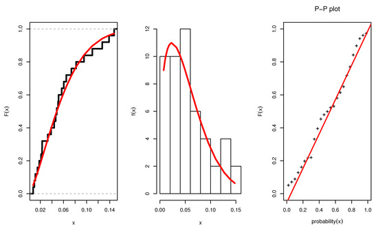
Figure 3. Estimated pdf, CDF, and P-P plots of UEP for the recovery rate of COVID-19 data from Turkey.

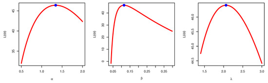
Figure 4. Profile likelihood of UEPD for the recovery rate of COVID-19 data from Turkey.

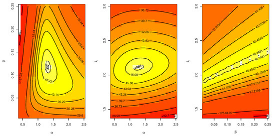
Figure 5. Contour plot of UEP for the recovery rate of COVID-19 data from Turkey.

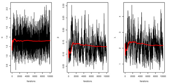
Figure 6. Trace plot of MCMC results for parameters of UEP for the recovery rate of COVID-19 data from Turkey.

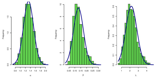
Figure 7. Density plot of posterior MCMC results for parameters of UEP for the recovery rate of COVID-19 data from Turkey.

7.2. Milk Production Data

This data set consists of the total milk output from the first calves of 107 SINDI race cows. The information is available in [52]. In particular, the data set is included in Table 7.

Table 7. Milk production data.

0.0168	0.1546	0.3188	0.3751	0.4332	0.4612	0.515	0.5553	0.6012	0.6768	0.7471
0.0609	0.216	0.3259	0.3821	0.4365	0.4675	0.5232	0.5627	0.6058	0.6789	0.7629
0.065	0.2303	0.3323	0.3891	0.4371	0.4694	0.5285	0.5629	0.6114	0.6844	0.7687
0.0671	0.2356	0.3383	0.3906	0.4438	0.4741	0.5349	0.5707	0.6174	0.686	0.7804
0.0776	0.2361	0.3406	0.3945	0.447	0.4752	0.535	0.5744	0.6196	0.6891	0.8147
0.0854	0.2605	0.3413	0.4049	0.4517	0.48	0.5394	0.577	0.622	0.6907	0.8492
0.1131	0.2681	0.348	0.4111	0.453	0.4823	0.5447	0.5853	0.6465	0.6927	0.8781
0.1167	0.2747	0.3598	0.4143	0.4553	0.499	0.5481	0.5878	0.6488	0.7131
0.1479	0.3134	0.3627	0.4151	0.4564	0.5113	0.5483	0.5912	0.6707	0.7261
0.1525	0.3175	0.3635	0.426	0.4576	0.514	0.5529	0.5941	0.675	0.729

The $M_{L}E$s estimation of the parameters and some measures of goodness of fit were obtained and are displayed in Table 8. It is realized that the minimum values of the goodness-of-fit measures are achieved when using the UEPD, which indicates its superiority and efficiency for modeling the milk production data. The UEPD is compared with eight other suggested models. Figure 8 displays the empirical and fitted CDF, histogram with fitted pdf, and P-P plot of the UEPD model. The profile log probability and the contour plot of the estimated parameters are displayed in Figure 9 and Figure 10. They demonstrate the existence and uniqueness of the MLE.

Table 8. $M_{L}E$ and SE with different measures of goodness of fit for milk production data.

Models	Estimates and SE	$\mathit{\alpha }$	$\mathit{\beta }$	$\mathit{\lambda }$	$\mathit{\theta }$	KS	PVKS	CVM	AD
UEPD	estimates	1.2087	1.1238	0.8427		0.0787	0.5213	0.1088	0.6520
	SE	0.0867	1.0180	0.4151
UW	estimates	0.9846	1.5619			0.1206	0.0890	0.3963	2.4244
	SE	0.1015	0.1064
Kumaraswamy	estimates	2.1949	3.4366			0.0796	0.5162	0.1561	1.0090
	SE	0.2224	0.5821
Beta	estimates	2.4125	2.8297			0.0910	0.3384	0.2083	1.3263
	SE	0.3145	0.3744
KK	estimates	0.3781	5.1808	3.8954	1.4834	0.0790	0.5165	0.1120	0.7195
	SE	0.2337	3.9516	9.2215	2.8696
UG	estimates	2.1191	0.3878			0.1835	0.0015	0.5206	3.0947
	SE	0.8684	0.1145
MOETL	estimates	1.0535	2.0230			0.0968	0.2682	0.2246	1.4262
	SE	0.3475	0.4118
UGG	estimates	4.1576	5.2380	0.4268		0.1067	0.1747	0.2195	1.4377
	SE	1.0592	1.6032	0.1393
EPD	estimates	2.6012	0.6366	1.6623		0.0832	0.4487	0.2318	1.5235
	SE	0.2098	6.2038	42.1400

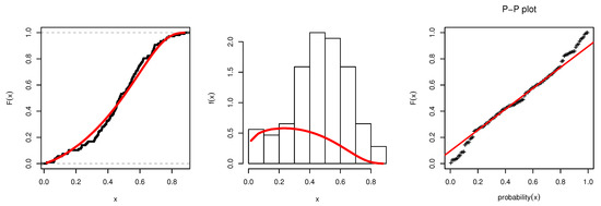
Figure 8. Estimated pdf, CDF, and P-P plots of UEPD for milk production data.

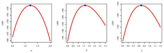
Figure 9. Profile likelihood of UEPD for the milk production data.

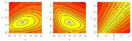
Figure 10. Contour plot of UEPD for the milk production data.

Table 9, summarizes the values of the $M_{L}E$, $MP{S}_p$, and the Bayesian estimates for the UEPD’s parameters. It is noted that the estimated values for each parameter are relatively close when using any method of estimation. This reveals the consistency in our simulated analysis. The $95\%$ asymptotic CONIs and CRIs for the parameters are also computed and the interval lengths show that its shortest length is when using the Bayesian CRI. Figure 11 displays the trace plot of MCMC results for parameters of UEPD for the milk production data, which shows the convergence for these results. Figure 12 displays the density plot of posterior MCMC results for parameters of UEPD for the milk production data, to check the normality plot for these results.

Table 9. $M_{L}E$, $MP{S}_p$, Bayesian estimation methods for milk production data.

Methods		Estimates	SE	Lower	Upper
MLE	$\alpha$	1.2087	0.0867	1.0362	1.3812
	$\beta$	1.1238	1.0180	1.0180	1.2296
	$\lambda$	0.8427	0.4151	0.0290	1.6564
MPS	$\alpha$	1.1531	0.5736	0.0289	2.2772
	$\beta$	1.1827	0.7048	0.0269	2.5642
	$\lambda$	0.8923	0.3892	0.1294	1.6552
Bayesian	$\alpha$	1.2113	0.0791	0.9851	1.4410
	$\beta$	1.2587	0.3279	0.6771	1.8810
	$\lambda$	0.9900	0.3545	0.3666	1.6193

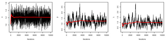
Figure 11. Trace plot of MCMC results for parameters of UEPD for the milk production data.

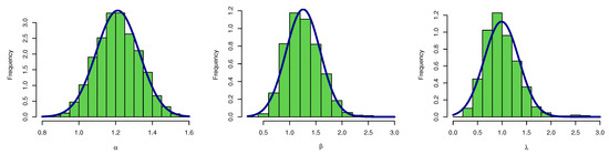
Figure 12. Density plot of posterior MCMC results for parameters of UEPD for the milk production data.

7.3. The Failure Components Data

In this subsection, a real data set is considered from Nigm et al. [53] regarding the ordered failure of 20 components. The data is given in Table 10.

Table 10. Failures of 20 components data.

0.0009	0.004	0.0142	0.0221	0.0261	0.0418	0.0473
0.0834	0.1091	0.1252	0.1404	0.1498	0.175	0.2031
0.2099	0.2168	0.2918	0.3465	0.4035	0.6143

The $M_{L}E$s estimation of the parameters and the goodness-of-fit measures were obtained and are displayed in Table 11. It is realized from Table 11 that the minimum values of the goodness-of-fit measures are achieved when using the UEPD, which indicates its superiority and efficiency for modeling the failure time of components with respect to the six other suggested models. From Table 12, note that the values of the $M_{L}E$, $MP{S}_p$ and Bayesian estimates are close together, which reveals a consistency in our simulated analysis; the $95\%$ asymptotic CONIs and CRIs for the parameters were also computed. Figure 13 displays the empirical and fitted CDF, histogram with fitted pdf, and P-P plot of the UEPD model. The profile log probability and the contour plot of the estimated parameters are displayed in Figure 14 and Figure 15. They demonstrate the existence and uniqueness of the MLE. Figure 16 displays a trace plot of MCMC results for parameters of UEPD for the failure of 20 components data to check convergence for these results. Figure 17 displays the density plot of posterior MCMC results for parameters of UEPD for the failures of 20 components data to check the normality plot for these results.

Table 11. $M_{L}E$ and SE with different measures of goodness of fit for the failure of 20 components data.

Models	Estimates and SE	$\mathit{\alpha }$	$\mathit{\beta }$	$\mathit{\lambda }$	CVMS	ADS	KSD	PVKS
UEPD	estimates	0.7289	0.3755	1.5363	0.0265	0.1649	0.0928	0.9887
	SE	0.1272	0.4975	1.7629
UW	estimates	0.1598	1.7271		0.0567	0.3302	0.1319	0.8334
	SE	0.0710	0.2875
Kumaraswamy	estimates	0.7641	3.4347		0.0290	0.1692	0.1026	0.9700
	SE	0.1752	1.3117
UG	estimates	0.7718	0.5964		0.0912	0.5520	0.1491	0.7110
	SE	0.2786	0.1202
TL	estimates	0.5112			0.0301	0.1754	0.1848	0.4482
	SE	0.1143
MOTL	estimates	0.3520	0.8346		0.0492	0.2785	0.1096	0.9485
	SE	0.2539	0.2739
UGG	estimates	1.3430	3.8518	0.4346	0.0401	0.2268	0.1571	0.6507
	SE	1.0710	2.3086	0.4485
EPD	estimates	0.8999	0.2647	1.6266	0.0428	0.2423	0.1193	0.9067
	SE	0.1654	0.7591	0.4333

Table 12. $M_{L}E$, $MP{S}_p$, Bayesian estimation methods for failures of 20 components data.

Methods		Estimates	SE	Lower	Upper
$M_{L}E$	$\alpha$	0.7289	0.1272	0.4796	0.9782
	$\beta$	0.3755	0.4975	0.2696	0.4813
	$\lambda$	1.5363	1.7629	0.3198	3.3923
$MP{S}_p$	$\alpha$	0.6238	0.1530	0.3239	0.9237
	$\beta$	0.4484	0.2066	0.0435	0.8532
	$\lambda$	1.5716	0.7804	0.0420	3.1011
Bayesian	$\alpha$	0.7473	0.1613	0.4432	1.0613
	$\beta$	0.4126	0.1197	0.1977	0.6520
	$\lambda$	1.6112	0.4591	0.8273	2.5929

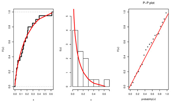
Figure 13. Estimated pdf, CDF, and P-P plots of UEPD for failure of 20 components data.

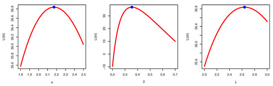
Figure 14. Profile likelihood of UEPD for the failures of 20 components data.

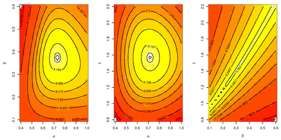
Figure 15. Contour plot of UEPD for the failures of 20 components data.

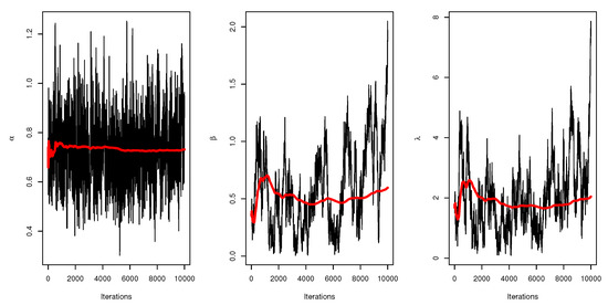
Figure 16. Trace plot of MCMC results for parameters of UEPD for the failures of 20 components data.

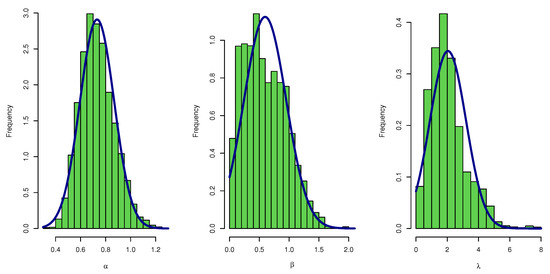
Figure 17. Density plot of posterior MCMC results for parameters of UEPD for the failures of 20 components data.

7.4. Recovery Rate of COVID-19 in France

The WHO confirmed that the first death from COVID-19 in France occurred on 17 March 2020, with the first official recoveries from the pandemic virus occurring on 26 March 2020. From 1 January to 7 February 2022, this data set contains 38 observations calculated as the daily ratio of total recoveries to the cumulative number of confirmed cases and different cumulative numbers of confirmed death cases in France, see Table 13. Accessed by https://en.wikipedia.org/wiki/COVID-19_pandemic_in_France).

Table 13. Recovery rate of COVID-19 Data in France.

0.195	0.2338	0.2368	0.1073	0.1592	0.2784	0.0689	0.1791
0.1121	0.1865	0.2631	0.0716	0.1411	0.1477	0.1874	0.0853
0.0922	0.1711	0.1962	0.2146	0.1041	0.1524	0.1811	0.0643
0.2698	0.1245	0.176	0.2363	0.0712	0.1361	0.1386
0.3316	0.077	0.1367	0.1549	0.2178	0.0951	0.1346

From Table 14, it is clear that the UEPD has the minimum goodness-of-fit measure and the maximum PVKS. This reveals the suitability of the UEPD to fit the recovery rate of COVID-19 in France. Table 15 summarizes the values of estimators under MLE, MPS, and Bayesian methods. We can view the close values of estimators for all methods which prove consistency in this simulation. In addition, the $95\%$ asymptotic CONIs and the CRIs for the parameters $\alpha$, $\beta$ and $\lambda$ are computed for the recovery rate of COVID-19 in France.

Table 14. $M_{L}E$ and SE with different measures of goodness of fit for the recovery rate of COVID-19 data in France.

Models	Estimates and SE	$\mathit{\alpha }$	$\mathit{\beta }$	$\mathit{\lambda }$	CVMS	ADS	KSD	PVKS
UEPD	estimates	2.1715	0.3544	2.6397	0.0365	0.2965	0.0722	0.9807
	SE	0.2651	0.1115	0.5027
UW	estimates	0.0280	4.8690		0.0844	0.5464	0.1203	0.5994
	SE	0.0145	0.5965
MOK	estimates	0.1490	3.8135	191.1284	0.1700	1.0407	0.1542	0.2952
	SE	0.1142	0.9003	88.8899
UG	estimates	0.0073	2.3191		0.1700	1.0407	0.1542	0.2952
	SE	0.0039	0.2286
MOETL	estimates	0.0042	4.2695		0.0639	0.4531	0.0769	0.9653
	SE	0.0021	0.4101
UGLBXII	estimates	2.0928	3.0810	2.2037	0.0429	0.3210	0.0788	0.9573
	SE	1.2820	1.0797	0.8284
UGG	estimates	2.5233	157.2439	1.3847	0.0631	0.4369	0.1534	0.3010
	SE	0.4258	77.1515	0.7092

Table 15. $M_{L}E$, $MP{S}_p$, Bayesian estimation methods for pandemic coronavirus in France data.

Method		Estimates	SE	Lower	Upper
MLE	$\alpha$	2.1715	0.2651	1.9222	2.4209
	$\beta$	0.3544	0.1115	0.2486	0.4603
	$\lambda$	2.6397	0.5027	0.7837	4.4957
MPS	$\alpha$	2.0015	0.9577	0.1244	3.8786
	$\beta$	0.3849	0.1267	0.1366	0.6331
	$\lambda$	2.8257	0.5472	1.7531	3.8982
Bayesian	$\alpha$	2.1585	0.2483	1.6877	2.6627
	$\beta$	0.2981	0.1172	0.0673	0.5083
	$\lambda$	1.9924	1.3850	0.0208	4.7526

Figure 18 illustrates the plots of the estimated pdf, CDF, and P-P plots of UEPD for the recovery rate of COVID-19 in France. We plot the profile likelihood in Figure 19, which indicates the uniqueness of the maximum. The contour plot in Figure 20 also shows that the $M_{L}E$ has unique values with maximum log-likelihood. Figure 21 displays the trace plots of the MCMC results for the above data, it shows convergence results. while Figure 22 plots the posterior MCMC for the UEPD parameters to check the normality plot for these results.

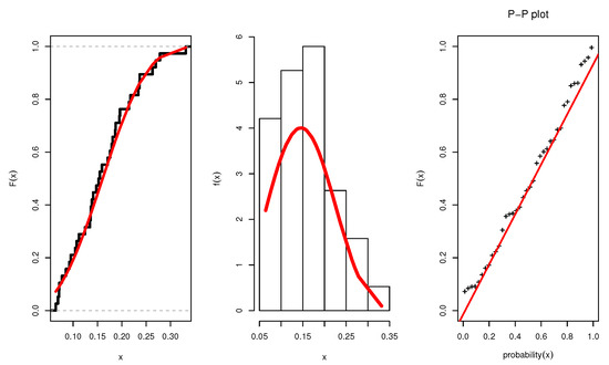
Figure 18. Estimated pdf, CDF and P-P plots of UEPD for France COVID-19 data.

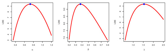
Figure 19. Profile likelihood of UEPD for France COVID-19 data.

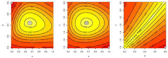
Figure 20. Contour plot of UEPD for France COVID-19 data.

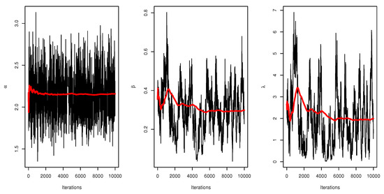
Figure 21. Trace plot of MCMC results for parameters of UEPD for the failure of 20 components data.

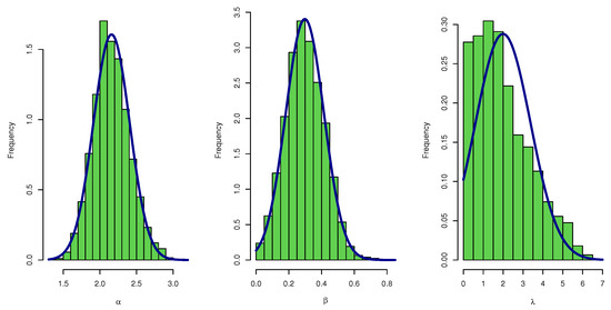
Figure 22. Density plot of posterior MCMC results for parameters of UEPD for the failure of 20 components data.

8. Results of Simulation

Simulation research was carried out to evaluate the interpretation of the estimating techniques discussed previously. The following procedure was used to assess the efficiency of the estimators:

First step: Generate a random sample with size n from the UEPD.

Second step: The results of the first step are utilized to calculate the $\widehat{\theta }=\left(\widehat{\alpha },\widehat{\beta },\widehat{\lambda }\right)$ considering the $M_{L}E$, $MP{S}_p$ and Bayesian estimators.

Third step: Repeat the first and second steps N times.

Fourth step: Using $\widehat{\theta }=\left(\widehat{\alpha },\widehat{\beta },\widehat{\lambda }\right)$and $\theta =\left(\alpha ,\beta ,\lambda \right)$, calculate the bias and the average squared error (AVSE).

The numerical results were calculated using the $nlminb$ function (in the stat package) and Nelder–Mead approach in R software. From the UEPD, 5000 samples were generated, where $n=(50;100;150)$, and by choosing starting values ${\alpha }_{\circ }$$=0.60$, ${\beta }_{\circ }=0.04$ and ${\lambda }_{\circ }$ $=0.0$, the comparisons of the different approaches of the estimators of $\alpha ,\beta$ and $\lambda ,$ were considered regarding the AVSE, which is calculated for $k=1,2,3,$$({\theta }_1=\alpha ,{\theta }_2=\beta ,{\theta }_3=\lambda )$, as $AVSE\left({\theta }_k\right)=\frac{1}{M}\sum _{i=1}^M{\left({\widehat{\theta }}_k^{\left(i\right)}-{\theta }_k\right)}^2,$ where $M=5000$ is the number of simulated samples.

Another criterion was also applied for comparing the 95% CONIs; this is achieved using asymptotic distributions of the $M_{L}E$s and the $MP{S}_p$ with the idea of CRIs. They are compared in view of the average confidence interval lengths (ACLs). The hyper-parameters in the case of informative priors are chosen as follows: $a_1=a_2=2,a_3=5$,$b_1=4,b_2=3$ and $b_3=6$, while in case of non-informative priors, the values of $a_j,b_j,$, where $j=1,2,3$, were chosen to be equal to zero.

All estimates illustrate the consistency property, which means the AVSEs decrease as the sample size increases for all parameter values. It is shown that the AVSEs illustrate that the $MP{S}_p$ estimation method outperforms all other estimators for all parameter combinations.

Table 16 and Table 17 show the outcomes of the estimated parameters and their AVSE, as well as the asymptotic and credible intervals.

Table 16. $M_{L}E$, $MP{S}_p$ and Bayesian estimation methods for parameters of UEPD for $\beta =0.5$.

$\mathit{\beta }=0.5$				${\mathit{M}}_{\mathit{L}}\mathit{E}$			${\mathbf{MPS}}_{\mathit{p}}$			Bayesian
$\mathit{\beta }$	$\mathit{\lambda }$	n		Bias	AVSE	L.CI	Bias	AVSE	L.CI	Bias	AVSE	L.CI
0.5	0.6	30	$\alpha$	0.0776	0.0133	0.3347	0.0245	0.0064	0.2993	0.0285	0.0059	0.2787
			$\beta$	0.0338	0.0053	0.2518	0.0243	0.0031	0.1958	0.0096	0.0049	0.2354
			$\lambda$	0.0595	0.0128	0.3768	−0.0429	0.0094	0.3399	0.0170	0.0099	0.3707
		80	$\alpha$	0.0583	0.0054	0.1738	0.0337	0.0029	0.1651	0.0235	0.0023	0.1611
			$\beta$	0.0425	0.0036	0.1640	0.0297	0.0018	0.1185	0.0132	0.0035	0.1428
			$\lambda$	0.0542	0.0061	0.2191	−0.0510	0.0054	0.2056	0.0153	0.0049	0.2672
		150	$\alpha$	0.0559	0.0042	0.1284	0.0409	0.0027	0.1245	0.0187	0.0013	0.1189
			$\beta$	0.0427	0.0031	0.1376	0.0315	0.0016	0.0940	0.0041	0.0023	0.1858
			$\lambda$	0.0529	0.0046	0.1672	−0.0528	0.0044	0.1596	0.0135	0.0021	0.1634
	2.4	30	$\alpha$	0.0763	0.0122	0.3123	0.0363	0.0057	0.2799	0.0392	0.0063	0.2646
			$\beta$	0.0222	0.0235	0.5955	0.0833	0.0392	0.7041	0.0049	0.0077	0.3312
			$\lambda$	0.0676	0.0260	0.5744	−0.0449	0.0099	0.3483	0.0058	0.0159	0.4865
		80	$\alpha$	0.0599	0.0057	0.1799	0.0354	0.0031	0.1707	0.0369	0.0033	0.1749
			$\beta$	0.0257	0.0101	0.3805	0.0352	0.0135	0.4350	0.0019	0.0048	0.2683
			$\lambda$	0.0863	0.0181	0.4044	−0.0176	0.0026	0.1866	0.0063	0.0069	0.3350
		150	$\alpha$	0.0550	0.0041	0.1293	0.0340	0.0026	0.1254	0.0293	0.0018	0.1179
			$\beta$	0.0298	0.0057	0.2722	0.0209	0.0064	0.3033	0.0035	0.0022	0.1819
			$\lambda$	0.0897	0.0143	0.3112	−0.0103	0.0011	0.1256	0.0018	0.0027	0.2055
2	0.6	30	$\alpha$	0.3055	0.1881	1.2074	0.1922	0.0832	1.0718	0.0110	0.0154	0.4680
			$\beta$	0.0247	0.0033	0.2047	0.0924	0.0025	0.1704	0.0129	0.0032	0.2004
			$\lambda$	0.0216	0.0141	0.4587	−0.0391	0.0004	0.0724	0.0044	0.0121	0.4076
		80	$\alpha$	0.2373	0.0863	0.6787	0.1848	0.0459	0.6412	0.0135	0.0061	0.2985
			$\beta$	0.0269	0.0017	0.1223	0.0271	0.0014	0.1011	0.0092	0.0016	0.1169
			$\lambda$	0.0181	0.0051	0.2716	−0.0108	0.0002	0.0428	0.0082	0.0046	0.2531
		150	$\alpha$	0.2220	0.0667	0.5178	0.1613	0.0422	0.4987	0.0107	0.0028	0.2038
			$\beta$	0.0263	0.0011	0.0780	0.0272	0.0011	0.0754	0.0077	0.0008	0.1099
			$\lambda$	0.0174	0.0029	0.1982	−0.0108	0.0002	0.0317	0.0062	0.0025	0.1904
	2.4	30	$\alpha$	0.3057	0.1908	1.2240	0.0922	0.0843	1.0799	0.0098	0.0148	0.4700
			$\beta$	0.0074	0.0021	0.1795	0.0175	0.0028	0.1954	0.0163	0.0020	0.1788
			$\lambda$	0.0091	0.0397	0.7803	−0.0018	0.0000	0.0206	0.0052	0.0143	0.4714
		80	$\alpha$	0.2302	0.0835	0.6854	0.0813	0.0449	0.6496	0.0095	0.0075	0.3238
			$\beta$	0.0007	0.0007	0.1072	0.0093	0.0010	0.1189	0.0119	0.0005	0.0912
			$\lambda$	0.0142	0.0114	0.4159	−0.0009	0.0000	0.0125	0.0029	0.0071	0.3150
		150	$\alpha$	0.2164	0.0630	0.4985	0.0816	0.0395	0.4831	0.0091	0.0026	0.1930
			$\beta$	0.0001	0.0004	0.0760	0.0052	0.0005	0.0823	0.0085	0.0004	0.0759
			$\lambda$	0.0174	0.0066	0.3124	−0.0004	0.0000	0.0086	0.0019	0.0028	0.2043

Table 17. $M_{L}E$, $MP{S}_p$ and Bayesian estimation methods for parameters of UEPD when $\beta =2$.

$\mathit{\beta }=2$				${\mathit{M}}_{\mathit{L}}\mathit{E}$			${\mathbf{MPS}}_{\mathit{p}}$			Bayesian
$\mathit{\beta }$	$\mathit{\lambda }$	n		Bias	AVSE	L.CI	Bias	AVSE	L.CI	Bias	AVSE	L.CI
0.5	0.6	30	$\alpha$	0.0776	0.0133	0.3347	0.0409	0.0064	0.2993	0.0285	0.0059	0.2787
			$\beta$	0.0338	0.0053	0.2518	0.0315	0.0031	0.1958	0.0096	0.0049	0.2354
			$\lambda$	0.0595	0.0128	0.3768	−0.0528	0.0094	0.3399	0.0170	0.0099	0.3707
		80	$\alpha$	0.0583	0.0054	0.1738	0.0337	0.0029	0.1651	0.0235	0.0023	0.1611
			$\beta$	0.0425	0.0036	0.1640	0.0297	0.0018	0.1185	0.0091	0.0035	0.1528
			$\lambda$	0.0542	0.0061	0.2191	−0.0510	0.0054	0.2056	0.0153	0.0049	0.2672
		150	$\alpha$	0.0559	0.0042	0.1284	0.0245	0.0027	0.1245	0.0187	0.0013	0.1189
			$\beta$	0.0427	0.0031	0.1376	0.0243	0.0016	0.0940	0.0041	0.0023	0.1486
			$\lambda$	0.0529	0.0046	0.1672	−0.0429	0.0044	0.1596	0.0135	0.0021	0.1634
	2.4	30	$\alpha$	0.0763	0.0122	0.3123	0.0424	0.0057	0.2799	0.0392	0.0063	0.2646
			$\beta$	0.0222	0.0235	0.5955	0.0833	0.0392	0.7041	0.0049	0.0077	0.3312
			$\lambda$	0.0676	0.0260	0.5744	−0.0449	0.0099	0.3483	0.0066	0.0159	0.4865
		80	$\alpha$	0.0599	0.0057	0.1799	0.0414	0.0031	0.1707	0.0369	0.0033	0.1749
			$\beta$	0.0257	0.0101	0.3805	0.0352	0.0135	0.4350	0.0042	0.0048	0.2683
			$\lambda$	0.0863	0.0181	0.4044	−0.0176	0.0026	0.1866	0.0063	0.0069	0.3350
		150	$\alpha$	0.0550	0.0041	0.1293	0.0401	0.0026	0.1254	0.0293	0.0018	0.1179
			$\beta$	0.0298	0.0057	0.2722	0.0209	0.0064	0.3033	0.0035	0.0022	0.1819
			$\lambda$	0.0897	0.0143	0.3112	−0.0103	0.0011	0.1256	0.0018	0.0027	0.2055
2	0.6	30	$\alpha$	0.0751	0.0123	0.3204	0.0400	0.0058	0.2855	0.0284	0.0055	0.2557
			$\beta$	0.1086	0.0257	0.4621	0.0106	0.0003	0.0665	0.0006	0.0093	0.3750
			$\lambda$	0.0569	0.0158	0.4393	−0.0707	0.0150	0.4395	0.0167	0.0087	0.3506
		80	$\alpha$	0.0616	0.0060	0.1822	0.0370	0.0033	0.1732	0.0273	0.0026	0.1651
			$\beta$	0.1259	0.0241	0.3559	0.0099	0.0002	0.0413	0.0012	0.0061	0.2933
			$\lambda$	0.0610	0.0083	0.2662	−0.0667	0.0094	0.2761	0.0188	0.0051	0.2646
		150	$\alpha$	0.0549	0.0041	0.1271	0.0224	0.0026	0.1233	0.0196	0.0012	0.1125
			$\beta$	0.1335	0.0244	0.3190	0.0070	0.0002	0.0291	0.0002	0.0026	0.2020
			$\lambda$	0.0600	0.0058	0.1855	−0.0495	0.0075	0.1963	0.0158	0.0022	0.1754
	2.4	30	$\alpha$	0.0792	0.0129	0.3181	0.0262	0.0060	0.2848	0.0374	0.0062	0.2586
			$\beta$	0.0378	0.1281	1.3957	0.0375	0.0491	0.8566	0.0048	0.0102	0.3813
			$\lambda$	0.0566	0.0816	1.0984	−0.1018	0.1248	1.3268	0.0020	0.0141	0.4586
		80	$\alpha$	0.0579	0.0053	0.1754	0.0333	0.0029	0.1665	0.0372	0.0034	0.1757
			$\beta$	0.0213	0.0513	0.8842	0.0247	0.0187	0.5276	0.0028	0.0058	0.2932
			$\lambda$	0.0482	0.0335	0.6920	−0.0547	0.0480	0.8318	0.0001	0.0067	0.3178
		150	$\alpha$	0.0551	0.0041	0.1291	0.0402	0.0026	0.1255	0.0290	0.0018	0.1203
			$\beta$	0.0411	0.0297	0.6561	0.0202	0.0099	0.3819	0.0030	0.0025	0.1934
			$\lambda$	0.0389	0.0169	0.4867	−0.0394	0.0243	0.5916	0.0001	0.0029	0.2091

• The findings of Table 16 and Table 17 show that the UEPD is stable because the range of biases, AVSEs, and CI lengths for all the parameters is quite narrow.
• In some instances, we notice that as the sample size grows larger, the AVSEs for all estimations decrease.
• This shows that various estimation techniques have good results for big sample sizes in terms of bias and AVSEs.
• $MP{S}_p$ Estimation methods has better measures than the $M_{L}E$ method.
• The Bayesian estimation method is the best estimation method to estimate the parameter of UEPD.
• The results of the simulation revealed empirical proof of the stability of our estimates.

9. Conclusions

In this paper, we introduced the unit exponential Pareto distribution to model real data examples from the recovery rate of COVID-19 during the pandemic, in addition to other applications from different fields. The unit exponential Pareto distribution is a powerful tool for modeling extreme values in a population and understanding the underlying patterns and trends in the data. It can provide valuable insights into the characteristics of the data and help to make good decisions. Consequently, many important characteristics were studied, such as the shape of the density and hazard rate functions; the $Q{U}_{N}F$, $M_O$s, $M_{O}GF$; five different types of entropy such as RE, HCE, TE, AE and MHE; and $O_S$, $S_S$ and $S_{OR}$ were obtained. The unknown parameters were estimated using the $M_L$ method, the $MP{S}_P$, and the Bayesian estimations, and their performances were compared using simulation experiments. In general, it was observed that the $MP{S}_P$s estimation outperforms the other methods; hence, for small sample sizes, the $MP{S}_P$ estimators have a lower mean squared error than the others. We used three goodness-of-fit criteria to prove the benefit of the proposed UEPD for modeling real skewed data sets. A simulation was carried out to examine the parameters’ bias, average square error, and confidence interval lengths. Based on observed results, one can use this model to describe other features related to biomedical, mechanical, and economical fields.

References

- Tregoning, J.S.; Brown, E.S.; Cheeseman, H.M.; Flight, K.E.; Higham, S.L.; Lemm, N.M.; Pierce, B.F.; Stirling, D.C.; Wang, Z.; Pollock, K.M. Vaccines for COVID-19. Clin. Exp. Immunol. 2020, 202, 162–192. [Google Scholar] [CrossRef] [PubMed]
- Sun, H.T.; Luu, A.M.B.Q.; Widdicombe, J.; Ashammakhi, N.; Li, S. Recent advances in vitro lung microphysiological systems for Covid-19 modeling and drug development. Curr. Med. Chem. 2020. [Google Scholar]
- Provder, T. Computer Applications in Applied Polymer Science II. In American Chemical Society; Chemical Congress of North America: Toronto, ON, USA, 1989; ISBN13: 9780841216624. [Google Scholar] [CrossRef]
- Johnson, N.L. Systems of frequency curves generated by methods of translation. Biometrika 1949, 36, 149–176. [Google Scholar] [CrossRef] [PubMed]
- Kumaraswamy, P. A generalized probability density function for double-bounded random processes. J. Hydrol. 1980, 46, 79–88. [Google Scholar] [CrossRef]
- Mazucheli, J.; Menezes, A.F.B.; Ghitany, M.E. The unit-Weibull distribution and associated inference. J. Appl. Probab. Stat. 2018, 13, 1–22. [Google Scholar]
- Mazucheli, J.; Menezes, A.F.B.; Fernandes, L.B.; de Oliveira, R.P.; Ghitany, M.E. The unit-Weibull distribution as an alternative to the Kumaraswamy distribution for the modeling of quantiles conditional on covariates. J. Appl. Stat. 2020, 47, 954–974. [Google Scholar] [CrossRef]
- Mazucheli, J.; Menezes, A.F.; Dey, S. Unit-Gompertz distribution with applications. Statistica 2019, 79, 25–43. [Google Scholar]
- Mazucheli, J.; Menezes, A.F.; Dey, S. The unit-Birnbaum–Saunders distribution with applications. Chil. J. Stat. 2018, 9, 47–57. [Google Scholar]
- Ghitany, M.E.; Mazucheli, J.; Menezes, A.F.B.; Alqallaf, F. The unit-inverse Gaussian distribution: A new alternative to two-parameter distributions on the unit interval. Commun. Stat. Theory Methods 2019, 48, 3423–3438. [Google Scholar] [CrossRef]
- Korkmaz, M.Ç. The unit generalized half normal distribution: A new bounded distribution with inference and application. Univ. Politeh. Buchar. Sci. Bull. Ser. A Appl. Math. Phys. 2020, 82, 133–140. [Google Scholar]
- Bantan, R.A.R.; Chesneau, C.; Jamal, F.; Elgarhy, M.; Tahir, M.H.; Ali, A.; Zubair, M.; Anam, S. Some New Facts about the Unit-Rayleigh Distribution with Applications. Mathematics 2020, 8, 1954. [Google Scholar] [CrossRef]
- Korkmaz, M.Ç.; Chesneau, C. On the unit Burr-XII distribution with the quantile regression modeling and applications. Comp. Appl. Math. 2021, 40. [Google Scholar] [CrossRef]
- Korkmaz, M.Ç.; Emrah, A.; Chesneau, C.; Yousof, H.M. On the Unit-Chen distribution with associated quantile regression and applications. Math. Slovaca 2022, 72, 765–786. [Google Scholar] [CrossRef]
- Bantan, R.A.R.; Shafiq, S.; Tahir, M.H.; Elhassanein, A.; Jamal, F.; Almutiry, W.; Elgarhy, M. Statistical Analysis of COVID-19 Data: Using A New Univariate and Bivariate Statistical Model. J. Funct. Spaces 2022, 2022. [Google Scholar] [CrossRef]
- Arnold, B.C. Pareto Distributions; International Cooperative Publishing House: Fairland, MA, USA, 1983. [Google Scholar]
- Alzaatreh, A.; Famoye, F.; Lee, C. Weibull-Pareto distribution and its applications. Commun. Stat.-Theory Methods 2013, 42, 1673–1691. [Google Scholar] [CrossRef]
- Alzaatreh, A.; Ghosh, I. A study of the Gamma-Pareto (IV) distribution and its applications. Commun. Stat.-Theory Methods 2016, 45, 636–654. [Google Scholar] [CrossRef]
- Akinsete, A.; Famoye, F.; Lee, C. The beta-Pareto distribution. Statistics 2008, 42, 547–563. [Google Scholar] [CrossRef]
- Mahmoudi, E. The beta generalized Pareto distribution with application to lifetime data. Math. Comput. Simul. 2011, 81, 2414–2430. [Google Scholar] [CrossRef]
- Elbatal, I. The Kumaraswamy exponentiated Pareto distribution. Econ. Qual. Control 2013, 28, 1–8. [Google Scholar] [CrossRef]
- Tahir, M.H.; Cordeiro, G.M.; Mansoor, M.; Zubair, M. The Weibull-Lomax distribution: Properties and applications. Hacet. J. Math. Stat. 2015, 44, 455–474. [Google Scholar] [CrossRef]
- Bdair, O.; Ahmad, H.H. Estimation of The Marshall-Olkin Pareto Distribution Parameters: Comparative Study. Rev. Investig. Oper. 2021, 42, 440–455. [Google Scholar]
- Haj Ahmad, H.H.; Almetwally, E. Marshall-Olkin Generalized Pareto Distribution: Bayesian and Non Bayesian Estimation. Pak. J. Stat. Oper. Res. 2020, 16, 21–33. [Google Scholar] [CrossRef]
- Almetwally, E.; Ahmad, H.H. A New Generalization of Pareto Distribution with Applications. Statistics in Transition NewSeries 2020, 21, 61–84. [Google Scholar] [CrossRef]
- Almetwally, E.; Ahmad, H.H.; Almongy, H. Extended Odd Weibull Pareto Distribution, Estimation and Applications. J. Stat. Appl. Probab. 2022, 11, 795–809. [Google Scholar]
- Altun, E.; Cordeiro, G.M. The unit-improved second-degree Lindley distribution: Inference and regression modeling. Comput. Stat. 2020, 35, 259–279. [Google Scholar] [CrossRef]
- Altun, E.; Hamedani, G.G. The log-xgamma distribution with inference and application. J. Soc. Franç. Stat. 2018, 159, 40–55. [Google Scholar]
- Déniz, E.G.; Sordo, M.A.; Ojeda, E.C. The log-Lindley distribution as an alternative to the beta regression model with applications in insurance. Insur. Math. Econ. 2014, 54, 49–57. [Google Scholar] [CrossRef]
- Gündüz, S.; Korkmaz, M.Ç. A new unit distribution based on the unbounded Johnson distribution rule: The unit Johnson SU distribution. Pak. J. Stat. Oper. Res. 2020, 16, 471–490. [Google Scholar] [CrossRef]
- Korkmaz, M.Ç.; Chesneau, C.; Korkmaz, Z.S. Transmuted unit Rayleigh quantile regression model: Alternative to beta and Kumaraswamy quantile regression models. Univ. Politeh. Buchar. Sci. Bull. Ser. A Appl. Math. Phys. 2021; to appear. [Google Scholar]
- Mazucheli, J.; Menezes, A.F.B.; Chakraborty, S. On the one parameter unit-Lindley distribution and its associated regression model for proportion data. J. Appl. Stat. 2019, 46, 700–714. [Google Scholar] [CrossRef]
- Al-Kadim, K.A.; Boshi, M.A. Exponential Pareto distribution. Math. Theory Model. 2013, 3(5), 135–146. [Google Scholar]
- Rényi, A. On measures of entropy and information. In Proceedings of the 4th Fourth Berkeley Symposium on Mathematical Statistics and Probability, Berkeley, CA, USA, 20–30 June 1961; pp. 547–561. [Google Scholar]
- Havrda, J.; Charvat, F. Quantification method of classification processes, Concept of Structural-Entropy. Kybernetika 1967, 3, 30–35. [Google Scholar]
- Tsallis, C. The role of constraints within generalized non-extensive statistics. Physica 1998, 261, 547–561. [Google Scholar]
- Arimoto, S. Information-theoretical considerations on estimation problems. Inf. Control 1971, 19, 181–194. [Google Scholar] [CrossRef]
- Mathai, A.M.; Haubold, H.J. On generalized distributions and pathways. Phys. Lett. A 2008, 372, 2109–2113. [Google Scholar] [CrossRef]
- Surles, J.G.; Padgett, W.J. Inference for reliability and stress-strength for a scaled Burr Type X distribution. Lifetime Data Anal. 2001, 7, 187–200. [Google Scholar] [CrossRef] [PubMed]
- Lawless, J.F. Statistical Models and Methods for Lifetime Data; John Wiley and Sons: New York, NY, USA, 1982. [Google Scholar]
- Khalifa, E.H.; Ramadan, D.A.; El-Desouky, B.S. Statistical Inference of Truncated Weibull-Rayleigh Distribution: Its Properties and Applications. Open J. Model. Simul. 2021, 9, 281–298. [Google Scholar] [CrossRef]
- Buzaridah, M.M.; Ramadan, D.A.; El-Desouky, B.S. Flexible Reduced Logarithmic-Inverse Lomax Distribution with Application for Bladder Cancer. Open J. Model. Simul. 2021, 9, 351–369. [Google Scholar] [CrossRef]
- Cheng, R.C.H.; Amin, N.A.K. Maximum product of spacings estimation with application to the log-normal distribution. Math Rep. 1979, 10, 1–15. [Google Scholar]
- Ranneby, B. The Maximum Spacing Method. An Estimation Method Related to the Maximum Likelihood Method. Scand. J. Stat. 1984, 11, 93–112. [Google Scholar]
- Gupta, A.K.; Nadarajah, S. Handbook of Beta Distribution and Its Applications; CRC Press: Boca Raton, FL, USA, 2004. [Google Scholar]
- El-Sherpieny, E.S.A.; Ahmed, M.A. On the Kumaraswamy Kumaraswamy distribution. Int. J. Basic Appl. Sci. 2014, 3, 372. [Google Scholar] [CrossRef]
- George, R.; Thobias, S. Marshall-Olkin Kumaraswamy distribution. Int. Math.Forum 2017, 12, 47–69. [Google Scholar] [CrossRef]
- Opone, F.C.; Osemwenkhae, J.E. The Transmuted Marshall-Olkin Extended Topp-Leone Distribution. Earthline J. Math. Sci. 2022, 9, 179–199. [Google Scholar] [CrossRef]
- Bhatti, F.A.; Ali, A.; Hamedani, G.; Korkmaz, M.C.; Ahmad, M. The unit generalized log Burr XII distribution: Properties and application. AIMS Math. 2021, 6, 10222–10252. [Google Scholar] [CrossRef]
- Topp, C.W.; Leone, F.C. A Family of J-Shaped Frequency Functions. J. Am. Stat. Assoc. 1955, 50, 209–219. [Google Scholar] [CrossRef]
- Bantan, R.A.; Jamal, F.; Chesneau, C.; Elgarhy, M. Theory and applications of the unit gamma/Gompertz distribution. Mathematics 2021, 9, 1850. [Google Scholar] [CrossRef]
- Cordeiro, G.M.; dos Santos Brito, R. The beta power distribution. Braz. J. Probab. Stat. 2012, 26, 88–112. [Google Scholar]
- Nigm, A.M.; Al-Hussaini, E.K.; Jaheen, Z.F. Bayesian one-sample prediction of future observations under Pareto distribution. Statistics 2003, 37, 527–536. [Google Scholar] [CrossRef]
Disclaimer/Publisher’s Note: The statements, opinions and data contained in all publications are solely those of the individual author(s) and contributor(s) and not of MDPI and/or the editor(s). MDPI and/or the editor(s) disclaim responsibility for any injury to people or property resulting from any ideas, methods, instructions or products referred to in the content. |
© 2023 by the authors. Licensee MDPI, Basel, Switzerland. This article is an open access article distributed under the terms and conditions of the Creative Commons Attribution (CC BY) license (https://creativecommons.org/licenses/by/4.0/).