
Failure Risk Assessment of Coal Gasifier Based on the Integration of Bayesian Network and Trapezoidal Intuitionistic Fuzzy Number-Based Similarity Aggregation Method (TpIFN-SAM)


Abstract
:1. Introduction
2. Preliminaries
2.1. Intuitionistic Fuzzy Set
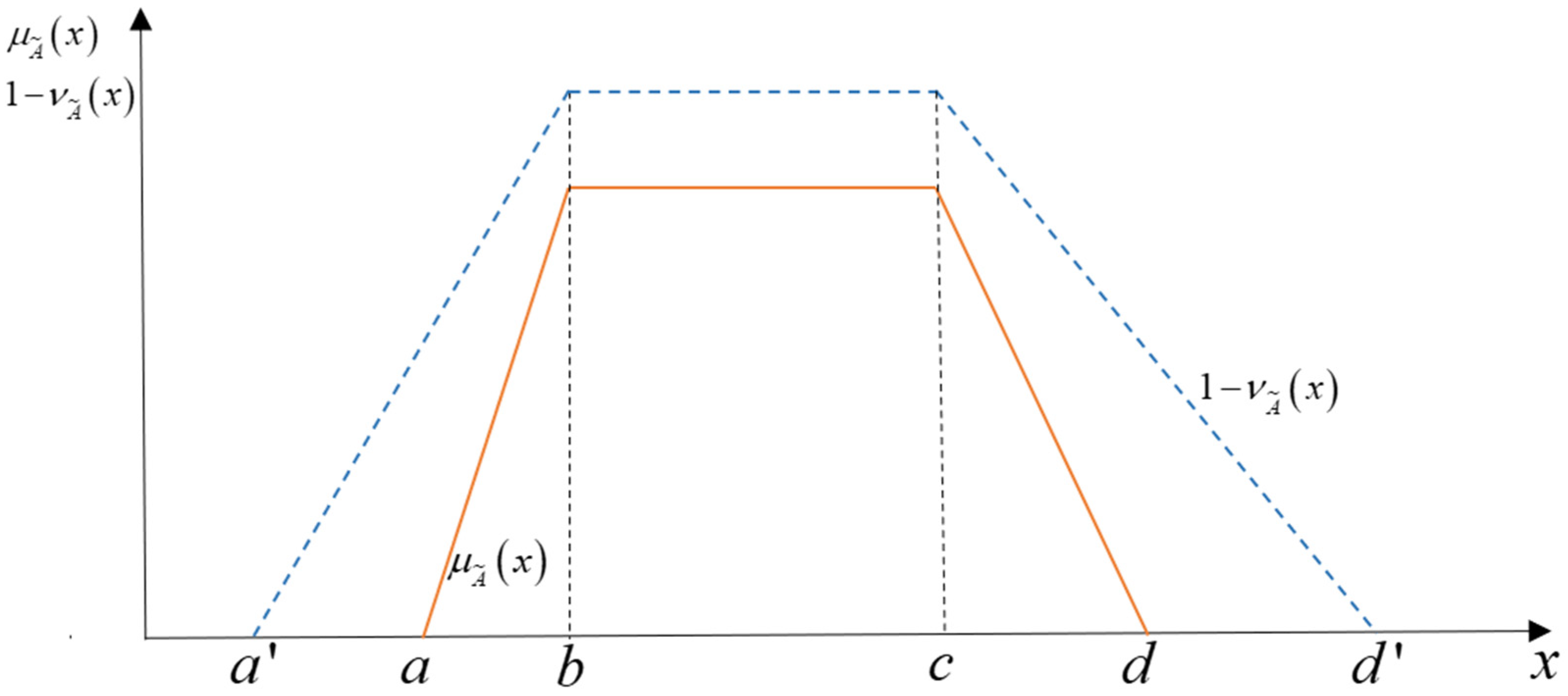
2.2. Trapezoidal Intuitionistic Fuzzy Number
2.3. The Expectation of a TpIFN
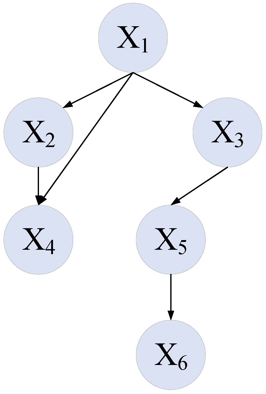
2.4. Bayesian Network
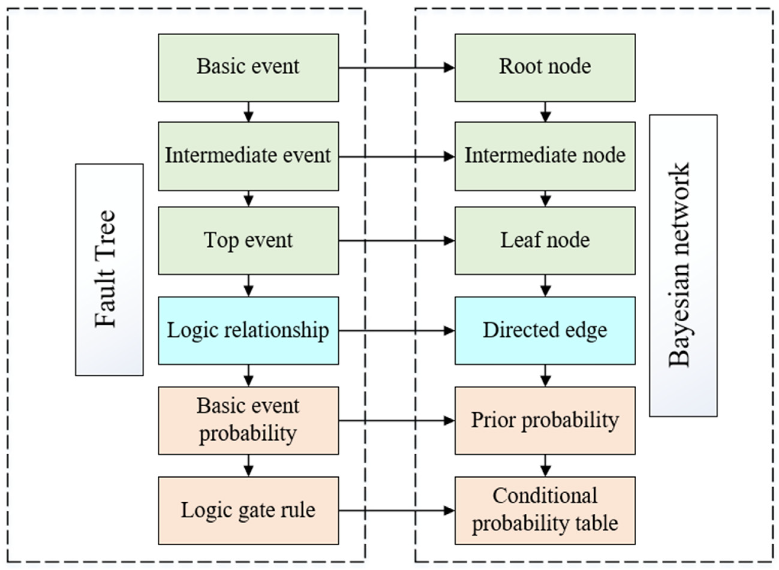
2.5. Mapping to Bayesian Network from Fault Tree
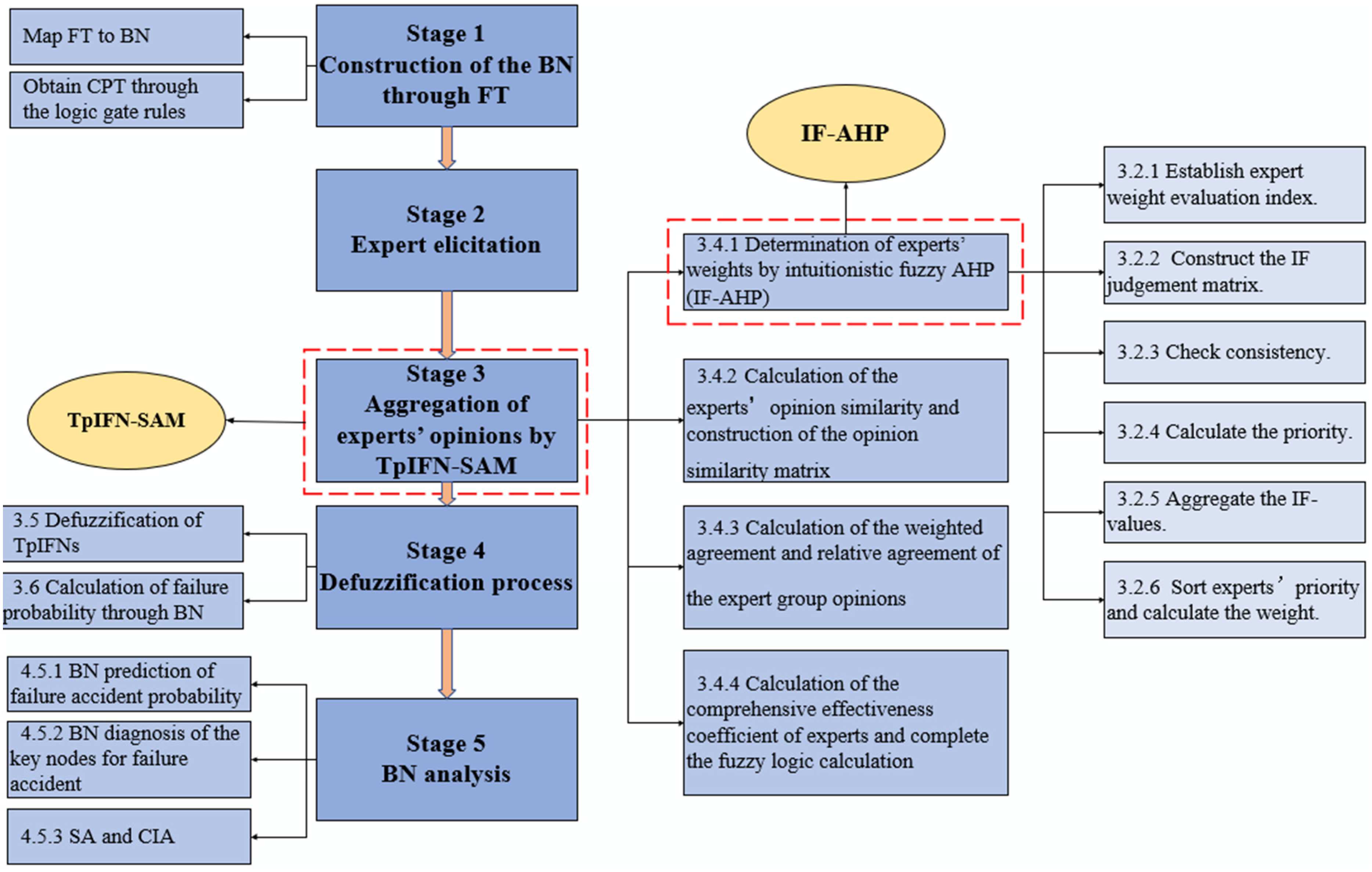
3. Proposed Model for Failure-Risk Assessment Based on BN with TpIFN-SAM
3.1. General Framework
3.2. Construction of the BN through FT
3.3. Expert Elicitation
3.4. Aggregation of Experts’ Opinions by TpIFN-SAM
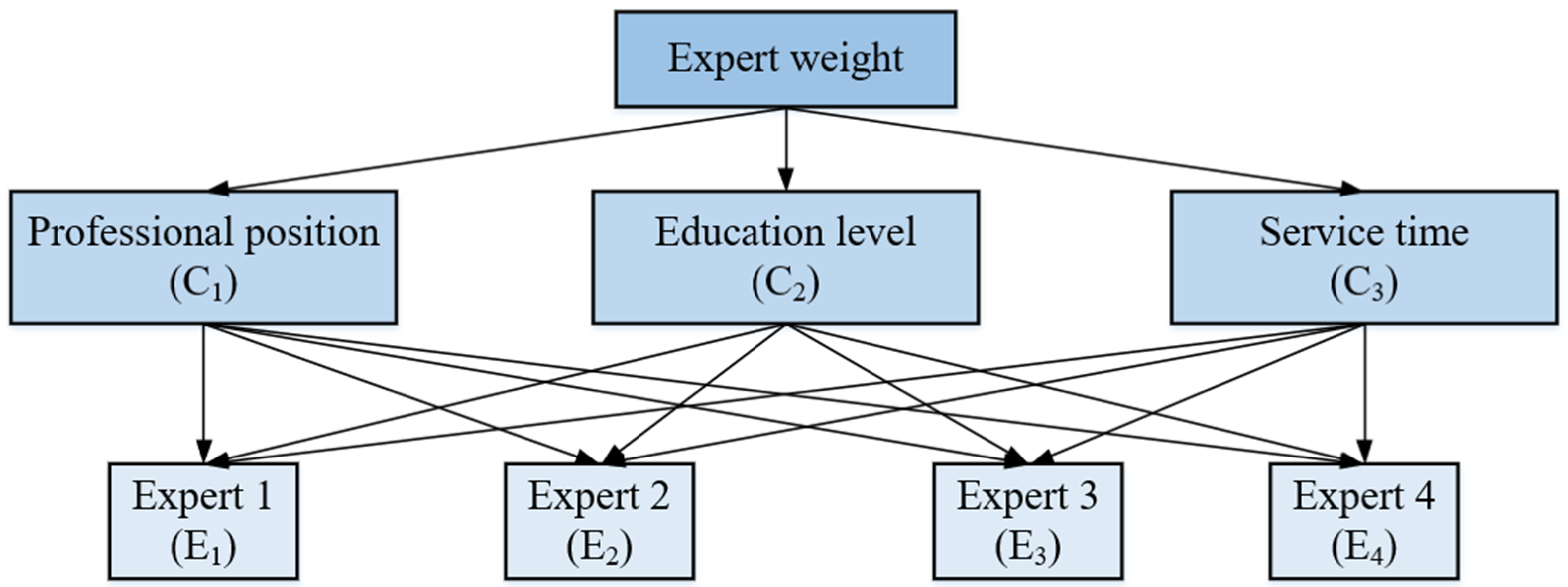
3.4.1. Determination of Experts’ Weights by Intuitionistic Fuzzy AHP (IF-AHP)
3.4.2. Calculation of the Experts’ Opinion Similarity and Construction of the Opinion Similarity Matrix
3.4.3. Calculation of the Weighted Agreement and Relative Agreement of Each Expert
3.4.4. Calculation of the Consensus Degree Coefficient of Experts and Aggregation of the Opinions
3.5. Defuzzification of TpIFNs
3.6. Calculation of Failure Probability of the System through BN
3.7. Sensitivity Analysis (SA) and Critical Importance Analysis (CIA)
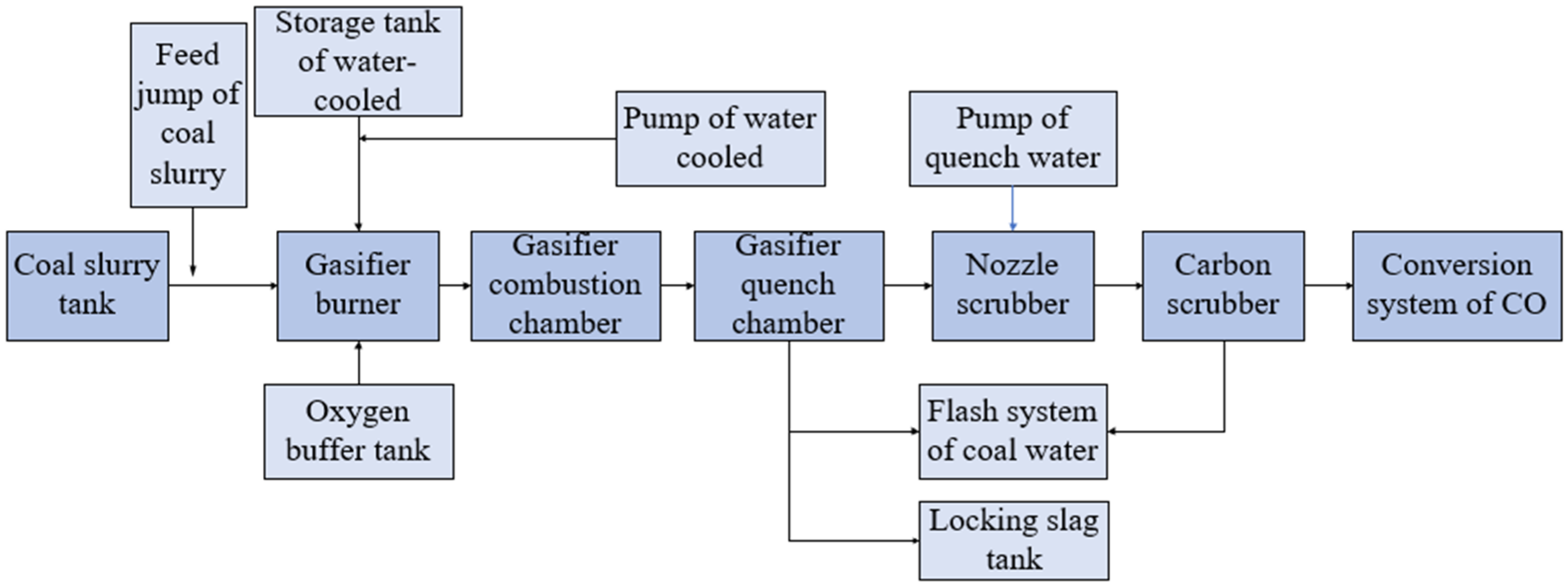
4. Application for Failure Assessment of a Coal Gasifier
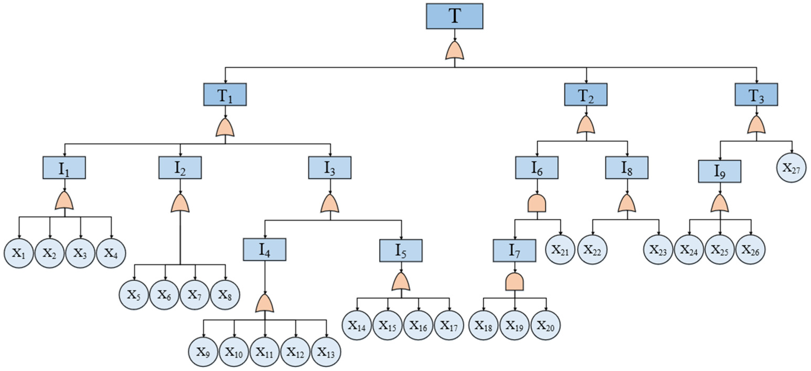
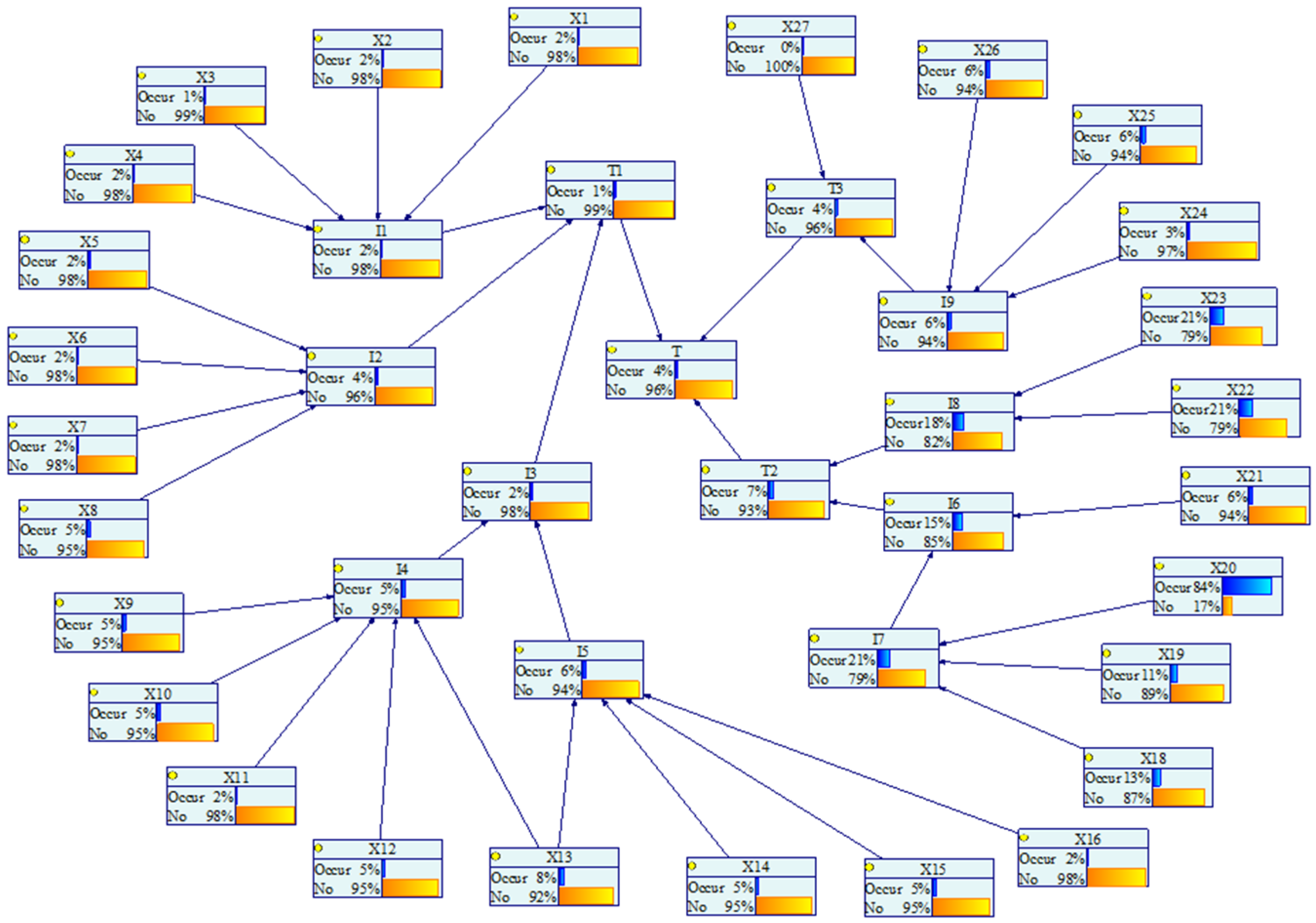
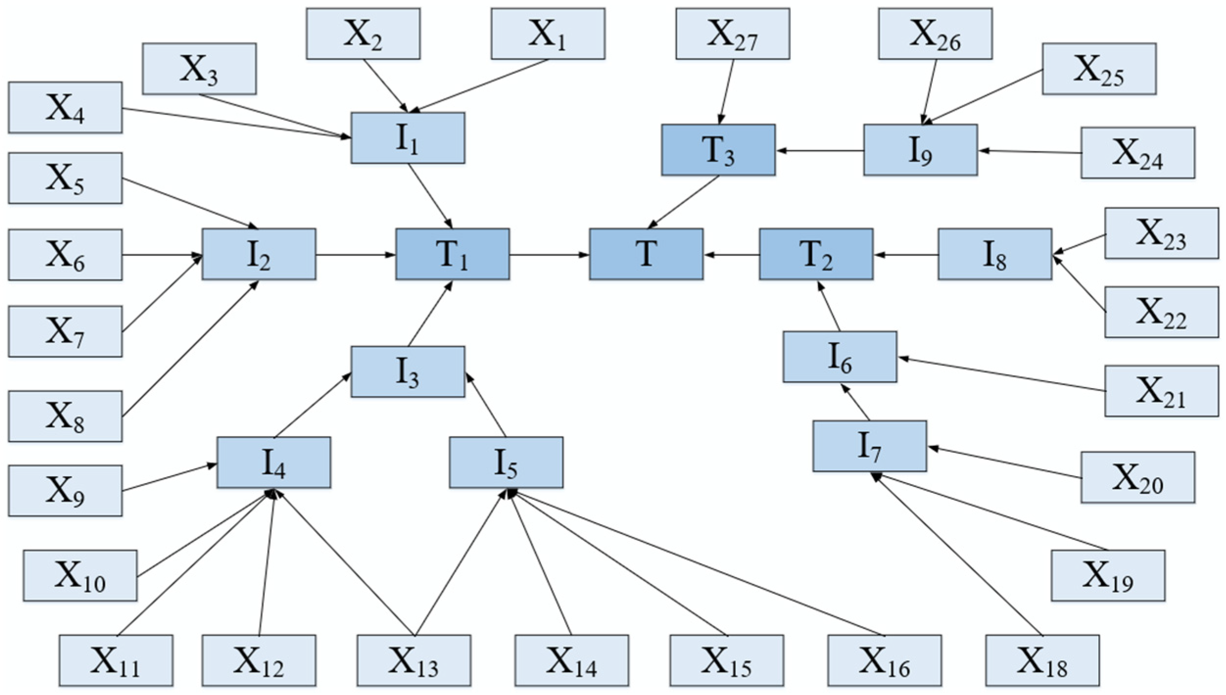
4.1. Construction of the BN for Analyzing the Failure Risk of the Gasifier
4.2. Collection of Experts’ Opinions on the Failure of the Coal Gasifier
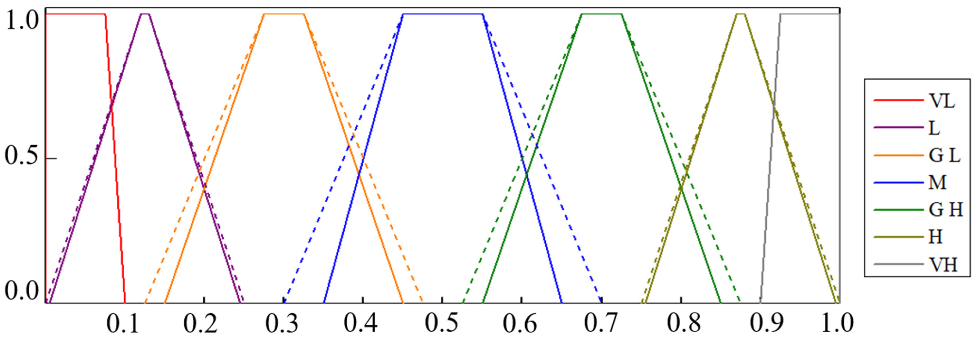
4.2.1. Definition of the TpIFN–Probabilistic Linguistic Scales
4.2.2. Expert’s Opinions on Root Events of the BN
4.3. Aggregation of the TpIFNs for Describing the Failure Probabilities of the Root Nodes
4.3.1. Calculation of the Experts’ Weights
4.3.2. Aggregation of the Experts’ Opinions
4.4. TpIFN-Defuzzification
4.4.1. Conversion of the TpIFNs into PSs
4.4.2. Determination of the FPs of All Root Nodes
4.5. BN Analysis
4.5.1. Prediction of the Failure Probability of the Gasifier
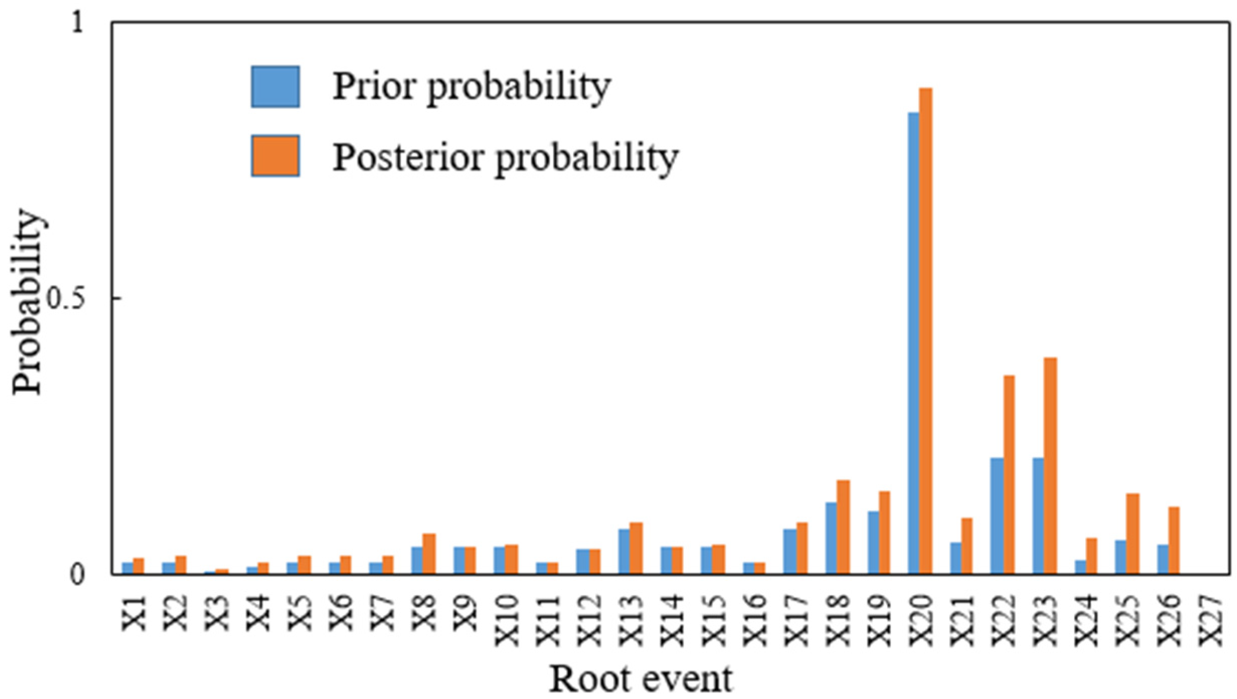
4.5.2. Diagnosis of the Key Nodes for the Failure of the Coal Gasifier
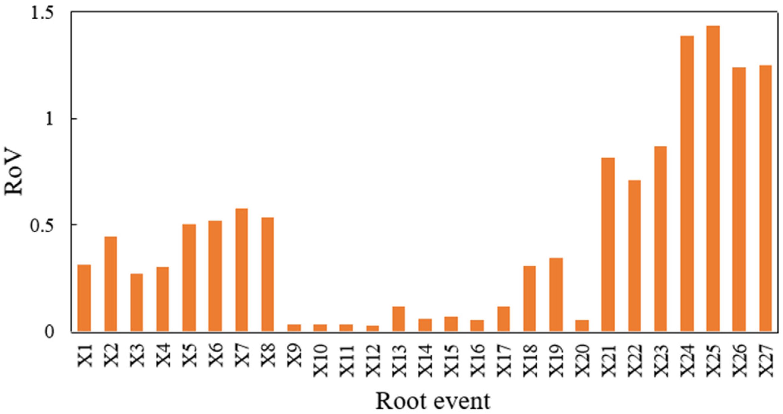
4.5.3. SA and CIA
5. Conclusions
- This framework combined the Bayesian network with the TpIFN-SAM to provide an alternative strategy for obtaining the prior probabilities of the root events in BNs.
- A set of TpIFNs was defined to quantify the linguistic terms for describing the failure possibilities of the events in BNs, which are more general and expressive than TpIFNs.
- The TpIFN-SAM can effectively aggregate the expert opinions on the prior probabilities of the root events in BNs and reduce the uncertain cumulative effect of the aggregation process by taking the effect of individual discrepancies into account for the consistency. The bidirectional reasoning of the BN coupled with sensitivity analysis can accurately calculate the system-failure probability and identify the key influencing factors that may lead to accidents.
Author Contributions
Funding
Data Availability Statement
Acknowledgments
Conflicts of Interest
Appendix A
- When k = 0, empty.
- When k > 0, let be a trapezoidal intuitionistic fuzzy number, and k is a real number, which we can know by Definition 2:The expected value of is
- When k < 0, same result as B. □
Appendix B

| X5 | X6 | X7 | X8 | I2 | |
|---|---|---|---|---|---|
| Occ | Non | ||||
| Occ | Occ | Occ | Occ | 1.00 | 0.00 |
| Occ | Occ | Occ | Non | 0.83 | 0.17 |
| Occ | Occ | Non | Occ | 0.86 | 0.14 |
| Occ | Non | Occ | Occ | 0.81 | 0.19 |
| Occ | Non | Occ | Non | 0.73 | 0.27 |
| Occ | Non | Non | Occ | 0.71 | 0.29 |
| Occ | Occ | Non | Non | 0.68 | 0.32 |
| Occ | Non | Non | Non | 0.35 | 0.65 |
| Non | Occ | Occ | Occ | 0.76 | 0.24 |
| Non | Occ | Occ | Non | 0.69 | 0.31 |
| Non | Occ | Non | Occ | 0.70 | 0.30 |
| Non | Occ | Non | Non | 0.36 | 0.64 |
| Non | Non | Occ | Occ | 0.69 | 0.31 |
| Non | Non | Occ | Non | 0.40 | 0.60 |
| Non | Non | Non | Occ | 0.38 | 0.62 |
| Non | Non | Non | Non | 0.00 | 1.00 |
| E4 | E5 | I3 | |
|---|---|---|---|
| Occ | Non | ||
| Occ | Occ | 1.00 | 0.00 |
| Occ | Non | 0.13 | 0.87 |
| Non | Occ | 0.17 | 0.83 |
| Non | Non | 0.00 | 1.00 |
| X9 | X10 | X11 | X12 | X13 | I4 | |
|---|---|---|---|---|---|---|
| Occ | Non | |||||
| Occ | Occ | Occ | Occ | Occ | 1.00 | 0.00 |
| Occ | Occ | Occ | Occ | Non | 0.75 | 0.25 |
| Occ | Occ | Occ | Non | Occ | 0.66 | 0.34 |
| Occ | Occ | Non | Occ | Occ | 0.60 | 0.40 |
| Occ | Non | Occ | Occ | Occ | 0.47 | 0.53 |
| Non | Occ | Occ | Occ | Occ | 0.45 | 0.55 |
| Occ | Occ | Occ | Non | Non | 0.53 | 0.47 |
| Occ | Occ | Non | Occ | Non | 0.49 | 0.51 |
| Occ | Non | Occ | Occ | Non | 0.43 | 0.57 |
| Non | Occ | Occ | Occ | Non | 0.39 | 0.61 |
| Occ | Occ | Non | Non | Occ | 0.51 | 0.49 |
| Occ | Non | Occ | Non | Occ | 0.43 | 0.57 |
| Non | Occ | Occ | Non | Occ | 0.40 | 0.60 |
| Occ | Non | Non | Occ | Occ | 0.38 | 0.62 |
| Non | Occ | Non | Occ | Occ | 0.34 | 0.66 |
| Non | Non | Occ | Occ | Occ | 0.30 | 0.70 |
| Oc | Occ | Non | Non | Non | 0.49 | 0.51 |
| Occ | Non | Occ | Non | Non | 0.42 | 0.58 |
| Non | Occ | Occ | Non | Non | 0.38 | 0.62 |
| Occ | Non | Non | Occ | Non | 0.37 | 0.63 |
| Non | Occ | Non | Occ | Non | 0.34 | 0.66 |
| Non | Non | Occ | Occ | Non | 0.29 | 0.71 |
| Occ | Non | Non | Non | Occ | 0.35 | 0.65 |
| Non | Occ | Non | Non | Occ | 0.33 | 0.67 |
| Non | Non | Occ | Non | Occ | 0.27 | 0.73 |
| Non | Non | Non | Occ | Occ | 0.25 | 0.75 |
| Occ | Non | Non | Non | Non | 0.19 | 0.81 |
| Non | Occ | Non | Non | Non | 0.21 | 0.79 |
| Non | Non | Occ | Non | Non | 0.24 | 0.76 |
| Non | Non | Non | Occ | Non | 0.20 | 0.80 |
| Non | Non | Non | Non | Occ | 0.25 | 0.75 |
| Non | Non | Non | Non | Non | 0.00 | 1.00 |
| X14 | X15 | X16 | X17 | I5 | |
|---|---|---|---|---|---|
| Occ | Non | ||||
| Occ | Occ | Occ | Occ | 1.00 | 0.00 |
| Occ | Occ | Occ | Non | 0.89 | 0.11 |
| Occ | Occ | Non | Occ | 0.83 | 0.17 |
| Occ | Non | Occ | Occ | 0.85 | 0.15 |
| Occ | Non | Occ | Non | 0.79 | 0.21 |
| Occ | Non | Non | Occ | 0.76 | 0.24 |
| Occ | Occ | Non | Non | 0.68 | 0.32 |
| Occ | Non | Non | Non | 0.32 | 0.68 |
| Non | Occ | Occ | Occ | 0.86 | 0.14 |
| Non | Occ | Occ | Non | 0.71 | 0.29 |
| Non | Occ | Non | Occ | 0.69 | 0.31 |
| Non | Occ | Non | Non | 0.37 | 0.63 |
| Non | Non | Occ | Occ | 0.42 | 0.58 |
| Non | Non | Occ | Non | 0.28 | 0.72 |
| Non | Non | Non | Occ | 0.26 | 0.74 |
| Non | Non | Non | Non | 0.00 | 1.00 |
| E7 | X21 | I6 | |
|---|---|---|---|
| Occ | Non | ||
| Occ | Occ | 1.00 | 0.00 |
| Occ | Non | 0.65 | 0.35 |
| Non | Occ | 0.33 | 0.67 |
| Non | Non | 0.00 | 1.00 |
| X18 | X19 | X20 | I7 | |
|---|---|---|---|---|
| Occ | Non | |||
| Occ | Occ | Occ | 1.00 | 0.00 |
| Occ | Occ | Non | 0.35 | 0.65 |
| Occ | Non | Occ | 0.36 | 0.64 |
| Occ | Non | Non | 0.15 | 0.85 |
| Non | Occ | Occ | 0.37 | 0.63 |
| Non | Occ | Non | 0.17 | 0.83 |
| Non | Non | Occ | 0.19 | 0.81 |
| Non | Non | Non | 0.00 | 1.00 |
| X22 | X23 | I8 | |
|---|---|---|---|
| Occ | Non | ||
| Occ | Occ | 1.00 | 0.00 |
| Occ | Non | 0.45 | 0.55 |
| Non | Occ | 0.36 | 0.64 |
| Non | Non | 0.00 | 1.00 |
| X24 | X25 | X26 | I9 | |
|---|---|---|---|---|
| Occ | Non | |||
| Occ | Occ | Occ | 1.00 | 0.00 |
| Occ | Occ | Non | 0.67 | 0.33 |
| Occ | Non | Occ | 0.71 | 0.29 |
| Occ | Non | Non | 0.35 | 0.65 |
| Non | Oc | Occ | 0.69 | 0.31 |
| Non | Occ | Non | 0.41 | 0.59 |
| Non | Non | Occ | 0.38 | 0.62 |
| Non | Non | Non | 0.00 | 1.00 |
| E1 | E2 | E3 | T1 | |
|---|---|---|---|---|
| Occ | Non | |||
| Occ | Occ | Occ | 1.00 | 0.00 |
| Occ | Occ | Non | 0.22 | 0.78 |
| Occ | Non | Occ | 0.33 | 0.67 |
| Occ | Non | Non | 0.18 | 0.82 |
| Non | Occ | Occ | 0.32 | 0.68 |
| Non | Occ | Non | 0.19 | 0.81 |
| Non | Non | Occ | 0.13 | 0.87 |
| Non | Non | Non | 0.00 | 1.00 |
| E6 | E8 | T2 | |
|---|---|---|---|
| Occ | Non | ||
| Occ | Occ | 1.00 | 0.00 |
| Occ | Non | 0.17 | 0.83 |
| Non | Occ | 0.15 | 0.85 |
| Non | Non | 0.00 | 1.00 |
| E9 | X27 | T3 | |
|---|---|---|---|
| Occ | Non | ||
| Occ | Occ | 1.00 | 0.00 |
| Occ | Non | 0.66 | 0.34 |
| Non | Occ | 0.21 | 0.79 |
| Non | Non | 0.00 | 1.00 |
| T1 | T2 | T3 | T | |
|---|---|---|---|---|
| Occ | N | |||
| Occ | Occ | Occ | 1.00 | 0.00 |
| Occ | Occ | Non | 0.28 | 0.72 |
| Occ | Non | Occ | 0.37 | 0.63 |
| Occ | Non | Non | 0.33 | 0.67 |
| Non | Occ | Occ | 0.38 | 0.62 |
| Non | Occ | Non | 0.34 | 0.66 |
| Non | Non | Occ | 0.23 | 0.77 |
| Non | Non | Non | 0.00 | 1.00 |
References
- Cao, C.; Zhang, Y.; Yu, T.; Gu, X.; Xin, Z.; Li, J. A Novel 3-Layer Mixed Cultural Evolutionary Optimization Framework for Optimal Operation of Syngas Production in a Texaco Coal-Water Slurry Gasifier. Chin. J. Chem. Eng. 2015, 23, 1484–1501. [Google Scholar] [CrossRef]
- Ashraf, A.M.; Imran, W.; Véchot, L. Analysis of the Impact of a Pandemic on the Control of the Process Safety Risk in Major Hazards Industries Using a Fault Tree Analysis Approach. J. Loss Prev. Process Ind. 2022, 74, 104649. [Google Scholar] [CrossRef] [PubMed]
- Hong, E.-S.; Lee, I.-M.; Shin, H.-S.; Nam, S.-W.; Kong, J.-S. Quantitative Risk Evaluation Based on Event Tree Analysis Technique: Application to the Design of Shield TBM. Tunn. Undergr. Space Technol. 2009, 24, 269–277. [Google Scholar] [CrossRef]
- Wang, W.; Mou, D.; Li, F.; Dong, C.; Khan, F. Dynamic Failure Probability Analysis of Urban Gas Pipeline Network. J. Loss Prev. Process Ind. 2021, 72, 104552. [Google Scholar] [CrossRef]
- George, P.G.; Renjith, V.R. Evolution of Safety and Security Risk Assessment Methodologies towards the Use of Bayesian Networks in Process Industries. Process Saf. Environ. Prot. 2021, 149, 758–775. [Google Scholar] [CrossRef]
- Khakzad, N.; Khan, F.; Amyotte, P. Safety Analysis in Process Facilities: Comparison of Fault Tree and Bayesian Network Approaches. Reliab. Eng. Syst. Saf. 2011, 96, 925–932. [Google Scholar] [CrossRef]
- Bhandari, J.; Abbassi, R.; Garaniya, V.; Khan, F. Risk Analysis of Deepwater Drilling Operations Using Bayesian Network. J. Loss Prev. Process Ind. 2015, 38, 11–23. [Google Scholar] [CrossRef]
- Yazdi, M.; Khan, F.; Abbassi, R.; Quddus, N. Resilience Assessment of a Subsea Pipeline Using Dynamic Bayesian Network. J. Pipeline Sci. Eng. 2022, 2, 100053. [Google Scholar] [CrossRef]
- Eleye-Datubo, A.G.; Wall, A.; Wang, J. Marine and Offshore Safety Assessment by Incorporative Risk Modeling in a Fuzzy-Bayesian Network of an Induced Mass Assignment Paradigm. Risk Anal. 2008, 28, 95–112. [Google Scholar] [CrossRef]
- Xu, B.; Hu, J.; Hu, T.; Wang, F.; Luo, K.; Wang, Q.; He, X. Quantitative Assessment of Seismic Risk in Hydraulic Fracturing Areas Based on Rough Set and Bayesian Network: A Case Analysis of Changning Shale Gas Development Block in Yibin City, Sichuan Province, China. J. Pet. Sci. Eng. 2021, 200, 108226. [Google Scholar] [CrossRef]
- Yazdi, M.; Kabir, S. Fuzzy Evidence Theory and Bayesian Networks for Process Systems Risk Analysis. Hum. Ecol. Risk Assess. Int. J. 2020, 26, 57–86. [Google Scholar] [CrossRef]
- Gao, P.; Li, W.; Sun, Y.; Liu, S. Risk Assessment for Gas Transmission Station Based on Cloud Model Based Multilevel Bayesian Network from the Perspective of Multi-Flow Intersecting Theory. Process Saf. Environ. Prot. 2022, 159, 887–898. [Google Scholar] [CrossRef]
- Zhu, M.; Chen, D.; Wang, J.; Wang, J.; Sun, Y. Analysis of Oceanaut Operating Performance Using an Integrated Bayesian Network Aided by the Fuzzy Logic Theory. Int. J. Ind. Ergon. 2021, 83, 103129. [Google Scholar] [CrossRef]
- Zarei, E.; Khakzad, N.; Cozzani, V.; Reniers, G. Safety Analysis of Process Systems Using Fuzzy Bayesian Network (FBN). J. Loss Prev. Process Ind. 2019, 57, 7–16. [Google Scholar] [CrossRef]
- Kabir, G.; Sadiq, R.; Tesfamariam, S. A Fuzzy Bayesian Belief Network for Safety Assessment of Oil and Gas Pipelines. Struct. Infrastruct. Eng. 2016, 12, 874–889. [Google Scholar] [CrossRef]
- Yazdi, M.; Kabir, S. A Fuzzy Bayesian Network Approach for Risk Analysis in Process Industries. Process Saf. Environ. Prot. 2017, 111, 507–519. [Google Scholar] [CrossRef]
- Zhao, D.; Wang, Z.; Song, Z.; Guo, P.; Cao, X. Assessment of Domino Effects in the Coal Gasification Process Using Fuzzy Analytic Hierarchy Process and Bayesian Network. Saf. Sci. 2020, 130, 104888. [Google Scholar] [CrossRef]
- Yan, F.; Xu, K.; Yao, X.; Li, Y. Fuzzy Bayesian Network-Bow-Tie Analysis of Gas Leakage during Biomass Gasification. PLoS ONE 2016, 11, e0160045. [Google Scholar] [CrossRef]
- Pouyakian, M.; Jafari, M.J.; Laal, F.; Nourai, F.; Zarei, E. A Comprehensive Approach to Analyze the Risk of Floating Roof Storage Tanks. Process Saf. Environ. Prot. 2021, 146, 811–836. [Google Scholar] [CrossRef]
- Rostamabadi, A.; Jahangiri, M.; Zarei, E.; Kamalinia, M.; Alimohammadlou, M. A Novel Fuzzy Bayesian Network Approach for Safety Analysis of Process Systems; An Application of HFACS and SHIPP Methodology. J. Clean. Prod. 2020, 244, 118761. [Google Scholar] [CrossRef]
- Uluçay, V.; Deli, I.; Şahin, M. Trapezoidal Fuzzy Multi-Number and Its Application to Multi-Criteria Decision-Making Problems. Neural Comput. Appl. 2018, 30, 1469–1478. [Google Scholar] [CrossRef]
- Uluay, V. A New Similarity Function of Trapezoidal Fuzzy Multi-Numbers Based on Multi-Criteria Decision Making. J. Inst. Sci. Tech. 2020, 2020, 1233–1246. [Google Scholar] [CrossRef]
- Atanassov, K.T. Intuitionistic fuzzy sets. J. Fuzzy Sets Syst. 1986, 20, 87–96. [Google Scholar] [CrossRef]
- Yu, J.; Wu, S.; Yu, Y.; Chen, H.; Fan, H.; Liu, J.; Ge, S. Process System Failure Evaluation Method Based on a Noisy-OR Gate Intuitionistic Fuzzy Bayesian Network in an Uncertain Environment. Process Saf. Environ. Prot. 2021, 150, 281–297. [Google Scholar] [CrossRef]
- Kumar, M.; Kaushik, M. System Failure Probability Evaluation Using Fault Tree Analysis and Expert Opinions in Intuitionistic Fuzzy Environment. J. Loss Prev. Process Ind. 2020, 67, 104236. [Google Scholar] [CrossRef]
- Hsu, H.-M.; Chen, C.-T. Aggregation of Fuzzy Opinions under Group Decision Making. Fuzzy Sets Syst. 1996, 79, 279–285. [Google Scholar] [CrossRef]
- Kim, H.; Koh, J.-S.; Kim, Y.; Theofanous, T.G. Risk Assessment of Membrane Type LNG Storage Tanks in Korea-Based on Fault Tree Analysis. Korean J. Chem. Eng. 2005, 22, 1–8. [Google Scholar] [CrossRef]
- Yazdi, M. Hybrid Probabilistic Risk Assessment Using Fuzzy FTA and Fuzzy AHP in a Process Industry. J. Fail. Anal. Prev. 2017, 17, 756–764. [Google Scholar] [CrossRef]
- Yin, H.; Liu, C.; Wu, W.; Song, K.; Liu, D.; Dan, Y. Safety Assessment of Natural Gas Storage Tank Using Similarity Aggregation Method Based Fuzzy Fault Tree Analysis (SAM-FFTA) Approach. J. Loss Prev. Process Ind. 2020, 66, 104159. [Google Scholar] [CrossRef]
- Yin, H.; Liu, C.; Wu, W.; Song, K.; Dan, Y.; Cheng, G. An Integrated Framework for Criticality Evaluation of Oil & Gas Pipelines Based on Fuzzy Logic Inference and Machine Learning. J. Nat. Gas Sci. Eng. 2021, 96, 104264. [Google Scholar] [CrossRef]
- Kabir, S.; Papadopoulos, Y. A Review of Applications of Fuzzy Sets to Safety and Reliability Engineering. Int. J. Approx. Reason. 2018, 100, 29–55. [Google Scholar] [CrossRef]
- Uluçay, V.; Deli, I.; Şahin, M. Intuitionistic Trapezoidal Fuzzy Multi-Numbers and Its Application to Multi-Criteria Decision-Making Problems. Complex Intell. Syst. 2019, 5, 65–78. [Google Scholar] [CrossRef]
- Li, X.; Chen, X. Multi-Criteria Group Decision Making Based on Trapezoidal Intuitionistic Fuzzy Information. Appl. Soft Comput. 2015, 30, 454–461. [Google Scholar] [CrossRef]
- Wang, J.; Zhong, Z. Aggregation operators on intuitionistic trapezoidal fuzzy number and its application to multi-criteria decision making problems. J. Syst. Eng. Elect. 2009, 20, 321–326. [Google Scholar] [CrossRef]
- Heilpern, S. The expected value of a fuzzy number. J. Fuzzy Sets Syst. 1992, 47, 81–86. [Google Scholar] [CrossRef]
- Bharati, S.K.; Malhotra, R. Two Stage Intuitionistic Fuzzy Time Minimizing Transportation Problem Based on Generalized Zadeh’s Extension Principle. Int. J. Syst. Assur. Eng. Manag. 2017, 8, 1442–1449. [Google Scholar] [CrossRef]
- Kabir, S.; Papadopoulos, Y. Applications of Bayesian Networks and Petri Nets in Safety, Reliability, and Risk Assessments: A Review. Saf. Sci. 2019, 115, 154–175. [Google Scholar] [CrossRef]
- Bulmer, R.H.; Stephenson, F.; Lohrer, A.M.; Lundquist, C.J.; Madarasz-Smith, A.; Pilditch, C.A.; Thrush, S.F.; Hewitt, J.E. Informing the Management of Multiple Stressors on Estuarine Ecosystems Using an Expert-Based Bayesian Network Model. J. Environ. Manag. 2022, 301, 113576. [Google Scholar] [CrossRef]
- Zhou, Y.; Li, C.; Zhou, C.; Luo, H. Using Bayesian Network for Safety Risk Analysis of Diaphragm Wall Deflection Based on Field Data. Reliab. Eng. Syst. Saf. 2018, 180, 152–167. [Google Scholar] [CrossRef]
- Bobbio, A.; Portinale, L.; Minichino, M.; Ciancamerla, E. Improving the Analysis of Dependable Systems by Mapping Fault Trees into Bayesian Networks. Reliab. Eng. Syst. Saf. 2001, 71, 249–260. [Google Scholar] [CrossRef]
- Zhang, C.; Wu, J.; Hu, X.; Ni, S. A Probabilistic Analysis Model of Oil Pipeline Accidents Based on an Integrated Event-Evolution-Bayesian (EEB) Model. Process Saf. Environ. Prot. 2018, 117, 694–703. [Google Scholar] [CrossRef]
- Dimaio, F.; Scapinello, O.; Zio, E.; Ciarapica, C.; Cincotta, S.; Crivellari, A.; Decarli, L.; Larosa, L. Accounting for Safety Barriers Degradation in the Risk Assessment of Oil and Gas Systems by Multistate Bayesian Networks. Reliab. Eng. Syst. Saf. 2021, 216, 107943. [Google Scholar] [CrossRef]
- Nicolis, J.S.; Tsuda, I. Chaotic dynamics of information processing: The “magic number seven plus-minus two” revisited. J. Bull. Math. Biol. 1985, 47, 343–365. [Google Scholar] [CrossRef]
- Ishikawa, A.; Amagasa, M.; Shiga, T.; Tomizawa, G.; Tatsuta, R.; Mieno, H. The Max-Min Delphi Method and Fuzzy Delphi Method via Fuzzy Integration. Fuzzy Sets Syst. 1993, 55, 241–253. [Google Scholar] [CrossRef]
- Saaty, T.L.; Vargas, L.G. Estimating Technological Coefficients by the Analytic Hierarchy Process. Socioecon. Plann. Sci. 1979, 13, 333–336. [Google Scholar] [CrossRef]
- Xu, Z.; Liao, H. Intuitionistic Fuzzy Analytic Hierarchy Process. IEEE Trans. Fuzzy Syst. 2014, 22, 749–761. [Google Scholar] [CrossRef]
- Onisawa, T. A Representation of Human Reliability Using Fuzzy Concepts. Inf. Sci. 1988, 45, 153–173. [Google Scholar] [CrossRef]
- Yu, J.; Chen, H.; Yu, Y.; Yang, Z. A Weakest T-Norm Based Fuzzy Fault Tree Approach for Leakage Risk Assessment of Submarine Pipeline. J. Loss Prev. Process Ind. 2019, 62, 103–968. [Google Scholar] [CrossRef]
- Kwan, M.; Overill, R.; Chow, K.-P.; Tse, H.; Law, F.; Lai, P. Sensitivity Analysis of Bayesian Networks Used in Forensic Investigations. In Advances in Digital Forensics VII; IFIP Advances in Information and Communication Technology; Peterson, G., Shenoi, S., Eds.; Springer: Berlin/Heidelberg, Germany, 2011; Volume 361, pp. 231–243. ISBN 978-3-642-24211-3. [Google Scholar]


| X1 | Occ | Non | |||||||
|---|---|---|---|---|---|---|---|---|---|
| X2 | Occ | Non | Occ | Non | |||||
| X3 | Occ | Non | Occ | Non | Occ | Non | Occ | Non | |
| T | Occ | 1 | 0 | 0 | 0 | 0 | 0 | 0 | 0 |
| Non | 0 | 1 | 1 | 1 | 1 | 1 | 1 | 1 | |
| X1 | Occ | Non | |||||||
|---|---|---|---|---|---|---|---|---|---|
| X2 | Occ | Non | Occ | Non | |||||
| X3 | Occ | Non | Occ | Non | Occ | Non | Occ | Non | |
| T | Occ | 1 | 1 | 1 | 1 | 1 | 1 | 1 | 0 |
| Non | 0 | 1 | 1 | 1 | 1 | 1 | 1 | 1 | |
| Level | IFNs |
|---|---|
| i is significantly important than j. | μ = 0.9, ν = 0–0.1 |
| i is much more important than j. | μ = 0.8, ν = 0–0.2 |
| I is more important than j. | μ = 0.7, ν = 0–0.3 |
| i is slightly more important than j. | μ = 0.6, ν = 0–0.4 |
| i is as important as j. | μ = ν |
| T/IEs | Description | REs | Description | REs | Description |
|---|---|---|---|---|---|
| T | Gasifier failure | X1 | Slag opening blocked by large pieces of slag | X14 | Low oxygen-flow rate |
| T1 | Gasifier abnormality | X2 | Slag opening blocked by molten furnace bricks | X15 | High flow rate of coal slurry |
| T2 | Corrosion failure | X3 | Low liquid level in quench chamber | X16 | High concentration of coal slurry |
| T3 | Human organization factors | X4 | Cracking in the quench ring or vertical pipe | X17 | Temperature sensor damaged |
| I1 | Pressure fluctuation | X5 | Abnormal flow rate of quench water | X18 | High H2S content |
| I2 | Abnormal liquid level | X6 | Abnormal flow rate of coal water | X19 | High CO2 content |
| I3 | Abnormal temperature | X7 | Leakage of drain valve of quench water | X20 | High H2O content |
| I4 | Too-high temperature | X8 | Liquid-level gauge damaged by blockage | X21 | High flow rate |
| I5 | Too-low temperature | X9 | High oxygen-flow rate | X22 | Anti-corrosion layer damaged |
| I6 | Internal corrosion | X10 | Low flow rate of coal slurry | X23 | Insulation layer damaged |
| I7 | Medium content | X11 | Low concentration of coal slurry | X24 | Pre-job training is not up to standard |
| I8 | External corrosion | X12 | Burner damaged | X25 | Improper operation |
| I9 | Unintentional destruction | X13 | Temperature sensor damaged | X26 | Unattended (unsafe supervision) |
| X27 | Deliberate destruction |
| Level | Description | Failure Probability |
|---|---|---|
| Quite Low | No expected failures over the entire operating life of the equipment. | <10−5 |
| Low | ≥1 accident may occur during the entire operating life of the equipment. | 10−5–10−4 |
| Ordinary Low | ≥1 accident may occur within 10 years of equipment operation. | 10−4–5 × 10⁻⁴ |
| Moderate | ≥1 accident may occur within 5 years of equipment operation. | 5 × 10⁻⁴–2 × 10⁻³ |
| Odinary High | ≥1 accident may occur per year of equipment operation. | 2 × 10⁻³–10−2 |
| High | ≥1 accident may occur per quarter of equipment operation. | 10−2–10−1 |
| Quite High | ≥1 accident may occur per month of equipment operation. | >10−1 |
| Failure Possibility | Trapezoidal Intuitionistic Fuzzy Number |
|---|---|
| Quite Low | (0, 0, 0.075, 0.1; 0, 0, 0.075, 0.1) |
| Low | (0.005, 0.12, 0.13, 0.245; 0, 0.12, 0.13, 0.25) |
| Ordinary Low | (0.15, 0.275, 0.325, 0.45; 0.125, 0.275, 0.325, 0.475) |
| Moderate | (0.35, 0.45, 0.55, 0.65; 0.3, 0.45, 0.55, 0.7) |
| Ordinary High | (0.55, 0.675, 0.725, 0.85; 0.525, 0.675, 0.725, 0.875) |
| High | (0.755, 0.87, 0.88, 0.995; 0.75, 0.87, 0.88, 1) |
| Quite High | (0.9, 0.925, 1, 1; 0.9, 0.925, 1, 1) |
| Event | Linguistic Judgment of Experts | Event | Linguistic Judgment of Experts | ||||||
|---|---|---|---|---|---|---|---|---|---|
| E1 | E2 | E3 | E4 | E1 | E2 | E3 | E4 | ||
| X1 | OL | MO | OL | MO | X15 | OL | MO | MO | MO |
| X2 | MO | OL | OL | MO | X16 | MO | MO | OL | OL |
| X3 | OL | LO | OL | OL | X17 | MO | OH | MO | MO |
| X4 | OL | OL | OL | MO | X18 | MO | OH | MO | OH |
| X5 | MO | MO | OL | OL | X19 | OH | MO | OH | MO |
| X6 | MO | MO | OL | OL | X20 | HI | HI | HI | HI |
| X7 | MO | MO | OL | OL | X21 | MO | MO | OL | MO |
| X8 | MO | MO | MO | MO | X22 | OH | OH | MO | OH |
| X9 | MO | OL | MO | MO | X23 | OH | MO | OH | OH |
| X10 | OL | MO | MO | MO | X24 | OL | OL | MO | MO |
| X11 | MO | MO | OL | OL | X25 | MO | MO | OL | MO |
| X12 | OL | MO | MO | OL | X26 | OL | MO | MO | MO |
| X13 | MO | MO | MO | OH | X27 | LO | LO | QL | LO |
| X14 | OL | MO | MO | MO | |||||
| Professional Position | Education Level | Service Time | |
|---|---|---|---|
| E1 | Professor | Doctorate | 30 |
| E2 | Engineer | Master’s | 24 |
| E3 | Associate professor | Doctorate | 23 |
| E4 | Engineer | Bachelor’s | 32 |
| R | C1 | C2 | C3 |
|---|---|---|---|
| C1 | (0.5, 0.5) | (0.7, 0.2) | (0.6, 0.2) |
| C2 | (0.2, 0.7) | (0.5, 0.5) | (0.2, 0.6) |
| C3 | (0.2, 0.6) | (0.6, 0.2) | (0.5, 0.5) |
| R1 | E1 | E2 | E3 | E4 |
|---|---|---|---|---|
| E1 | (0.5, 0.5) | (0.7, 0.2) | (0.6, 0.3) | (0.7, 0.2) |
| E2 | (0.3, 0.6) | (0.5, 0.5) | (0.3, 0.6) | (0.4, 0.4) |
| E3 | (0.3, 0.6) | (0.6, 0.3) | (0.5, 0.5) | (0.6, 0.3) |
| E4 | (0.2, 0.7) | (0.4, 0.4) | (0.3, 0.6) | (0.5, 0.5) |
| R2 | E1 | E2 | E3 | E4 |
|---|---|---|---|---|
| E1 | (0.5, 0.5) | (0.7, 0.2) | (0.4, 0.4) | (0.7, 0.1) |
| E2 | (0.2, 0.7) | (0.5, 0.5) | (0.7, 0.2) | (0.6, 0.2) |
| E3 | (0.4, 0.4) | (0.2, 0.7) | (0.5, 0.5) | (0.7, 0.1) |
| E4 | (0.1, 0.7) | (0.2, 0.6) | (0.1, 0.7) | (0.5, 0.5) |
| R3 | E1 | E2 | E3 | E4 |
|---|---|---|---|---|
| E1 | (0.5, 0.5) | (0.6, 0.2) | (0.6, 0.2) | (0.4, 0.4) |
| E2 | (0.2, 0.6) | (0.5, 0.5) | (0.3, 0.3) | (0.2, 0.6) |
| E3 | (0.2, 0.6) | (0.3, 0.3) | (0.5, 0.5) | (0.2, 0.6) |
| E4 | (0.4, 0.4) | (0.6, 0.2) | (0.6, 0.2) | (0.5, 0.5) |
| εi | C1 | C2 | C3 | Wj |
|---|---|---|---|---|
| (0.315, 0.602) | (0.176, 0.602) | (0.265, 0.632) | ||
| E1 | (0.284, 0.622) | (0.256, 0.6) | (0.223, 0.591) | (0.182, 0.607) |
| E2 | (0.171, 0.742) | (0.222, 0.657) | (0.128, 0.697) | (0.122, 0.688) |
| E3 | (0.227, 0.689) | (0.2, 0.671) | (0.128, 0.697) | (0.135, 0.677) |
| E4 | (0.159, 0.757) | (0.1, 0.786) | (0.223, 0.591) | (0.122, 0.702) |
| Subject | Data | Subject | Data | Process |
|---|---|---|---|---|
| (0.38, 0.46, 0.57, 0.63; 0.32, 0.46, 0.56, 0.68) | 0.509 | |||
| (0.56, 0.68, 0.74, 0.83; 0.53, 0.68, 0.74, 0.85) | 0.701 | |||
| (0.39, 0.47, 0.58, 0.64; 0.33, 0.47, 0.58, 0.69) | 0.519 | |||
| (0.57, 0.69, 0.75, 0.84; 0.54, 0.69, 0.75, 0.86) | 0.711 | |||
| 0.726 | 0.740 | |||
| 0.981 | 0.986 | |||
| 0.715 | 0.729 | |||
| WA (E1) | 0.821 | |||
| WA (E2) | 0.825 | |||
| WA (E3) | 0.832 | |||
| WA (E4) | 0.817 | |||
| RAD (E1) | 0.249 | |||
| RAD (E2) | 0.334 | |||
| RAD (E3) | 0.253 | |||
| RAD (E4) | 0.248 | |||
| CDC1 | 0.252 | |||
| CDC2 | 0.298 | |||
| CDC3 | 0.252 | |||
| CDC4 | 0.248 | |||
| Aggregation TpIFN | (0.502, 0.608, 0.697, 0.776; 0.456, 0.608, 0.697, 0.812) | CDCi = β·ω + (1 − β)·RADi | ||
| PS | 0.534 | |||
| FP | 1.30 × 10−³ | CDC1 = 0.4 × 0.257 + 0.6 × 0.249 = 0.252 | ||
| Events | Aggregated TpIFNs | PS | FP |
|---|---|---|---|
| X1 | (0.278, 0.361, 0.451, 0.547; 0.235, 0.361, 0.451, 0.599) | 0.312 | 2.36 × 10⁻⁴ |
| X2 | (0.278, 0, 0.361, 0.451, 0.547; 0.235, 0.361, 0.451, 0.599) | 0.312 | 2.36 × 10⁻⁴ |
| X3 | (0.111, 0.231, 0.273, 0.389; 0.082; 0.231, 0.273; 0.421) | 0.169 | 7.60 × 10⁻⁵ |
| X4 | (0.221, 0.323, 0.394, 0.506; 0.184, 0.323, 0.394, 0.556) | 0.267 | 1.67 × 10⁻⁴ |
| X5 | (0.281, 0.368, 0.437, 0.546; 0.234, 0.368, 0.437, 0.585) | 0.312 | 2.36 × 10⁻⁴ |
| X6 | (0.257, 0.349, 0.427, 0.530; 0.226, 0.349, 0.427, 0.569) | 0.301 | 2.17 × 10⁻⁴ |
| X7 | (0.251, 0.343, 0.421, 0.510; 0.240, 0.343, 0.421, 0.559) | 0.301 | 2.16 × 10⁻⁴ |
| X8 | (0.394, 0.447, 0.551, 0.668; 0.352, 0.447, 0.551, 0.726) | 0.407 | 4.91 × 10⁻⁴ |
| X9 | (0.415, 0.454, 0.561, 0.676; 0.343, 0.454, 0.561, 0.721) | 0.409 | 4.96 × 10⁻⁴ |
| X10 | (0.422, 0.459, 0.567, 0.679; 0.349, 0.459, 0.567, 0.712) | 0.416 | 5.26 × 10⁻⁴ |
| X11 | (0.248, 0.340, 0.417, 0.505; 0.236, 0.340, 0.417, 0.552) | 0.298 | 2.12 × 10⁻⁴ |
| X12 | (0.401, 0.438, 0.543, 0.661; 0.330, 0.438, 0.543, 0.689) | 0.399 | 4.61 × 10⁻⁴ |
| X13 | (0.487, 0.542, 0.657, 0.728; 0.399, 0.542, 0.657, 0.760) | 0.477 | 8.39 × 10⁻⁴ |
| X14 | (0.415, 0.454, 0.561, 0.676; 0.343, 0.454, 0.561, 0.721) | 0.409 | 4.96 × 10⁻⁴ |
| X15 | (0.422, 0.459, 0.567, 0.679; 0.349, 0.459, 0.567, 0.712) | 0.416 | 5.26 × 10⁻⁴ |
| X16 | (0.248, 0.340, 0.417, 0.505; 0.236, 0.340, 0.417, 0552) | 0.298 | 2.12 × 10⁻⁴ |
| X17 | (0.487, 0.542, 0.657, 0.728; 0.399, 0.542, 0.657, 0.760) | 0.477 | 8.39 × 10⁻⁴ |
| X18 | (0.502, 0.608, 0.697, 0.776; 0.456, 0.608, 0.697, 0.812) | 0.534 | 1.30 × 10⁻³ |
| X19 | (0.484, 0.587, 0.675, 0.755; 0.440, 0.587, 0.675, 0.791) | 0.517 | 1.14 × 10⁻³ |
| X20 | (0.814, 0.867, 0.909, 0.977; 0.768, 0.867, 0.909, 0.992) | 0.777 | 8.35 × 10⁻³ |
| X21 | (0.393, 0.504, 0.603, 0.666; 0.332, 0.504, 0.603, 0.716) | 0.428 | 5.74 × 10⁻⁴ |
| X22 | (0.561, 0.663, 0.743, 0.828; 0.532, 0.663, 0.743, 0.861) | 0.596 | 2.10 × 10⁻³ |
| X23 | (0.561, 0.663, 0.743, 0.828; 0.532, 0.663, 0.743, 0.861) | 0.596 | 2.10 × 10⁻³ |
| X24 | (0.297, 0.401, 0.488, 0.553; 0.245, 0.401, 0.488, 0.593) | 0.337 | 2.86 × 10⁻⁴ |
| X25 | (0.401, 0.467, 0.597, 0.669; 0.368, 0.467, 0.597, 0.705) | 0.436 | 6.12 × 10⁻⁴ |
| X26 | (0.396, 0.461, 0.579, 0.659; 0.357, 0.461, 0.579, 0.697) | 0.424 | 5.59 × 10⁻⁴ |
| X27 | (0.007, 0.113, 0.123, 0.224; 0.002, 0.113, 0.123, 0.241) | 0.061 | 1.40 × 10⁻⁵ |
| X1 | X2 | X3 | X4 | I1 | |
|---|---|---|---|---|---|
| Occ | Non | ||||
| Occ | Occ | Occ | Occ | 1.00 | 0.00 |
| Occ | Occ | Occ | Non | 0.67 | 0.33 |
| Occ | Occ | Non | Occ | 0.69 | 0.31 |
| Occ | Non | Occ | Occ | 0.72 | 0.28 |
| Occ | Non | Occ | Non | 0.62 | 0.38 |
| Occ | Non | Non | Occ | 0.58 | 0.42 |
| Occ | Occ | Non | Non | 0.57 | 0.43 |
| Occ | Non | Non | Non | 0.21 | 0.79 |
| Non | Occ | Occ | Occ | 0.85 | 0.15 |
| Non | Occ | Occ | Non | 0.67 | 0.33 |
| Non | Occ | Non | Occ | 0.68 | 0.32 |
| Non | Occ | Non | Non | 0.31 | 0.69 |
| Non | Non | Occ | Occ | 0.42 | 0.58 |
| Non | Non | Occ | Non | 0.18 | 0.82 |
| Non | Non | Non | Occ | 0.21 | 0.79 |
| Non | Non | Non | Non | 0.00 | 1.00 |
Publisher’s Note: MDPI stays neutral with regard to jurisdictional claims in published maps and institutional affiliations. |
© 2022 by the authors. Licensee MDPI, Basel, Switzerland. This article is an open access article distributed under the terms and conditions of the Creative Commons Attribution (CC BY) license (https://creativecommons.org/licenses/by/4.0/).
Share and Cite
Liu, Y.; Wang, S.; Liu, Q.; Liu, D.; Yang, Y.; Dan, Y.; Wu, W. Failure Risk Assessment of Coal Gasifier Based on the Integration of Bayesian Network and Trapezoidal Intuitionistic Fuzzy Number-Based Similarity Aggregation Method (TpIFN-SAM). Processes 2022, 10, 1863. https://doi.org/10.3390/pr10091863
Liu Y, Wang S, Liu Q, Liu D, Yang Y, Dan Y, Wu W. Failure Risk Assessment of Coal Gasifier Based on the Integration of Bayesian Network and Trapezoidal Intuitionistic Fuzzy Number-Based Similarity Aggregation Method (TpIFN-SAM). Processes. 2022; 10(9):1863. https://doi.org/10.3390/pr10091863
Chicago/Turabian StyleLiu, Yunpeng, Shen Wang, Qian Liu, Dongpeng Liu, Yang Yang, Yong Dan, and Wei Wu. 2022. "Failure Risk Assessment of Coal Gasifier Based on the Integration of Bayesian Network and Trapezoidal Intuitionistic Fuzzy Number-Based Similarity Aggregation Method (TpIFN-SAM)" Processes 10, no. 9: 1863. https://doi.org/10.3390/pr10091863
APA StyleLiu, Y., Wang, S., Liu, Q., Liu, D., Yang, Y., Dan, Y., & Wu, W. (2022). Failure Risk Assessment of Coal Gasifier Based on the Integration of Bayesian Network and Trapezoidal Intuitionistic Fuzzy Number-Based Similarity Aggregation Method (TpIFN-SAM). Processes, 10(9), 1863. https://doi.org/10.3390/pr10091863