Number of Convolution Layers and Convolution Kernel Determination and Validation for Multilayer Convolutional Neural Network: Case Study in Breast Lesion Screening of Mammographic Images

Abstract

Mammography is a low-dose X-ray imaging technique that can detect breast tumors, cysts, and calcifications, which can aid in detecting potential breast cancer in the early stage and reduce the mortality rate. This study employed a multilayer convolutional neural network (MCNN) to screen breast lesions with mammographic images. Within the region of interest, a specific bounding box is used to extract feature maps before automatic image segmentation and feature classification are conducted. These include three classes, namely, normal, benign tumor, and malignant tumor. Multiconvolution processes with kernel convolution operations have noise removal and sharpening effects that are better than other image processing methods, which can strengthen the features of the desired object and contour and increase the classifier’s classification accuracy. However, excessive convolution layers and kernel convolution operations will increase the computational complexity, computational time, and training time for training the classifier. Thus, this study aimed to determine a suitable number of convolution layers and kernels to achieve a classifier with high learning performance and classification accuracy, with a case study in the breast lesion screening of mammographic images. The Mammographic Image Analysis Society Digital Mammogram Database (United Kingdom National Breast Screening Program) was used for experimental tests to determine the number of convolution layers and kernels. The optimal classifier’s performance is evaluated using accuracy (%), precision (%), recall (%), and F1 score to test and validate the most suitable MCNN model architecture.

1. Introduction

According to the global cancer statistics (2021) from the International Agency for Research on Cancer, breast cancer in women has become one of the most common cancers in the world [1]. In 2021, approximately 2.3 million women were diagnosed with breast cancer, and the incidence rates of breast cancer (new cases per person) were the highest in women residing in high-income countries (more-developed countries), such as North America and Europe, with rates exceeding the lung cancer incidence for the first time in 2020 (approximately 685,000 deaths). It was the main cause of cancer death in women and the fifth cause of cancer death overall. In Taiwan, according to the 2021 statistics by the Health Promotion Administration of the Ministry of Health and Welfare, 14,217 women have been newly diagnosed with breast cancer, implying that one woman is diagnosed with breast cancer every 37 min, and breast cancer has the highest incidence among cancers in women [2]. Therefore, depending on the cause for the treatment of a breast lump, the early detection of potential breast lesions will not only decrease mortality rates and increase survival rates but also result in better treatment outcomes. First-line mammography is a routine imaging technique used in the early detection of potential breast lesions in clinical applications. With early diagnosis and appropriate treatment, breast cancer has a very good prognosis response. Mammographic imaging techniques, non-mammographic imaging techniques, and breast self-examination provide scientific evidence and have been used to assess cancer prevention and the adverse effects of screening for breast cancer [3]. Breast cancer is detected by mammographic imaging techniques and has the following major indications: mass density with a specific shape and border features, radiological appearances of microcalcifications, architectural distortions, and asymmetries between the left and right breasts [3]. For the smallest detectable size at stages 0–1 [4], mammographic imaging offers a promising image quality for the accurate detection of possible breast lesions. Hence, the automatic breast lesion screening of mammographic images will help clinicians and radiologists in conducting preliminary diagnoses and overcoming the problem of manual screening/examination. In this study, we aimed to perform an automatic breast tumor screening using the optimal structure of a multilayer convolutional neural network (MCNN) during classifier establishment and training.

Irregular masses (local) may develop in the left or right breast and the skin may become depressed and develop an orange peel appearance, such as a nipple turning inwards or dimpled skin. Breast self-examination is performed by inspection and palpation, which requires changing the patient’s position and palpating any lump to the extent of the breasts or armpit. In addition, swelling, ulceration, abnormal secretions, venous dilatation, and enlarged axillary lymph nodes may occur in the breast. In clinical examination, inspection or palpation can only be used to determine the presence of tumors (masses) [3] or their sites and cannot identify whether a tumor is benign (B), malignant (M), or has metastasized. Image scanning procedures, such as breast X-ray (mammogram) or ultrasound, are auxiliary diagnostic tools for first-line mammographic imaging and non-mammographic imaging examinations, including examinations of the breast and the axilla. If any suspicious lesion can be scanned on a mammogram, breast images will be captured from the mammogram machine and then transmitted to a computer. Thus, this process will help in locating the possible position to perform a needle biopsy. For the mediolateral oblique views, the morphological features of breast lesions [5] are the key information to identifying M and B masses. According to the morphological descriptors of Breast Imaging-Reporting and Data System (BI-RADS) [6,7], seven classes can be categorized as BI-RADS#0–BI-RADS#6 to identify results as “incondusive result (require additional imaging examination)”, “no lesion found (negative)”, “benign finding”, “probably benign finding”, “suspicious abnormality”, “high probability of malignancy”, and “proven malignancy” for suggestions regarding routine/continued screening, tissue diagnosis, or surgical excision.

Machine learning (ML) and deep learning (DL) methods, such as traditional artificial neural network, multilayer perceptron network (MPN), support vector machine [8,9,10], Attention Dense-Unet Model, fully convolutional network, FC-Densenet, U-Net CNN, and region-based CNN [11,12,13,14,15,16,17], have been widely used in mammogram classification, mass detection, and mass segmentation in recent years. For supervised algorithm-based classifiers, multi-hidden-layer perceptron or radial basis function neural networks are used to carry out classification for the detection of suspicious regions or lesions in mammographic images. Both can use image databases such as the Mammographic Image Analysis Society (MIAS) digital mammogram database, the Digital Database of Screening Mammography, the Curated Breast Imaging Subset of Digital Database for Screening Mammography, and suspicious regions on mammograms from the Palermo Polyclinic [18,19,20] to train classifiers. However, ML-based methods lack an automatic feature extraction function and require the manual labeling and selection of feature patterns to train the classifier and continuously keep the purposed tasks in line with ongoing human participation and expert intervention to feed new training datasets. The structure of DL-based methods includes multiconvolutional pooling layers and a classification layer (fully connected network) to perform the automatic feature extraction and pattern recognition task. Convolutional processes can be performed via the multilayers of kernel convolutional operations with kernel sliding windows to obtain the weighting combination of convolution kernels with different weights, which can be used to extract possible lesion shapes, edges, or contours within the region of interest (ROI) [21,22,23] and remove unwanted noises [24]. The feature patterns are extracted by using these kernel convolutional windows with different weights for pattern recognition and enhancement of the classification accuracy. The multipooling processes are used to effectively reduce the dimensions of feature patterns to improve the classifier’s training load in the classification layers and thereby overcome the overfitting problems with training using excessive information [25,26]. Hence, DL-based methods are used to carry out classification with minimal human and expert interventions, and the large volume of unstructured datasets are applied to train a classifier in achieving its intended purpose. However, the multiconvolutional pooling processes result in an overload of the training dataset for computations and classifier training and will thus consume a considerable amount of computational time.

The classification accuracy of DL-based CNN in complicated and deep structures can be greater than 95% for digital image classification. The limitations of MCNNs can be improved by determining a suitable number of multiconvolutional pooling layers, the number of convolution kernels, and the sizes of convolutional sliding windows for setting the structure of convolutional pooling layers [27]. This scheme will increase the computational cost of software and hardware resources. Hence, we intended to reduce the level of computational complexity. In this study, different MCNN models were constructed, including a two-dimensional (2D) CNN-based classifier and a 2D spatial and one-dimensional (1D) CNN-based classifier. They had different numbers of convolutional pooling layers, convolution kernels with different sizes of convolutional windows (such as 3 × 3, 5 × 5, 7 × 7, 9 × 9, or 11 × 11), and a 2D convolution network, or from a single 2D to ensemble a 1D convolution network to perform the feature extraction tasks. Furthermore, for mammography, lesions were used as testing patterns to determine the appropriate structure for the MCNN, and an appropriate structure was suggested to establish a classifier that can aid physicians or radiologists in breast lesion screening in clinical applications. This study aimed to reduce the computational complexity level, speed up the training cycle (classifier’s design cycle), and raise the classifier classification accuracy. A total of 161 subjects (322 images, including right and left images) were selected from the MIAS image database (United Kingdom National Breast Screening Program) to test and validate the different structures of MCNNs. The biomarker informants, such as image size, image category, background tissue, class of abnormality, and severity of abnormality, were confirmed and agreed upon by expert radiologists [28,29,30]. A total of 422 tumor (abnormal) feature patterns and 578 tumor-free (normal) feature patterns were extracted, for a total of 1000 datasets for training and testing the classifier; Figure 1 shows some templates of the normal (Nor), B tumors, and M tumors. Cross-validation [31,32] was performed using four indexes, such as accuracy (%), precision (%), recall (%), and F1 score (%) to validate the classifier’s lesion recognition performance.

The remainder of this study is organized as follows: Section 2 describes the methodology, including the collection of mammography images, MCNN-based classifier design, and human–machine interface design for breast lesion screening. Section 3 and Section 4 present the experimental results/classifier performance validation and the conclusions, respectively.

2. Methodology

The traditional MCNN consists of multiconvolutional pooling layers, a flattening layer, a classification layer, and a multilayer classifier that combines feature enhancement, noise removal, feature extraction, parameter simplification, and pattern recognition. The MPN uses a dense multilayer and fully connected structure (an input layer, multiple hidden layers, and an output layer), which not only requires a huge amount of memory but also considerable execution time to train the classifier. MPNs are trained using a backpropagation algorithm to update network weights with iteration computations. MPN-based classifiers are commonly used for establishing a computer-aided diagnosis (CAD) tool for mammography classification [32]. However, traditional MPNs need to combine a feature extractor and a classifier to identify lesions on suspicious regions, manually extract and select feature patterns such as shape, texture, or key features, and label them to train a classifier. In addition, their models require feature extraction algorithms to formalize meaningful features. By contrast, the MCNN integrates overall functions, including image spatial enhancement, noise filtering, feature extraction, feature reduction, and classification at the front end of the network into an individual multilayer classifier. However, many kernel convolutional operations with convolutional windows are used for 2D convolutional processes in multiconvolutional layers, and feature extraction processes generate a large number of feature parameters, thereby increasing the computational processing volume and computational time. As a result, multipooling processes such as pattern recognition, disease detection, and tumor diagnosis must effectively reduce the dimensions of feature patterns and mathematic operation durations before image recognition was determined at the classification layer. Figure 2 indicates the structure of the MCNN-based classifier for the design of the desired architecture in this study. The design steps of the MCNN-based classifier are as follows:

2.1. Collection of Mammography Images

In this study, breast X-ray images were collected from the MIAS image database (v1.21, 2015) [30,31,32], and they were used to train and test the datasets after the feature extraction processes. According to the biomarkers identified by physicians or radiologists, ground truth and breast tumor categories, locations, and sizes can be labeled. The 4320 × 2600 pixel mammography images were selected for the proposed study of breast tumor screening to test and validate the classifier. For each mammography image, the feature patterns can be extracted based on the MIAS biomarker’s locations in the ROI. Figure 1 shows the feature patterns for tumor and tumor-free templates, including B, M, and Nor feature patterns. A total of 422 tumor (abnormal) and 578 tumor-free (normal) feature patterns were extracted from 59 subjects (118 pairs, 35 normal subjects; 24 abnormal subjects) for experimental verification and algorithm validation. In each cross-validation test, 500 feature patterns as training datasets were randomly selected to train the classifier, whereas the other 500 feature patterns as testing datasets were used to verify the classifier’s classification performance.

The k-fold cross-validation method [28,29] was used to verify the classifier’s classification performance. Tenfold cross-validation (K_f = 10) was selected, and for each testing fold, the dataset was divided into normal and abnormal feature patterns and randomly divided into 50% for the training datasets and another 50% for the testing datasets. Then, the same process was used for 10 repeated tests, and four indexes including accuracy (%), precision (%), recall (%), and F1 score (F1 measure), were used to evaluate the classifier’s performance. The formulas of the evaluation indexes are as follows [28,29,33]:

$$Recall(\%)=(\frac{TP}{TP+FN})\times 100\%$$

(1)

$$Precision(\%)=(\frac{T\mathrm{P}}{T\mathrm{P}+FP})\times 100\%$$

(2)

$$Accuracy(\%)=(\frac{TP+TN}{TP+FN+TN+FP})\times 100\%$$

(3)

$$F{1}_{}Score=\frac{2TP}{2TP+FP+FN}$$

(4)

where TP and TN are the true positive and true negative, respectively; FP and FN are the false positive and false negative, respectively.

2.2. MCNN-Based Classifier Design

The MCNN-based classifier was the most commonly used architecture of a multilayer network with several convolutional pooling layers (<10 layers) and a fully connected layer for image segmentation and image classification. This DL-based MCNN was also an artificial intelligence (AI) algorithm that was proposed by Dr. Yann Andre LeCun (French-American computer scientist, 1960) in 1989 [34]. The MCNN models mostly established 10 more convolutional pooling layers for depth and width feature extraction, which not only increases the classifier’s classification accuracy but also increases computational complexity level and processing time. Hence, in this study, we intended to design suitable convolutional pooling layers to decrease training time and computational complexity while also achieving better recognition results. Based on the structure, as depicted in Figure 2, the MCNN was divided into three convolutional pooling layers and one classification layer, and a promising performance was obtained for this structure. The advantage of this structure was that it simplified the multilayer structure and could reduce the overall training time. The classifier’s performance was validated by using accuracy (%) with an average accuracy (%) of >95% in our previous study, as in the literature [35].

Table 1. Different convolutional pooling layers of the multilayer CNN model (Models #1-#5) [35].

CNN Model	1st Layer	2nd Layer	3rd Layer	4th Layer	5th Layer	Stride	Padding
1	3 × 3, 16 2 × 2, 16	-	-	-	-	1 2	1
2	3 × 3, 16 2 × 2, 16	5 × 5, 16 2 × 2, 16	-	-	-	1 2	1
3	3 × 3, 16 2 × 2, 16	5 × 5, 16 2 × 2, 16	7 × 7, 16 2 × 2, 16	-	-	1 2	1
4	3 × 3, 16 2 × 2, 16	5 × 5, 16 2 × 2, 16	7 × 7, 16 2 × 2, 16	9 × 9, 16 2 × 2, 16	-	1 2	1
5	3 × 3, 16 2 × 2, 16	5 × 5, 16 2 × 2, 16	7 × 7, 16 2 × 2, 16	9 × 9, 16 2 × 2, 16	11 × 11, 16 2 × 2, 16	1 2	1

[35] showed the five different structures of convolutional pooling layers with different sizes of convolutional windows (3 × 3, 5 × 5, 7 × 7, 9 × 9, and 11 × 11) and pooling windows (2 × 2).

In each convolution layer, 16 convolution kernel processes with different size windows (3 × 3, 5 × 5, 7 × 7, 9 × 9, and 11 × 11) and weights were used to perform the feature extraction task. The sliding stride for each convolution window was 1 and each pooling layer used the maximum pooling process to reduce the dimension of feature patterns. The maximum pooling (MP) window was a 2 × 2 window with sliding stride = 2 to find the maximum value for patches of a feature map and then to produce the downsampled feature map. For mammographic images to validate the above five models, the authors of [35] offered average accuracy with 10-fold cross-validation, as shown in

Table 2. Comparisons of average training CPU time and average accuracy (%) for five different CNN models [35].

Model	1	2	3	4	5
Training CPU Time (min)	<30	<240	<7	<10	<180
Average Accuracy (%)	90.99%	90.34%	95.92%	95.28%	95.71%

[35]. Therefore, this study will use a suitable architecture based on Model #3 to establish a multilayer classifier. The functions of each layer in the MCNN-based classifier were described as follows:

• ROI feature map extraction: a 100 pixels (width) × 100 pixels (height) bounding box was used to extract feature map in the ROI; a 100 (width) × 100 (height) pixel bounding box was used to extract the feature map in the suspicious lesion area on the left or right breast. After ROI extraction, the feature maps were fed into multiconvolutional pooling layers for the feature extraction process.
• Multiconvolutional pooling processing: The multiconvolutional pooling layers were used to detect the shape, borders, or corners of the input feature map via 2D spatial convolutional processes and process sharpening and noise removal [21,22,23], followed by maximum pooling (MP) to reduce the feature map dimensions. For each convolutional pooling process, one convolutional process and one pooling process were used to perform feature extraction. Hence, for each feature extraction, 16 different weighted kernel windows were used to produce 16 feature maps, and 16 MP processes were performed to reduce the dimensions of the feature maps.
• Determination of the size of kernel convolution windows: In literature [35,36], a 3 × 3 kernel convolution window was used to replace high-dimensional kernel convolution windows, such as those with window sizes 5 × 5, 7 × 7, 9 × 9, 11 × 11; the high-dimensional convolution kernel had a wide feature search range; however, its process resulted in specific feature omission and increased computation and complexity. Through experimental results, the convolutional process with a 3 × 3 kernel window can retain the same performance for feature extraction using a 5 × 5 kernel window. Although the computational volume of a 3 × 3 window was higher than those of a 5 × 5 window, the 3 × 3 kernel window required fewer window parameters than the 5 × 5 window. Continuous multi 3 × 3 convolution kernel processes showed the rapid enhancement and extraction of the desired object from low-level features (extraction of an object’s edge) to high-level information (extraction of an object’s shape) in the detection of nonlinear features, and such a result can increase the nonlinearity feature representation [27,36]. Hence, this study used a complete 3 × 3 kernel window for feature extraction and determined the number of kernel windows in each convolutional layer.
• Classification layer design: we established a fully connected backpropagation neural network (BPNN), including an input layer, two hidden layers, and an output layer that used the loss functions, such as cross-entropy or binary cross-entropy (BCE) function, to evaluate the classifier’s performance [35,36,37,38]. The BPNN’s parameters were adjusted using an optimization algorithm, such as the adaptive moment estimation method (ADAM) algorithm [39,40], and employed the loss function to minimize the residual value between the desired and predicted values because the error rate was as low as possible. The BCE loss function was selected for this study and depicted as follows [35,36,39,40]:

$$\mathrm{BCE}\mathrm{loss}\mathrm{function}:L=-\frac{1}{K}{\displaystyle \sum _{j=1}^m{\displaystyle \sum _{k=1}^K{t}_{j,k}{\log }_2(y_{j,k})+(1-t_{j,k}){\log }_2(1-y_{j,k})}},j=1,2$$

(5)

$$GeLU\mathrm{function}:Y=GeLU(XW)$$

(6)

$$GeLU(x_i)=0.5x_i(1+\tanh (\sqrt{\frac{2}{\pi }(x_i+0.4472x_i{}^3)})),i_{}=1,2,3,\dots ,n$$

(7)

where L is the loss function, Y = [y_1,k, y_2,k] is the output vector, which includes two classes, namely, normality or abnormality, coded as Y = [1, 0] and Y = [0, 1], respectively; k = 1, 2, 3, …, K, is the number of training dataset, t_j,k is the target value (desired class), T = [t_1,k, t_2,k] for the two classes, W is the classifier’s weighted parameter matrix of the fully connecting network; GeLU stands for Gaussian Error Linear Unit and is a hidden node’s activation function in the hidden layer; x_i is the 1D feature vector used as an input pattern (after flattening process), i = 1, 2, 3, …, n, X = [x₁, x₂, x₃, …, x_n].

The ADAM optimization algorithm [39,40] was used to adjust the weights of the classifier’s connecting network W. The ADAM combined with momentum gradient reduction and second-order gradient value of the root mean square propagation, which was used to adjust the network weight and modulate the learning rate. The adjustment formula is as follows [35,36,39,40]:

$$w(p+1)=w(p)+\eta \frac{\widehat{m}(p)}{\sqrt{\widehat{v}(p)}+\delta }$$

(8)

where coefficients, $\widehat{m}(p)=\frac{m(p)}{1-{\beta }_1}$ and $\widehat{v}(p)=\frac{v(p)}{1-{\beta }_2}$, in Equation (8) are the adjustment parameters; parameter η is the learning rate, parameter δ is the smoothing value; parameters β₁ = 0.900 and β₂ = 0.999 are the attenuation rates of each iteration; p = 1, 2, 3, …, p_max are the iteration number, and p_max is the maximum number of iteration computation. Each iteration computation can be used to adjust the network weighted parameters within a limited range of the parameters in Equation (8), as shown in Equations (9) and (10) [35,36,39,40]:

$$m(p)={\beta }_{1}m(p-1)+(1-{\beta }_2)\frac{\partial L}{\partial w}$$

(9)

$$v(p)={\beta }_{1}v(p-1)+(1-{\beta }_2){(\frac{\partial L}{\partial w})}^2$$

(10)

Adaptive decay parameter estimation can produce smoothing weights to update the network weighted parameters in hidden layers and improve classification accuracy. With the aforementioned formulas, the best parameters can be rapidly obtained using matrix operations and the loss function to minimize the error rate.

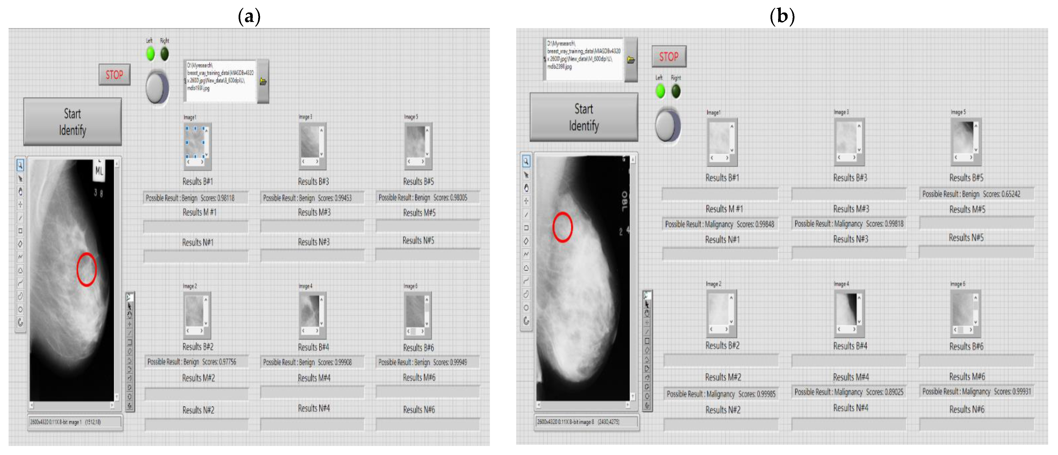
2.3. Human–Machine Interface Design for Breast Lesion Screening

As shown in Figure 3, LabVIEW 2019 Software (NI^TM), MATLAB Script tools, and open-source TensorFlow platform (Version 1.9.0) [41] were used to design a human–machine interface for breast lesion screening in automatic and manual operation modes to establish a CAD system. This human–machine interface integrated the following four functions:

(1)

ROI extraction function (manual or automatic modes): The path of mammography images can be set and images can be easily imported into the human–machine interface. In automatic screening mode, the most frequent region of breast tumors (based on the high distribution probability on right and left breasts) and the specific bounding box with 100 × 100 pixel dimension were used to automatically extract the feature maps (at least six maps) and save them in a designated file based on the screenshot sequence in automatic mode, or the clinician and radiologist can manually extract the feature maps. After the selection of the feature maps, they were saved in the designated file according to the sequence in manual mode.

(2)

Feature enhancement, noise removal, and feature extraction: three convolutional pooling layers (default structure) were used for digital image preprocessing and feature extraction.

(3)

Determination of kernel convolution window size and number: The size of kernel windows was set to 3 × 3 (default), the number of kernel windows to 16, and the size of MP window to 2 × 2. After the convolution processes in each convolutional layer, the same number of MP processes were performed. The size and number of kernel convolution windows can be set by the users (clinicians and radiologists).

(4)

Pattern recognition function: the open-source TensorFlow platform [41] was used to carry out an MCNN-based classification with a suitable number of convolution layers and kernel windows.

In the proposed human–machine interface, the clinicians and radiologists can change between automatic and manual screening modes (Figure 3a and Figure 3b, respectively). For example, clinicians and radiologists can manually select six ROIs, capture screenshots (default six feature maps), and save these screenshots in a designated file by sequence order. Then, the classifier performs an automatic recognition task based on the priority sequence order and returns the classification results. Thus, clinicians can confirm the possible breast lesion sites and identify their classes.

3. Experimental Results

The MIAS image database consists of four sizes of mammography images of which most have sizes of 4320 pixels × 2600 pixels [30,31,32]. Hence, this study used this size for the image collection of training and testing datasets for the f breast lesions screening. Each image had a vertical and horizontal resolution of 600 dpi and 24-bit depth. There were 78 subjects (156 mammography images in total of the left and right breasts, including 62 abnormality images (malignant or benign tumor images) and 94 normality images (tumor-free images)). The clinical information was confirmed and agreed upon by expert radiologists for biomarkers, such as image size, image category, background tissue, class of abnormality, and severity of abnormality [30,31]. The manual operation mode was selected by using the proposed human–machine interface and biomarker information was used as a reference to select screenshots within the ROI in 156 images, which included 422 tumor images and 578 tumor-free images (a total of 1000 images). At the training stage, 211 screenshots containing breast lesion images and 289 normal screenshots were randomly selected, respectively, and then the ADAM optimization algorithm was used to train the MCNN-based classifier by adjusting the classifier’s network parameters with the modulated weights and learning rates. The remaining 50% of images were used to test the classifier’s recognition capability in the recalling stage. In this study, the two models of MCNN-based classifiers (Model #1 and Model #2) were shown in

Table 3. Different convolutional pooling layer models for feature enhancement and extraction (Models #1–#2).

Model	1st Convolutional Window and Window Size	2nd Convolutional Window and Window Size	3rd Convolutional Window and Window Size	Stride/Padding	Maximum Pooling Window	Stride
1	Fractional Order, 3 × 3, 2	Kernel, 3 × 3, 16	Kernel, 3 × 3, 16	1/1	2 × 2, 16	2
2	Kernel, 3 × 3, 16	Kernel, 3 × 3, 16	Kernel, 3 × 3, 16	1/1	2 × 2, 16	2

, which were used to establish an image processing layer, consisting of three convolutional pooling layers. In Model #1, the first convolutional layer was set by using two 3 × 3 fractional-order (with fractional-order parameter = 0.30) convolution windows for 2D spatial convolutional processes. There were 16 kernel convolutional processes in the second and third layers with 3 × 3 kernel convolution windows to parallel produce the 16 feature maps. In this study, we implemented different MCNN-based classifiers in a multi-core personal computer-based platform (Intel^® Q370, Intel^® Core™ i7 8700, DDR4 2400 MHz 8 G*3) and also used the graphics processing unit (GPU) (NVIDIA^® GeForce^® RTX™ 2080 Ti, 1755 MHz, 11 GB GDDR6) to speed up the execution time for feature enhancement, feature extraction, and classification tasks. The classifiers’ algorithm was designed in the open-source TensorFlow platform (Version 1.9.0) [36].

During each convolutional process, each sliding window’s striding step was 1. To retain the feature map’s special characteristics after each convolutional process, we used the pooling process with padding = 1 and striding step = 2 to perform the MP process to reduce the dimension of the feature map. In Model #2, the three kernel convolution layers were set to sixteen 3 × 3 kernel convolution windows in parallel convolutional processes. As presented in Table 3, both models used three convolutional pooling layers for feature enhancement and extraction to gradually produce potential lesion contours. In the classification layer, the BPNN consisted of an input layer (with 625 input nodes), the 1st hidden layer (with 168 hidden nodes), the 2nd hidden layer (with 64 hidden nodes), and an output layer (with 2 output nodes). Then, the MCNN-based classifier used these enhanced feature maps to improve the classification accuracy. As shown in

Table 4. Cross-validation testing results for Model #1 and Model #2 (K_f = 10).

	Test Fold	1	2	3	4	5	6	7	8	9	10	Average Accuracy (%)
Model
1		96.14	97.43	98.07	97.96	98.93	98.07	96.35	95.60	96.89	98.28	97.37
2		97.00	96.60	95.40	96.20	97.60	94.40	95.00	98.10	96.00	95.00	95.93

, tenfold (K_f = 10) cross-validation was used to verify the proposed Model #2, and the accuracy (%) was used as an index to preliminarily evaluate the classification accuracy of the two models. The experimental results in Table 4 show that the three convolutional pooling layers + the fully connected BPNN had an average accuracy (%) of >95% for separating normality cases from abnormality ones. The average training times for Models #1 and #2 were <280 and <310 s CPU time, respectively. Therefore, with Model #2, exactly 1000 training epochs were used to train the classifier. Figure 4a shows the classifier’s performance validation including the classification accuracy versus the training epoch. Figure 4b reveals the training efficiency as the training convergence curve (with loss function) versus the training epoch, where the blue solid line represents the training performance test, and the orange solid line denotes the classification performance validation. As the number of training epochs increased so did the classification accuracy, which reached saturation after 400 training epochs. Finally, the results of the training convergence curve converged, and the value of the loss function was minimized (reached the convergence condition). The two models presented promising results for breast lesion screening. However, the fractional-order convolutional window for Model #1’s first layer required the selection of appropriate fractional-order parameters to achieve better image processing results. Therefore, the architecture of Model #2 was used to carry out a multilayer MCNN-based classification in this study. Figure 5 indicates the visualizable confusion matrix of the multilayer classifier based on Model #2, in which 500 untrained feature maps were used for lesion screening. The experimental results showed that the four element values comprised 203 TPs, 8 FPs, 282 TNs, and 7 FNs for the identification of normality and abnormality, and they were used to calculate the four evaluation indexes, including precision (%), recall (%), accuracy (%), and F1 score, to further evaluate the classifier’s predictive performances.

Based on the aforementioned tests, Model #2 was selected in this study as the basis architecture to construct four types of multilayer classifiers, including from Model #2-1 to Model #2-4. The number of kernel convolutional windows in the three convolutional pooling layers was set to 4, 8, 16, and 32 [36], respectively, as seen in

Table 5. Different numbers of the kernel convolutional window for Model #2.

Model	1st Convolutional Window and Window Size	2nd Convolutional Window and Window Size	3rd Convolutional Window and Window Size	Stride/Padding	Maximum Pooling Window	Stride
2-1	Kernel, 3 × 3, 4	Kernel, 3 × 3, 4	Kernel, 3 × 3, 4	1/1	2 × 2, 4, 8, 16, 32	2
2-2	Kernel, 3 × 3, 8	Kernel, 3 × 3, 8	Kernel, 3 × 3, 8	1/1		2
2-3	Kernel, 3 × 3, 16	Kernel, 3 × 3, 16	Kernel, 3 × 3, 16	1/1		2
2-4	Kernel, 3 × 3, 32	Kernel, 3 × 3, 32	Kernel, 3 × 3, 32	1/1		2

. Each time, half of the dataset was used to train the classifier and the other half of those was used to validate the classifier’s performance with the four different multilayer structures. Then, the 10-fold cross-validation method was used to validate the classifier’s performances. Each testing fold could obtain the TP, FP, TN, and FN from the outcomes of the confusion matrix, as shown in Figure 5. Equations (1)–(4), were used to compute the four indexes, as precision (%), recall (%), accuracy (%), and F1 score.

Table 6. Experimental results of k-fold cross-validation (K_f = 10) for Model #2-1 to Model #2-4 with different numbers of kernel. Convolutional windows (3 × 3, 4, 8, 16, and 32) and MP windows (2 × 2, 4, 8, 16, and 32) in three convolutional pooling layers.

Model	Average Precision (%)	Average Recall (%)	Average Accuracy (%)	Average F1 Score	Average CPU Time (s) for Training
2-1	92.03	88.94	91.57	0.9076	148.02
2-2	94.77	92.81	95.03	0.9389	237.39
2-3	95.19	95.19	95.04	0.9516	308.38
2-4	94.06	93.60	95.30	0.9395	332.05

showed the testing results with changing the different number of kernel convolutional windows. In clinical testing, precision (%) and recall (%) are the primary indexes for evaluating the classification capability, in addition to accuracy (%). Precision (%) represented the accuracy of the predicted TPs (actual abnormality), whereas recall (%) represented the accuracy of the actual TPs. The two evaluation indexes were both higher than 80.0%, indicating that the classifier had a promising recognition capacity. Recall (%) was TP-detected rate as the positive predictive value (PPV) in the tested dataset. Usually, the PPV index, >80.0%, indicated that the classifier had good prediction performance. The 10-fold cross-validation results demonstrated that the results of average precision (%) and average recall (%) of Model #2-3 were better than the other three models (Model #2-1, Model #2-2, and Model #2-4). The F1 score was also an evaluation index that fused the indicators of precision (%) and recall (%), and an F1 score of >0.9000 indicated that the classifier model was satisfactory for the recognition capacity. As seen in the experimental results in Table 6 (as seen in the previous study of [36]), the F1 scores of all the four models were >0.9000. The average F1 score of Model #2-3 was superior to the other three models. The average accuracy (%) of Model #2-4 (95.30%) was greater than Model #2-3 (95.04%). However, the 10-fold cross-validation results indicated that Model #2-4 had too many kernel convolutional windows and would produce a large number of feature parameters, which affected the learning capacity of Model #2-4, resulting in a higher generalization error and poor generalization capacity. Too many kernel convolutional windows would decay the learning and generalization capacity in the multilayer structure, resulted in affecting the overall classifier’s performance. Based on the experimental results in Table 4 and Table 6, as seen in four evaluation indexes and training time (as seen in Figure 5), this study we suggested the following:

• The suitable classifier structure consisted of three convolutional pooling layers and a fully connected BPNN was suggested to establish the multilayer classifier model;
• The size of the kernel convolution window could be set to 3 × 3 for convolutional operations;
• The better capacity of feature extraction could be achieved by using 16 kernel convolution windows and 16 MP winds for each convolutional pooling layer, which could increase the classifier’s recognition capability.

Based on the architecture of three convolutional pooling layers, the model of 2D spatial and 1D CNN [42] was also used to establish four types of multilayer classifiers, including from Model #3-1 to Model #3-4, as seen in the model summary in

Table 7. Summary of models for the 2D spatial and 1D CNN-based classifier (Model #3-1 to Model #3-4).

Model	First Convolutional Pooling Layer	Second Convolutional Pooling Layer	Third Convolutional Pooling Layer	Classification Layer	Average Training Time (s)	Average Accuracy (%)
3-1	2D Kernel Convolutional Process, 3 × 3, 8 (Stride = 1) Maximum Pooling, 2 × 2, 8 (Stride = 2)	Flattening Process 1D Kernel Convolutional Process, 1 × 100, 8	1D Kernel Convolutional Process, 1 × 100, 8 1D Pooling Processes (Stride = 10)	BPNN: Input Layer (250 nodes), 1st Hidden Layer (64 nodes), 2nd Hidden Layer (64 nodes), and Output Layer (2 nodes)	322.74 (Loss = 0.1211)	93.40
3-2		Flattening Process 1D Kernel Convolutional Process, 1 × 100, 8 1D Pooling Processes (Stride = 10)	-		305.39 (Loss = 0.1650)	94.00
3-3	2D Kernel Convolutional Process, 3 × 3, 4 (Stride = 1) Maximum Pooling, 2 × 2, 4 (Stride = 2)	Flattening Process 1D Kernel Convolutional Process, 1 × 100, 4	1D Kernel Convolutional Process, 1 × 100, 4 1D Pooling Processes (Stride = 10)		347.67 (Loss = 0.2293)	91.20
3-4		Flattening Process 1D Kernel Convolutional Process, 1 × 100, 4 1D Pooling Processes (Stride = 10)	-		324.27 (Loss = 0.1538)	94.80

. The four models algorithm was implemented in the open-source TensorFlow platform (Version 1.9.0) [36]. The number of kernel convolutional windows in the convolutional pooling layers was set to 8 for Model #3-1 and Model #3-2 and was set to 4 for Model #3-3 and Model #3-4, respectively. Hence, we could construct the multilayer classifiers, consisting of a 2D kernel convolutional pooling layer (with stride = 1 for convolutional processes and stride = 2 for MP processes), flattening layer, one- or two-round 1D kernel convolutional pooling layers, and a fully connecting classification network (Classification Layer). In the 2nd and 3rd convolutional layers, the 1D kernel convolutional processes used the discrete Gaussian function (with stride = 1) with 100 data lengths of the convolutional window to extract the 1D feature vector. In the 1D pooling layer, the dimension of the feature signal was reduced from 1 × 2500 to 1 × 250 (with stride = 10). In the classification layer, the BPNN consisted of an input layer (with 250 input nodes), 1st hidden layer (with 64 hidden nodes), 2nd hidden layer (with 64 hidden nodes), and an output layer (with 2 output nodes). Each classifier could identify the normality (disease absent) and abnormality (disease present). The ADAM optimization algorithm was also used to adjust the network connecting parameters by using iterative computations. With the same dataset (trained and untrained datasets) and 10-fold cross-validation tests, the models with two convolutional pooling layers (Model #3-2 and Model #3-4) had higher average accuracy than those with three convolutional pooling layers (Model #3-1 and Model #3-3). Model #3-2 took an average CPU time of 305.39 s for training the classifier to identify the breast lesions, and the average CPU time was less than the other three models. Based on the experimental results as shown in Table 7, it could be seen that the 2D spatial and 1D CNN-based classifier also had promising performances in the design cycle, recognition capability, network parameters adjustment (iteration computations), and computational time. Hence, we suggested the use of Model #3-2-based classifier to apply in clinical applications.

In addition, we randomly fed three groups of trained datasets, including 100 tumor-free images, 50 B tumor images, and 50 M tumor images to train the same structure of classifier, which consisted of three convolutional pooling layers and a fully connected BPNN with three outputs for the identified three classes. The ADAM algorithm was also used to adjust the classifier’s network parameters, which required 104.02 s CPU time to achieve the convergence condition. After training the classifier (as seen in Figure 6), with the randomly selected 200 untrained datasets (100 Nor tissues, 50 B, and 50 M tumors), the confusion matrix showed the nine element values, including 90 TPs (40 B and 50 M tumors), 10 FPs, 96 TNs, and 4 FNs, for the identified tumor-free and tumor images, which were used to calculate the four evaluation indexes, such as precision (%) = 96.15 (%), recall (%) = 90.90%, accuracy (%) = 93.00%, and F1 score = 0.9278. The above criteria can be used to validate the classifier’s pattern recognition capacity for the identified three classes (Nor, B tumor, and M tumor).

4. Discussion

The DL-based classifier with multiconvolutional pooling processes could perform the end-to-end image/signal enhancement, noise filtering, feature extraction, and classification tasks, including 2D CNN, 1D CNN, and combining 2D spatial and 1D CNN models, which could provide in clinical/medical applications, such as image (mammography, chest X-ray, computed tomography) [36,42,43,44]/signal (electrocardiogram (ECG), heart sound, voice, and speech) classification [45,46,47,48,49], image segmentation [4,50], and pathological characteristics detection [51], as seen in

Table 8. DL-based classifiers for applications, including image/signal classification, image segmentation, and pathological characteristics detection.

Literature	Database	Method	Purpose
[42]	MIAS Image Database [30,31]	2D spatial and 1D CNN	Breast Lesions Screening Precision: 96.70%; Recall: 96.13%; Accuracy: 96.40%; F1 Score: 0.9641
[43]	CBIS-DDSM Database [20]	Dense-Unet Model	Calcification Detection Sensitivity: 91.22%; Specificity: 92.01%; Accuracy: 91.47%; F1 Score: 0.9219
[44]	Collected by Department of Breast and Endocrine Surgery at Hallym University Sacred Heart Hospital [44]	DenseNet-169, EfficientNet-B5	Automated Breast Cancer Detection (1) DenseNet-169: AUC = 0.952 ± 0.005; Mean Sensitivity: 87.0%; Mean Specificity: 88.4%; Mean Accuracy: 88.1% (2) EfficientNet-B5: AUC = 0.954 ± 0.020; Mean Sensitivity: 88.3%; Mean Specificity: 87.9%; Mean Accuracy: 87.9%
[4]	E-Da Hospital Image Database [4]	DNN (Deep Neural Network)	BI-RADS Classification Sensitivity: 95.31%; Specificity: 99.15%; Accuracy: 94.22% [49]
[11]	DDSM Database [19]	Attention Dense-Unet Model	Mass Segmentation Sensitivity: 77.89%; Specificity: 84.69%; Accuracy: 78.38%
[45]	MIT-BIH Arrhythmia Dataset [53]	11-layer 1D CNN (DNN)	Arrhythmia Detection Precision: 75.91%; Recall: 92.88%; Accuracy: 95.85%; F1 Score: 0.8115
[46]	MIT-BIH Arrhythmia Dataset [53]	11-layer 2D CNN (DNN)	Arrhythmia Detection Precision: 89.31%; Recall: 91.69%; Accuracy: 89.31%; F1 Score: 0.8957
[48]	8732 Urban Sounds (Ten Classes) [48]	1D CNN (DNN) 3, 5, and 10-Convolution Cross-Validation	Environmental Sound Classification Average Accuracy: 94.46%
[49]	Uzbek Dataset Consists of 207 h of Transcribed Audio Spoken by 1281 Speakers [49]	Deep Neural Network Hidden Markov Model (DNN-HMM)	Automatic Speech Recognition for Uzbek Language Training Accuracy: 96% Testing Accuracy: 93%
[50]	Audio and Video: AVEC2013 and AVEC2014 Database [50]	1D CNN and 2D CNN	Depression Recognition RMSE 7–10 MAE: 5–9

. In image classification [42,43,44] and image segmentation [4,50], with the DDSM (Digital Database of Screening Mammography Database) [19], CBIS (Curated Breast Imaging Subset of Digital Database for Screening Mammography)-DDSM Database [20], MIAS Image Database [30,31], and Hospital Image Database [4,44], the DL-based methods, such as 2D spatial and 1D CNN [42], Dense-Unet model [43], DenseNet-169 and EfficientNet-B5 [44], DNN [4], and Attention Dense-Unet, and Dense-Unet models, had multiconvolutional pooling layers and a fully connected classification network to carry out a classifier model for medical purposes in breast lesions (cancer) screening, calcification detection, and mass segmentation. For example, the authors of [44] proposed that DenseNet-169 and EfficientNet-B5 models could highlight ROI with the Grad-CAM (Gradient-Weighted Class Activation Mapping) processes [51] to indicate the positive region in the red color-coded areas for detected malignant lesions. In both craniocaudal and mediolateral oblique view images, the visualization manner could easily locate the mass or calcification. DenseNet-169 and EfficientNet-B5 had mean accuracy rates of 88.1% (mean sensitivity: 87.0%, mean specificity: 88.4%) and 87.9% (mean sensitivity: 88.3%, mean specificity: 87.9%) for automated breast cancer detection, respectively. Literature [42] proposed a 2D spatial and 1D CNN-based classifier for breast lesions screening. Based on three convolutional pooling layers, in the first layer, the possible breast lesions’ 2D spatial and edge information could be enhanced by integral image (II)-based convolutional process [42,52]; in the second and third layers, two-round 1D convolutional processes and 1D pooling process could filter the noise and extract the stable 1D feature parameters for quantifying the different levels in order to separate the normal (Nor) from the abnormality (B and M classes). Hence, this pattern recognition scheme could reduce the dimension of feature parameters and did not require the complex computational processes to perform the classification task. In addition, the classification accuracy could be depended to an average precision of 96.70%, average recall of 96.13%, average accuracy of 96.40%, and average F1 score of 0.9641 for identified the breast lesions.

In digital signal classification, for example, with the MIT (Massachusetts Institute of Technology)–BIH (Beth Israel Hospital Arrhythmia Laboratory) Arrhythmia Dataset [53], after data preprocessing using the Butterworth filter, 11-layer 1D CNN [45] and 11-layer 2D CNN-based [46] classifiers were used to deal with the ECG signals and achieved average accuracies of 95.85% and 89.31% on arrhythmia classification (12 rhythm classes), respectively. The 2D CNN-based classifier outperformed the 1D CNN-based classifier in terms of F1 score (2D CNN’s F1: 0.8957, 1D CNN’s F1 score: 0.8115). It could be seen that there was a good balance between the precision (%) and the recall (%) scores. However, the accuracy of the 2D CNN model affected the classifier’s effectiveness for application in 1D signal classification. In sound classification, with the 3, 5, and 10-convolution cross-validation tests, the 1D CNN-based classifier also had a higher average accuracy of 94.00% on ten classes of urban sounds. Different durations of environmental sounds might occur, thus frame (window) length and sampling rate would affect the signal resolution for analyzing and quantizing frequencies. Hence, applying a variable width window in audio signal acquisition would overcome the above restriction [48]. In automatic speech recognition (ASR), literature [49] proposed the deep neural network hidden Markov model (DNN-HMM) to carry out an ASR system for the Uzbek language. With the Uzbek Language Dataset (1281 speakers [49]), the DNN-HMM-based classifier had 96% training accuracy and 93% testing accuracy with a word error rate of 14.3% for ASR applications. In pathological characteristics detection, literature [51] reviewed DL-based methods to extract a representation of depression from the audio and video database for automatic depression recognition (ADR), which were evaluated on the AVEC2013 and AVEC2014 databases [11], the range 7–10 of RMSE (root mean square error), and range 5–9 of MAE (mean absolute error) could evaluate the classifier’s performance for ADR application. After reviewing the above literature, we could suggest the following:

• based on three convolutional pooling layers, in the first layer, the fractional-order convolutional process [35,36], Grad-CAM Process [44,51], and II-based convolutional process [42,52] could enhance the 2D spatial and edge information to easily locate ROI and extract the feature patterns;
• in the second and third layers, two-round 2D convolutional pooling processes or 1D convolutional pooling processes [35,36,42];
• these processes were continuously to perform the end-to-end noise filtering and feature extraction tasks, which could extract the high-level spatial information, such as the possible lesion’s contour and shape, to detect nonlinear features representation and increase the classification accuracy;
• reducing the number of convolution layers and convolution kernel and pooling processes could reduce the dimension of feature parameters and also reduce the computational complexity and computational time;
• in the classification layer, the ADAM algorithm [39,40] or straightforward mathematical algorithm without iteration computations [42] could be used to adjust the BPNN’s network-connected parameters and achieve promising training accuracy.

5. Conclusions

Breast tumors can be divided into four stages based on the tumor size and the degree of lymph node metastasis. The early discovery of abnormalities will not only improve the survival rates but also lead to better therapeutic efficacy. In addition, early signs of breast lesions can be detected, and statistics showed that early detection can increase survival rates by more than 90%. In general, periodic self-examinations or breast radiologic examinations, including mammography, breast-computed tomography, breast ultrasound, and breast magnetic resonance imaging, can be conducted for further testing [54,55,56]. Mammography and breast ultrasound are the first-line detection methods. Breast ultrasound has a lower detection capacity for small calcifications and should be used in conjunction with mammography to evaluate suspected lesions. Conventional B-mode ultrasound can only identify potential tumor sites; ultrasound elastography [43] can be used to further confirm the characteristics of suspected mass regions. In this study, mammography was used for the rapid screening of breast lesions. A multilayer classifier was designed for this medical purpose, and the number of convolution layers and the number and size of kernel convolutional windows were determined using cross-validation methods. After tenfold cross-validation, the multilayer model with the three convolutional pooling layers and a fully connected BPNN was suggested to carry out classification, and the classifier based on this model showed promising feature extraction and classification accuracy for the identified two classes (normality and abnormality or Nor, B, and M). The pattern recognition scheme used in this study can be used to determine the presence/absence of tumors and tumor classes. We believe that classification performance can be improved in the future to determine whether a tumor is B or M by continuously adding new clinical image datasets. Fine-needle aspiration, core-needle biopsy, or tissue-section tests must be performed by a physician or the pathology department staff to obtain definitive results on the nature of a mass. Our model can also be used by physicians as a diagnostic tool to obtain a good reference for diagnosis.

References

1. World Cancer Day 2021: Spotlight on IARC Research Related to Breast Cancer. 2021. Available online: https://www.iarc.who.int/featured-news/world-cancer-day-2021/ (accessed on 12 July 2022).
2. Ministry Health and Welfare, Taiwan, 2020 Cause of Death Statistics. 2021. Available online: https://dep.mohw.gov.tw/dos/lp-1800-113.html (accessed on 12 July 2022).
3. IARC Working Group on the Evaluation of Cancer-Preventive Interventions, Breast Cancer Screening. In IARC Handbooks of Cancer Prevention; International Agency for Research on Cancer: Lyon, France, 2016; Volume 15.
4. Tsai, K.-J.; Chou, M.-C.; Li, H.-M.; Liu, S.-T.; Hsu, J.-H.; Yeh, W.-C.; Hung, C.-M.; Yeh, C.-Y.; Hwang, S.-H. A high-performance deep neural network model for BI-RADS classification of screening mammography. Sensors 2022, 22, 1160. [Google Scholar] [CrossRef] [PubMed]
5. Morris, E.A.; Comstock, C.E.; Lee, C.H. ACR BIRADS® magnetic resonance imaging. In ACR BI-RADS® Atlas, BREAST Imaging Reporting and Data System; American College of Radiology: Reston, VA, USA, 2013. [Google Scholar]
6. Sickles, E.; d’Orsi, C.; Bassett, L.; Appleton, C.; Berg, W.; Burnside, E.; Feig, S.; Gavenonis, S.; Newell, M.; Trinh, M. Acr bi-rads® mammogramphy. ACR BI-RADS® Atlas Breast Imaging Report. Data Syst. 2013, 5, 2013. [Google Scholar]
7. Breast Imaging-Reporting and Data System (BI-RADS). Available online: https://radiopaedia.org/articles/breast-imagingreporting-and-data-sytem-bi-rads (accessed on 20 July 2021).
8. Halkiotis, S.; Botsis, T.; Rangoussi, M. Automatic detection of clustered microcalcifications in digital mammograms using mathematical morphology and neural networks. Signal Process. 2007, 87, 1559–1568. [Google Scholar] [CrossRef]
9. Mahersia, H.; Boulehmi, H.; Hamrouni, K. Development of intelligent systems based on Bayesian regularization network and neuro-fuzzy models for mass detection in mammograms: A comparative analysis. Comput. Methods Programs Biomed. 2016, 126, 46–62. [Google Scholar] [CrossRef]
10. Vijayarajeswari, R.; Parthasarathy, P.; Vivekanandan, S.; Basha, A.A. Classification of mammogram for early detection of breast cancer using SVM classifier and Hough transform. Measurement 2019, 146, 800–805. [Google Scholar] [CrossRef]
11. He, L.; Niu, M.; Tiwari, P.; Marttinen, P.; Su, R.; Jiang, J.; Guo, C.; Wang, H.; Ding, S.; Wang, Z.; et al. Deep learning for depression recognition with audiovisual cues: A review. Inf. Fusion 2022, 80, 56–86. [Google Scholar] [CrossRef]
12. Sathyan, A.; Martis, D.; Cohen, K. Mass and calcification detection from digital mammogramsusing UNets. In Proceedings of the 2020 7th IEEE International Conference on Soft Computing & Machine Intelligence (ISCMI), Stockholm, Sweden, 14–15 November 2020; pp. 229–232. [Google Scholar]
13. Agarwal, R.; Díaz, O.; Yap, M.H.; Lladó, X.; Martí, R. Deep learning for mass detection in full field digital mammograms. Comput. Biol. Med. 2020, 121, 103774. [Google Scholar] [CrossRef]
14. Xu, S.; Adeli, E.; Cheng, J.Z.; Xiang, L.; Li, Y.; Lee, S.W.; Shen, D. Mammographic mass segmentation using multichannel and multiscale fully convolutional networks. Int. J. Imaging Syst. Technol. 2020, 30, 1095–1107. [Google Scholar] [CrossRef]
15. Shelhamer, E.; Long, J.; Darrell, T. Fully convolutional networks for semantic segmentation. IEEE Trans. Pattern Anal. Mach. Intell. 2017, 39, 640–651. [Google Scholar] [CrossRef]
16. Lee, J.; Nishikawa, R.M. Automated mammographic breast density estimation using a fully convolutional network. Med. Phys. 2018, 45, 1178–1190. [Google Scholar] [CrossRef]
17. Ben-Ari, R.; Akselrod-Ballin, A.; Karlinsky, L.; Hashoul, S. Domain specific convolutional neural nets for detection of architectural distortion in mammograms. In Proceedings of the 2017 IEEE 14th International Symposium on Biomedical Imaging, Melbourne, Australia, 18–21 April 2017; pp. 552–556. [Google Scholar]
18. Bruno, A.; Ardizzone, E.; Vitabile, S.; Midiri, M. A novel solution based on scale invariant feature transform descriptors and deep learning for the detection of suspicious regions in mammogram images. J. Med. Signals Sens. 2020, 10, 158–173. [Google Scholar] [PubMed]
19. Heath, M.; Bowyer, K.; Kopans, D.; Kegelmeyer, P.; Moore, R.; Chang, K.; Munishkumaran, S. Current status of the digital database for screening mammography. In Digital Mammography; Springer: Dordrecht, The Netherlands, 1998; pp. 457–460. [Google Scholar]
20. Lee, R.S.; Gimenez, F.; Hoogi, A.; Miyake, K.K.; Gorovoy, M.; Rubin, D.L. A curated mammography data set for use in computer-aided detection and diagnosis research. Sci. Data 2017, 4, 170177. [Google Scholar] [CrossRef] [PubMed]
21. Samala, R.K.; Chan, H.; Hadjiiski, L.; Helvie, M.A.; Richter, C.D.; Cha, K.H. Breast cancer diagnosis in digital breast tomosynthesis: Effects of training sample size on multi-stage transfer learning using deep neuralnets. IEEE Trans. Med. Imaging 2019, 38, 686–696. [Google Scholar] [CrossRef]
22. Valkonen, M.; Isola, J.; Ylinen, O.; Muhonen, V.; Saxlin, A.; Tolonen, T.; Nykter, M.; Ruusuvuori, P. Cytokeratin-supervised deep learning for automatic recognition of epithelial cells in breast cancers stained for ER, PR, and Ki-67. IEEE Trans. Med. Imaging 2020, 39, 534–542. [Google Scholar] [CrossRef] [PubMed]
23. Lee, S.; Kim, H.; Higuchi, H.; Ishikawa, M. Classification of metastatic breast cancer cell using deep learning approach. In Proceedings of the 2021 International Conference on Artificial Intelligence in Information and Communication (ICAIIC), Jeju Island, Korea, 20–23 April 2021; pp. 425–428. [Google Scholar]
24. Thanh, D.N.H.; Kalavathi, P.; Thanh, l.; Prasath, V.B.S. Chest X-ray image denoising using Nesterov optimization method with total variation regularization. Procedia Comput. Sci. 2020, 171, 1961–1969. [Google Scholar] [CrossRef]
25. Gu, J.; Wang, Z.; Kuen, J.; Ma, L.; Shahroudy, A.; Shuai, B.; Liu, T.; Wang, X.; Wang, G.; Cai, J.; et al. Recent advances in convolutional neural network. Pattern Recognit. 2018, 77, 354–377. [Google Scholar] [CrossRef]
26. Kiranyaz, S.; Avci, O.; Abdeljaber, O.; Ince, T.; Gabbouj, M.; Inman, D.J. 1D convolutional neural networks and applications: A survey. Mech. Syst. Signal Processing 2021, 151, 107398. [Google Scholar] [CrossRef]
27. Chansong, D.; Supratid, S. Impacts of Kernel size on different resized images in object recognition based on convolutional neural network. In Proceedings of the 2021 9th International Electrical Engineering Congress (iEECON), Pattaya, Thailand, 10–12 March 2021. [Google Scholar]
28. Wu, J.; Chen, P.; Li, C.; Kuo, Y.; Pai, N.; Lin, C. Multilayer fractional-order machine vision classifier for rapid typical lung diseases screening on digital chest X-Ray images. IEEE Access 2020, 8, 105886–105902. [Google Scholar] [CrossRef]
29. Lin, C.; Wu, J.; Li, C.; Chen, P.; Pai, N.; Kuo, Y. Enhancement of chest X-ray images to improve screening accuracy rate using iterated function system and multilayer fractional-order machine learning classifier. IEEE Photonics J. 2020, 12, 1–19. [Google Scholar] [CrossRef]
30. Pilot European Image Processing Archive, The Mini-MIAS Database of Mammograms. 2012. Available online: http://peipa.essex.ac.uk/pix/mias/ (accessed on 12 July 2022).
31. Mammographic Image Analysis Society (MIAS) Database v1.21. 2019. Available online: https://www.repository.cam.ac.uk/handle/1810/250394 (accessed on 12 July 2022).
32. Oza, P.; Sharma, P.; Patel, S.; Bruno, A. A bottom-up review of image analysis methods for suspicious region detection in mammograms. J. Imaging 2021, 7, 190. [Google Scholar] [CrossRef]
33. Chicco, D.; Jurman, G. The advantages of the Matthews correlation coefficient (MCC) over F1 score and accuracy in binary classification evaluation. BMC Genom. 2020, 21, 6. [Google Scholar] [CrossRef] [PubMed] [Green Version]
34. LeCun, Y.; Bengio, Y.; Haffner, P. Gradient-based learning applied to document recognition. Proc. IEEE 1998, 86, 2278–2324. [Google Scholar] [CrossRef]
35. Zhang, X. A Convolutional Neural Network Assisted Fast Tumor Screening System Based on Fractional-Order Image Enhancement: The Case of Breast X-ray Medical Imaging. Master’s Thesis, Department of Electrical Engineering, National Chin-Yi University of Technology, Taichung, Taiwan, 2021. [Google Scholar]
36. Chen, P.; Zhang, X.; Wu, J.; Pai, C.C.; Hsu, J.; Lin, C.; Pai, N. Automatic breast tumor screening of mammographic images with optimal convolutional neural network. Appl. Sci. 2022, 12, 4079. [Google Scholar] [CrossRef]
37. Chougrad, H.; Zouaki, H.; Alheyane, O. Deep convolutional neural networks for breast cancer screening. Comput. Methods Programs Biomed. 2018, 157, 19–30. [Google Scholar] [CrossRef] [PubMed]
38. Ho, Y.; Wookey, S. The real-world-weight cross-entropy loss function: Modeling the costs of mislabeling. IEEE Access 2019, 8, 4806–4813. [Google Scholar] [CrossRef]
39. Kingma, D.P.; Ba, J. Adam: A method for stochastic optimization. In Proceedings of the 3rd International Conference for Learning Representations, San Diego, CA, USA, 7–9 May 2015. [Google Scholar]
40. Ma, J.; Yarats, D. Quasi-hyperbolic momentum and Adam for deep learning. Proc. ICLR 2019, 2019, 1–38. [Google Scholar]
41. Li, Y.; Shen, T.; Chen, C.; Chang, W.; Lee, P.; Huang, C.-C. Automatic detection of atherosclerotic plaque and calcification from intravascular ultrasound Images by using deep convolutional neural networks. IEEE Trans. Ultrason. Ferroelectr. Freq. Control 2021, 68, 1762–1772. [Google Scholar] [CrossRef]
42. Lin, C.; Lai, H.; Chen, P.; Wu, J.; Pai, C.; Su, C.; Ho, H.-W. Breast lesions screening of mammographic images with 2D spatial and 1D convolutional neural network-based classifier. Appl. Sci. 2022, 12, 7516. [Google Scholar] [CrossRef]
43. AlGhamdi; Abdel-Mottaleb, M.; Collado-Mesa, F. Du-net: Convolutional network for the detection of arterial calcifications in mammograms. IEEE Trans. Med. Imaging 2020, 39, 3240–3249. [Google Scholar] [CrossRef]
44. Suh, Y.J.; Jung, J.; Cho, B. Automated breast cancer detection in digital mammograms of various densities via deep learning. J. Pers. Med. 2020, 10, 211. [Google Scholar] [CrossRef]
45. Hannun, A.Y.; Rajpurkar, P.; Haghpanahi, M.; Tison, G.H.; Bourn, C.; Turakhia, M.P.; Ng, A.Y. Cardiologist-level arrhythmia detection and classification in ambulatory electrocardiograms using a deep neural network. Nat. Med. 2019, 25, 65–69. [Google Scholar] [CrossRef] [PubMed]
46. Kachuee, M.; Fazeli, S.; Sarrafzadeh, M. ECG heartbeat classification: A deep transferable representation. In Proceedings of the 2018 IEEE International Conference on Healthcare Informatics (ICHI), New York, NY, USA, 4–7 June 2018. [Google Scholar]
47. Mamatov, N.; Niyozmatova, N.; Samijonov, A. Software for preprocessing voice signals. Int. J. Appl. Sci. Eng. 2020, 18, 1–8. [Google Scholar]
48. Ragab, M.G.; Abdulkadir, S.J.; Aziz, N.; Alhussian, H.; Bala, A.; Alqushaibi, A. An ensemble one dimensional convolutional neural network with Bayesian optimization for environmental sound classification. Appl. Sci. 2021, 11, 4660. [Google Scholar] [CrossRef]
49. Mukhamadiyev, A.; Khujayarov, I.; Djuraev, O.; Cho, J. Automatic speech recognition method based on deep learning approaches for Uzbek language. Sensors 2022, 22, 3683. [Google Scholar] [CrossRef]
50. Li, S.; Dong, M.; Du, G.; Mu, X. Attention dense-u-net for automatic breast mass segmentation in digital mammogram. IEEE Access 2019, 7, 59037–59047. [Google Scholar] [CrossRef]
51. Selvaraju, R.R.; Cogswell, M.; Das, A.; Vedantam, R.; Parikh, D.; Batra, D. Grad-CAM: Visual explanations from deep networks via gradient-based localization. In Proceedings of the 2017 IEEE International Conference on Computer Vision (ICCV), Venice, Italy, 22–29 October 2017. [Google Scholar]
52. Ehsan, S.; Clark, A.F.; Rehman, N.; McDonald-Maier, K.D. Integral images: Efficient algorithms for their Computation and storage in resource-constrained embedded vision systems. Sensors 2015, 15, 16804–16830. [Google Scholar] [CrossRef]
53. George Moody and Roger Mark, MIT-BIH Arrhythmia Database. 2005. Version: 1.0.0. Available online: https://physionet.org/content/mitdb/1.0.0/ (accessed on 12 July 2022).
54. Makeev, A.; Glick, S.J. Low-Dose contrast-enhanced breast CT using spectral shaping filters: An experimental study. IEEE Trans. Med. Image 2017, 36, 2417–2423. [Google Scholar] [CrossRef]
55. Wu, J.; Chen, P.; Lin, C.; Chen, S.; Shung, K.K. Breast benign and malignant tumors rapidly screening by ARFI-VTI elastography and random decision forests based classifier. IEEE Access 2020, 8, 54019–54034. [Google Scholar] [CrossRef]
56. Gubern-M’erida, A.; Kallenberg, M.; Mann, R.M.; Martí, R.; Karssemeijer, N. Breast segmentation and density estimation in breast MRI: A fully automatic framework. IEEE J. Biomed. Health Inform. 2015, 19, 349–357. [Google Scholar] [CrossRef]
Figure 1. Feature patterns (100 × 100 pixels) of Nor, B, and M. (a) Templates of B tumors; (b) templates of M tumors; (c) templates of Nor feature patterns.
Processes 10 01867 g001
Figure 2. Architecture of multilayer convolutional neural network (MCNN)-based classifier for breast lesion screening.
Processes 10 01867 g002
Figure 3. Human–machine interface of breast lesion screening operation. (a) Automatic screening mode for malignant or benign tumor as red circle; (b) manual screening mode.
Processes 10 01867 g003
Figure 4. Training history curves of the trained MCNN-based classifier. (a) Classification performance validation observed in the classification accuracy versus training epoch; (b) training efficient observed in the training convergence curve versus training epoch.
Processes 10 01867 g004
Figure 5. Output confusion matrix of the multilayer classifier based on Model #2 for identifying the normality and abnormality.
Processes 10 01867 g005
Figure 6. Output confusion matrix of the multilayer classifier for identification of the Nor, B, and M tumor classes.
Processes 10 01867 g006