Stochastic Optimization Operation of the Integrated Energy System Based on a Novel Scenario Generation Method

Abstract

The application of integrated energy systems is significant for realizing the comprehensive utilization of various energy sources and improving the utilization rate of renewable energy. At present, the optimal operation of integrated energy systems is a research hotspot. However, shortcomings remain in the stochastic optimization operation and the scenario generation method. This paper proposes a stochastic optimization operation model of an integrated energy microgrid based on an advanced multi-scenario generation method. First, this paper establishes the time-divided probability distribution model of the forecasting error of the uncertain factors, such as photovoltaic (PV) power and load, which provide the basis for generating scenarios. Moreover, the covariance matrix is used to calculate the time correlation of the time-divided probabilistic distributed models, and the parameters of the covariance matrix are optimized. Second, based on multiple typical scenarios, the stochastic optimization operation model of the integrated energy microgrid is established. Finally, the real data is used to verify the proposed method. The results show that the nonparametric kernel density estimation method has the best fitting effect. On this basis, the time correlation and the operation costs are compared with the scenario sets generated by other methods, which proves the advantages of the proposed multi-scenario generation method and stochastic optimization operation model.

1. Introduction

With rising energy demands and increasing concerns about environmental problems, seeking alternative energy, reducing the use of fossil energy, and improving energy utilization efficiency have become inevitable choices for the development of human society. Renewable energy power generation has many advantages and can alleviate energy shortages and environmental pollution problems [1,2]. Distributed photovoltaic (PV) and wind power generation have been widely used in distribution networks and microgrids, which make important contributions to improving the utilization rate of green energy and reducing consumer costs [3,4]. Gas microturbines and gas boilers are also being used more often in the microgrid [5,6], but the single power supply system or heat supply system still has a shortage of energy efficiency.

The integrated energy system (IES) can combine various energy sources, such as cooling, heating, electricity and gas. It can realize coordinated planning, optimized operation and complementary assistance among different energy sources and has received increasing attention and research [7,8]. The integrated energy microgrid (IEMG) is one of its main applications, which includes small-scale source, storage, load, and conversion devices of different energy sources. The integration of a variety of energies and equipment will inevitably bring challenges to the optimization operation and energy management of the system [9].

At present, many scholars have studied the operation of integrated energy systems. For a regional IES, a trilevel two-stage robust optimal operation model is established [10], which can effectively improve the resilience of the IES under extreme conditions. Reference [11] investigated the economic dispatch of integrated energy systems, and the proposed distributed neurodynamic-based approach outperforms the traditional centralized approach. Reference [12] studied the day-ahead optimization schedule of a gas–electric integrated energy system. The adaptive clustering partition method was used to study the hierarchical layout optimization of the integrated energy system in reference [13]. The above studies give us inspiration for modeling, while they focus on large-scale integrated energy systems. Different from the large-scale IES, the integrated energy microgrid has less devices and the devices’ capacity are small. Moreover, the objective function, constraints, and solving algorithms are different.

For the IES of the industrial park, time-of-use (TOU) price and energy policy models are constructed in [14], and the optimization operation model and profit distribution model are established with the goal of maximizing income. The results show that TOU can improve the matching degree of energy supply and demand and improve energy utilization efficiency. To solve the optimal economic scheduling model of the IES, a solving algorithm based on Non-dominated Sorting Genetic Algorithm II (NSGA-II) improved by tent mapping chaotic algorithms is proposed in reference [15]. However, the NSGA-II focuses on the multiple objective problems and needs more calculated time to find the global optimum solution. Reference [16] proposed a multi-energy demand response model and performance evaluation index system from the perspective of the elastic matrix. It doesn’t consider the uncertainty of the new energy generation. Regardless of a regional IES or an integrated energy microgrid, they both include the new energy or various load, which have the uncertainty caused by the weather conditions or energy consumption habits of users.

However, in the above studies, the optimal operation models are based on the deterministic optimization method. In the deterministic optimization model [10,14,15,16], the influence of the uncertainty of these variables on the optimization operation results is not considered. This uncertainty will have a significant impact on the optimal operation of the integrated energy system. A feasible method is the scenario-based optimization method [17], which is a branch of the stochastic programming method. In this method, a large number of scenarios are obtained by sampling the probability distribution model of uncertain factors, such as PV, load, and a number of typical scenarios are obtained by the scenario reduction method, which is taken as the input of the optimization model. This scenario-based stochastic optimization method has been applied in wind farm access point selection [18], wind power scheduling [19], microgrid operation [20,21], and distribution network planning [22], in which its superiorities are proven.

For microgrid operation, Refs.[20,21] proposed a scenario-based stochastic optimization operation method, in which the probability distribution of prediction errors of uncertain factors, such as PV and wind power, are assumed to be the normal distribution. Moreover, the probability distribution models in different periods are usually assumed to be the same. These assumptions will lead to the decline of sampling accuracy, which affects the optimal operation results of the integrated energy system. It is thus necessary to build the time-divided probability distribution models.

Reference [17] proposed a multi objective optimization method for a multi-energy microgrid, but the time correlation of uncertain factors was not considered in the sampling process. The same problem exists in the scenario generation method of integrated energy systems in reference [23]. Without considering the time correlation, the statistical characteristics of generated scenarios will be quite different from the actual data. However, the quality of the scenarios directly affects the final results of the optimization problem. Reference [24] evaluates three different scenario generation methods, and the results show that the choice of scenario set has a significant impact on the operating cost of the system, the utilization rate of renewable energy, and the ability to meet the demand.

To solve the problem that the time correlation is not considered in the process of scenario generation, reference [19] adopts the copula function to establish the time correlation of random variables, but the model is so complex that its application is limited. To reduce the complexity, the time correlation model based on the covariance matrix is adopted in the references [25,26,27], in which the covariance is assumed and optimized. The concept of the forgetting factor is proposed in [25] to construct the covariance expression, but it does not have a specific physical meaning. To avoid this problem, the covariance expression is improved by using the exponential form [26,27]. However, the assumed parameters about the covariance are simple and less, which cannot be used for other similar problems. Inspired by this method, the covariance is further improved and studied in this paper.

Therefore, to solve the above problems, this paper proposes a novel scenario generation method and applies it to the stochastic optimization operation of the integrated energy microgrid to reduce the influence caused by the uncertainty of the PV power, wind power and load. The main contributions of this paper are as follows:

(1) To avoid the shortcomings that the probability distribution models in different periods are the same [20,21,24], this paper established time-divided probability distribution models of the forecasting error for random variables based on the nonparametric kernel density estimation. The model has an excellent fitting effect and can reduce the sampling error, which provides a basis for generating accurate scenarios.

(2) This paper established the time correlation model based on the covariance matrix with a novel covariance expression and established the parameter optimization model. The time correlation can be considered more accurately in the process of generating scenarios, and the statistical characteristics of generated scenarios are more consistent with the uncertainty of actual data.

(3) A scenario-based stochastic optimal operation model of an integrated energy microgrid is established. This model considers various energy forms and the uncertainties of various random variables, such as PV, wind power, and load, to reduce the impact of forecasting errors on the operation of the integrated energy microgrid.

The rest of this paper is organized as follows: Section 2 presents the scenario generation method, including the time-divided probability distribution model and time correlation model. Section 3 establishes the stochastic optimal operation model. Section 4 is the results and analysis. The main conclusions are presented in Section 5.

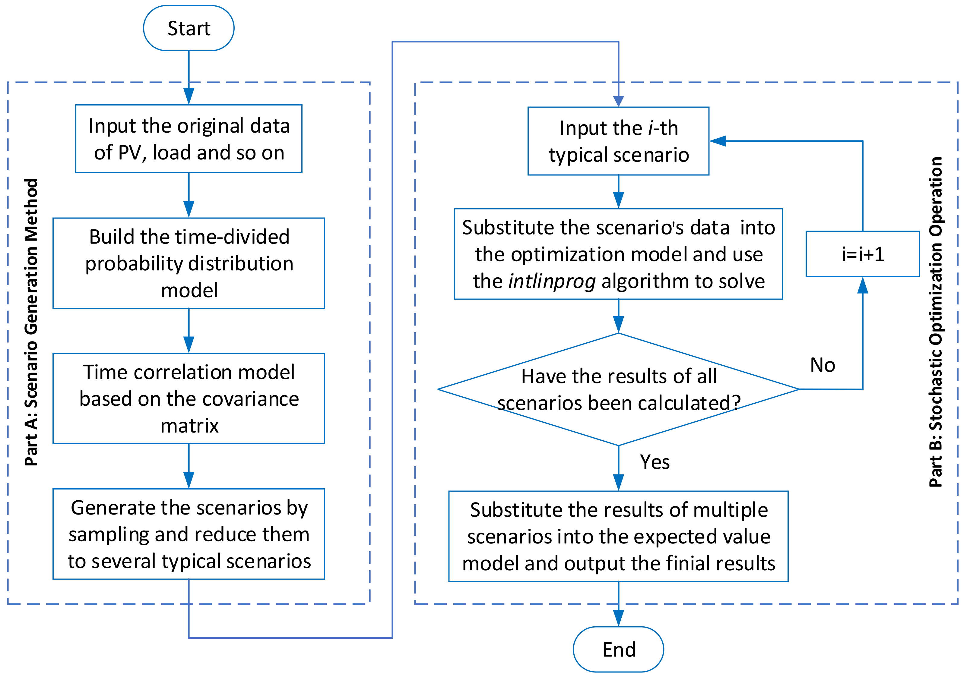
2. Scenario Generation Method

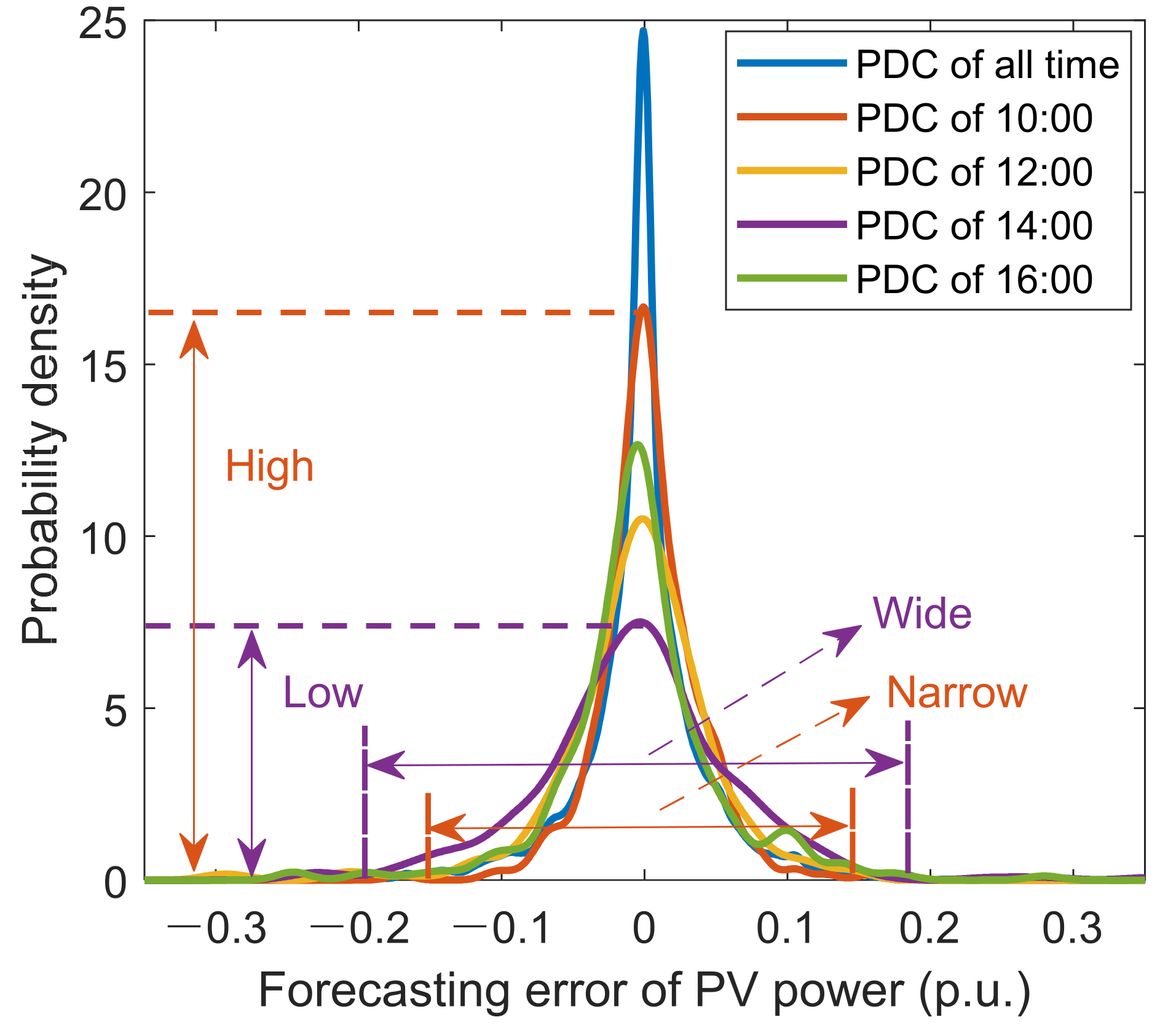
2.1. Time-Divided Probability Distribution Model of Forecasting Error

The probability density function can completely describe the statistical law of random variables, such as PV or load. Therefore, the probability distribution model is the basis of scenario generation. Existing studies usually assume that probability distribution models for different times are the same [20,21]. For example, the sampling time is 1 h, and scenario generation randomly generates errors for 24 h a day by using the same probability distribution model. However, in practice, the probability density function of the forecasting error at each moment is different. Generating scenarios with this method will obviously increase the error of power scenarios. Inspired by the distribution law of actual data, this paper proposes that the different probability distribution models should be created for different periods.

Moreover, the forecasting errors of various uncertain factors are assumed to be the normal distribution in references [20,21,28]. The distribution of random variables is usually unknown. The assumption that the forecasting errors are the normal distribution or t-distribution will also result in sampling errors. Kernel density estimation, a kind of nonparametric estimation model that is not based on the basic assumption of the distribution type, is a method to study the distribution characteristics of the data completely from the data samples. Reference [29] uses the nonparametric kernel density estimation to build the probability distribution model of wind power predicted errors, but still does not consider the characteristics of different periods. Therefore, to avoid sampling errors, this paper proposes using nonparametric kernel density estimation to build a probability distribution model of different periods.

Assuming that $x_1,x_2,\dots ,x_n$ is $n$ sample points (e.g., PV power) of independent identical distribution $F$, its probability density function is set as $f$, and the kernel density is estimated as follows:

$$\widehat{f}(x)=\frac{1}{nh}{\displaystyle \sum _{i=1}^{n}K\left(\frac{x-x_i}{h}\right)}$$

(1)

where $h$ is the bandwidth, $n$ is the sample number, and $K$ is the kernel function.

The kernel function $K\left(u\right)$ needs to satisfy the following conditions:

$$\left\{\begin{array}{c}{\displaystyle \int K(u)du}=1\\ {\displaystyle \int uK(u)du}=0\\ {\displaystyle \int u^{2}K(u)du}={\mu }_2(k)>0\end{array}\right.$$

(2)

The Gaussian kernel function is selected in this paper:

$$K\left(u\right)=\frac{1}{\sqrt{2\pi }}{e}^{-\frac{u^2}{2}}$$

(3)

In this section, the improvement on the model is that we build a probability density function for the forecasting error of each period, but not use the same model for all periods. In this paper, one day is divided into 24 periods, meaning that the sampling time is one hour. For each period, the kernel density estimation in Equation (1) is different.

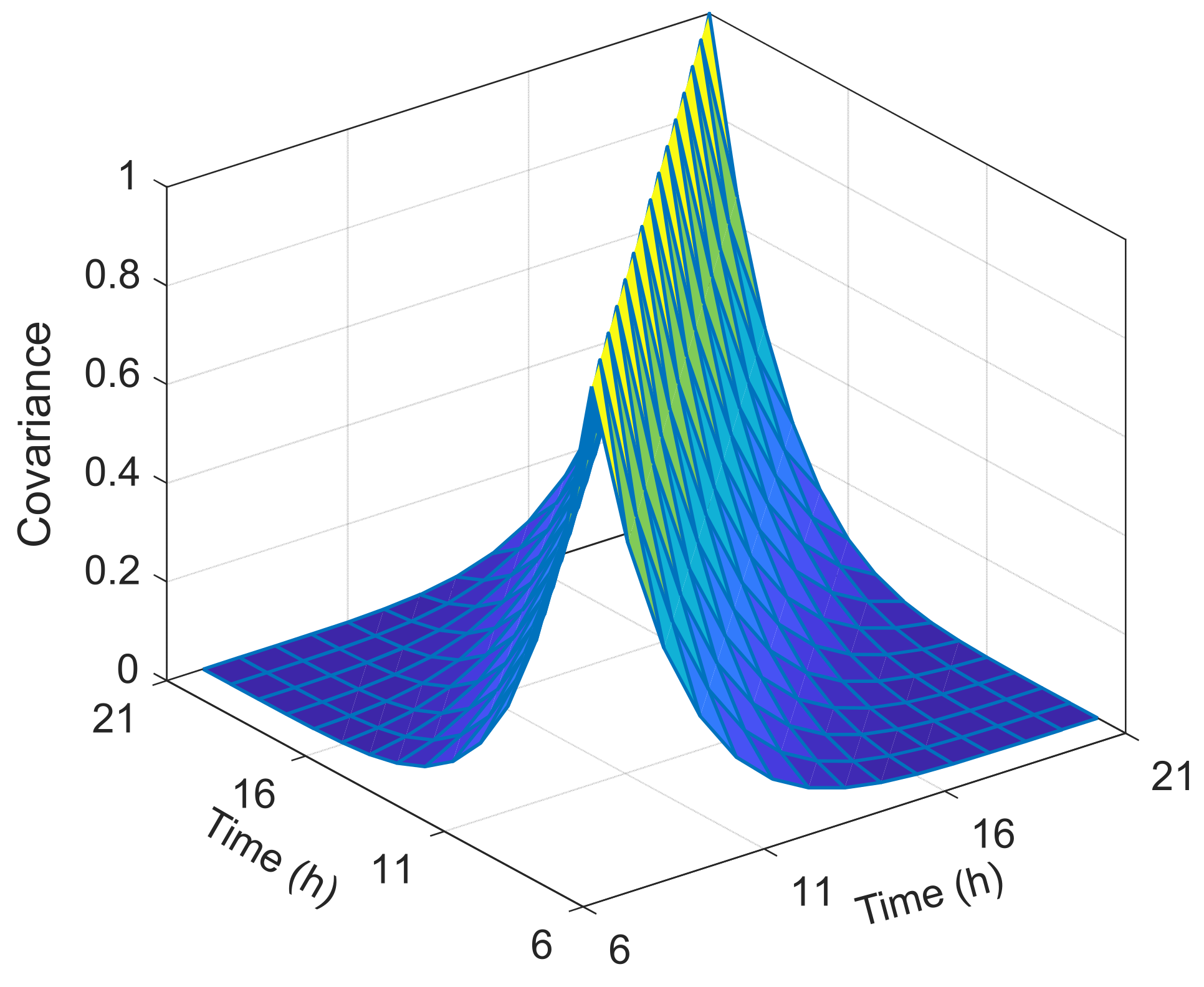
2.2. Multivariate Standard Normal Distribution

The scenario considering the time correlation refers to the power curve of the uncertain variables, such as PV or load. The time correlation needs to be considered when the scenario is generated by sampling the probability distribution models in Section 2.1. The probability distribution model is constructed by the nonparametric kernel density estimation method, and it is difficult to address the time correlation between them. Therefore, to construct the time correlation of different periods, the probability distribution model based on kernel density estimation needs to be transformed into a multivariate standard normal distribution [27]. To improve the sampling accuracy, the covariance parameters and the optimization method are improved in this section to improve the fitting accuracy of created scenarios to original scenarios.

The sampling process is converted into a sampling of multivariate standard normal distributions. The scenario can be viewed as a random vector $\mathit{Z}=(Z_1,Z_2,\dots ,Z_T)$, $T=24$. Since $\mathit{Z}$ follows the multivariate standard normal distribution, the covariance matrix can be expressed as [26]:

$$\sum =\left[\begin{array}{cccc}{\sigma }_{1,1}& {\sigma }_{1,2}& \cdots & {\sigma }_{1,T}\\ {\sigma }_{2,1}& {\sigma }_{2,2}& \cdots & {\sigma }_{2,T}\\ ⋮& ⋮& \ddots & ⋮\\ {\sigma }_{T,1}& {\sigma }_{T,2}& \cdots & {\sigma }_{T,T}\end{array}\right]$$

(4)

where ${\sigma }_{m_1,m_2}=\mathrm{cov}(Z_{m_1},Z_{m_2})$ is the covariance between $Z_{m_1}$ and $Z_{m_2}$, $m_1,m_2=1,2,\dots ,T$. $\sum$ is a positive definite matrix, and the value of all diagonal elements is one.

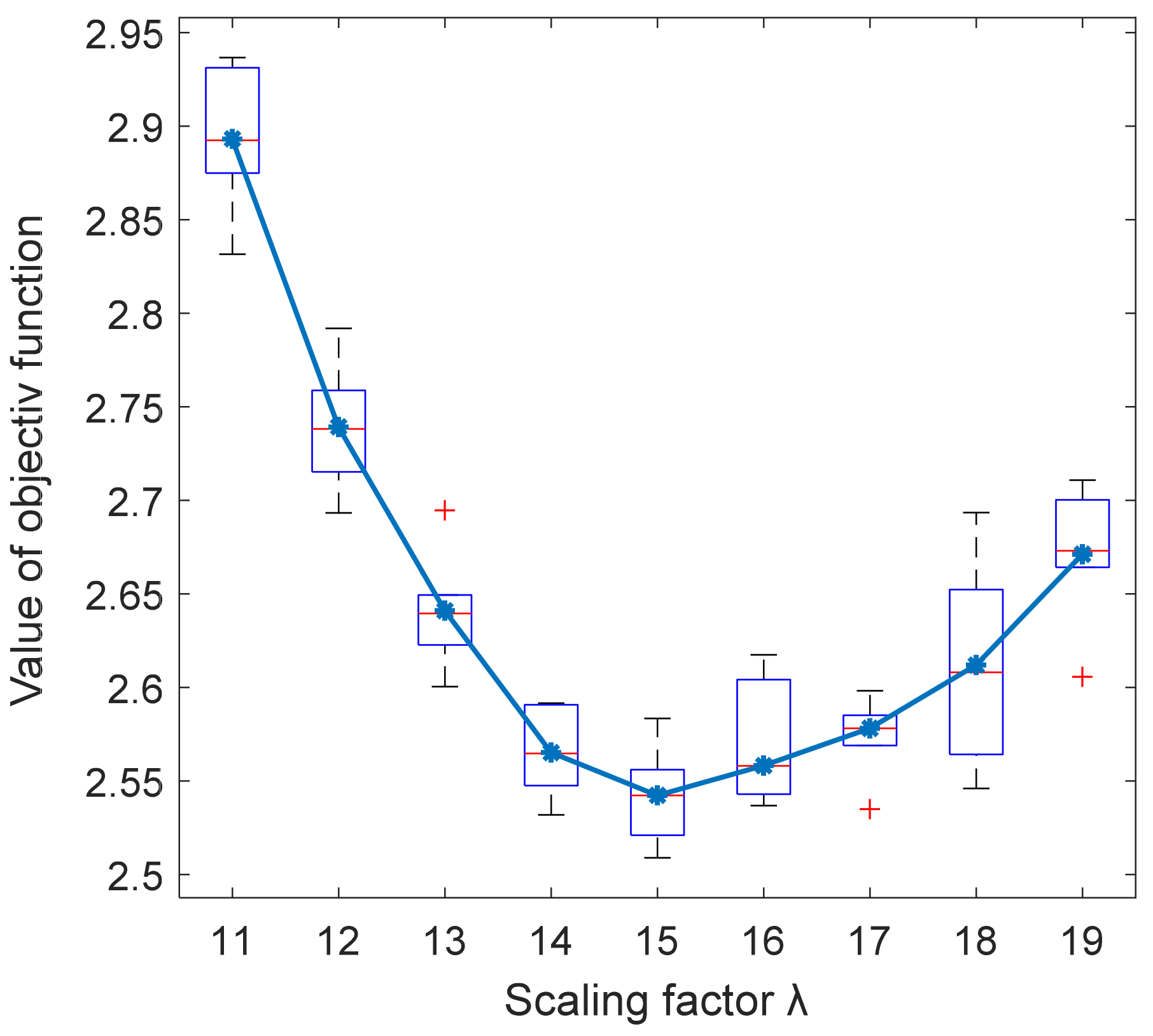
2.3. Covariance Parameter Optimization

In [27], the covariance expression is assumed to be the exponential form, but it isn’t compared with other expressions, such as power function. This paper proposes a novel covariance expression to test the adaptability. The covariance is assumed as follows:

$${\sigma }_{n,m}={\left(1-\frac{\left|m_1-m_2\right|}{\lambda }\right)}^{\alpha }$$

(5)

where $\lambda$ is the scaling factor and $\alpha$ is the exponent that is assumed to be a positive integer.

If the scaling factor and exponent are determined, the covariance matrix is uniquely determined. Therefore, the main goal is to find the best value of the scaling factor and exponent to ensure that the scenario generated by the multivariate standard normal distribution is as close as possible to the statistical features of the real data. The optimization objective function of the scaling factor and exponent is established as:

$$\min I={\displaystyle \sum _{i=1}^N\left|F(\Delta P_{t,i})-F^{\prime }(\Delta {P^{\prime }}_{t,i}^{})\right|}$$

(6)

where $N$ is the sampling number. $F(\Delta P_{}^{t,i})$ is the probability distribution function of real data. $\Delta P_{t,i}=P_{t,i}-P_{t-1,i}$ is the power fluctuation of real data. $F^{\prime }(\Delta P_{t,i}{}^{\prime })$ is the probability distribution function of the generated data. $\Delta P_{t,i}{}^{\prime }=P_{t,i}{}^{\prime }-P_{t-1,i}{}^{\prime }$ is the power fluctuation of generated data. When the objective function is minimum, the generated scenario is most consistent with the random characteristics of the original data, and the parameters $\lambda$ and $\alpha$ are optimal.

$$P_{R,t,s}=P_{R,t}^{forecast}+P_{R,t,s}^{error}$$

(7)

where $t=1,2,\dots ,T$, $s=1,2,\dots ,N$, $P_{R,t,s}$, $P_{R,t}^{forecast}$, and $P_{R,t,s}^{error}$ are the value of random variables, the forecasting value and the value of the forecasting error at time $t$, respectively. $R$ is the type of random variable, such as PV, electric load, and cooling load. $s$ is the scenario number.

A large number of scenarios can be generated by using the above method. If the scheduling calculation of the integrated energy microgrid is carried out based on a large number of scenarios, the calculation results will be more accurate, but the amount of calculation will be large and the calculation time will be very long. Therefore, a large number of scenarios need to be reduced to obtain a few representative scenarios and their probabilities. Since scenario reduction is not the main research content of this paper, it will not be repeated in this paper.

3. Stochastic Optimization Operation Model of an Integrated Energy Microgrid

In this section, the optimal operation model of the integrated energy microgrid is established. The integrated energy microgrid contains four energy forms: cooling energy, heating energy, electricity and gas. The IEMG contains a gas microturbine, PV power, wind power, battery, thermal storage tank, gas boiler, absorption chiller, electric chiller and various loads. A schematic diagram of the IEMG system is shown in Figure 1. Electric sources, including PV, wind power, gas microturbine and the power grid, supply power to the electrical load. In winter, the waste heating energy recovery device of the gas microturbine, gas boiler and heating system can provide the consumer with heating energy. The absorption chiller and electric chiller provide cooling energy for the user in summer. In addition, the battery and thermal storage tank can store and release electric and heating energy, respectively.

3.1. Optimization Model of Operation Cost

The objective function of the optimal operation of the integrated energy microgrid is to minimize the operating cost. The operating cost of the system includes the cost of purchasing electricity from the power grid $C_{grid}$ and the cost of purchasing gas $C_{fuel}$. The operating income is from selling electricity to the power grid $C_{sold}$. The optimization objective function is:

$$\min C=C_{grid}+C_{fuel}-C_{sold}$$

(8)

$$C_{grid}={\displaystyle \sum _{t=1}^T{c}_{grid,t}{P}_{grid,t}\Delta t}$$

(9)

$$C_{fuel}={\displaystyle \sum _{t=1}^T\left[c_{ng,t}\left(G_{gt,t}+G_{gb,t}\right)/H{V}_{ng}\right]\Delta t}$$

(10)

$$C_{sold}={\displaystyle \sum _{t=1}^T{c}_{sold,t}{P}_{sold,t}\Delta t}$$

(11)

where $c_{grid,t}$ is the electricity price, $P_{grid,t}$ is the power purchased from the grid, $\Delta t$ is the time interval, $c_{ng,t}$ is the natural gas price, $G_{gt,t}$ and $G_{gb,t}$ are the heating energy of the gas microturbine and gas boiler, respectively. $H{V}_{ng}$ is the natural gas heating value, $c_{sold,t}$ is the price of selling electricity to the grid, and $P_{sold,t}$ is the power sold to the power grid.

The optimal operation model should follow many constraints. The specific constraints are as follows.

(1) Cooling power balance constraint

The cooling power released by the absorption chiller and electric chiller should be equal to the cooling power load of the user.

$$CO{P}_{ac}{H}_{ac,t}+CO{P}_{ec}{P}_{ec,t}=C{P}_{L,t}$$

(12)

where $CO{P}_{ac}$ is the coefficient of performance of the absorption chiller, $H_{ac,t}$ is the heating power input into the absorption chiller, $CO{P}_{ec}$ is the coefficient of performance of the electric chiller, $P_{ec,t}$ is the electric power input into the electric chiller, and $C{P}_L$ is the cooling power of load.

(2) Heating power balance constraint

$$H_{hr,t}+H_{gb,t}-H_{ac,t}-H_{tst,dis,t}+H_{tst,ch,t}=H_{L,t}/{\eta }_{he}$$

(13)

where $H_{hr,t}$ is the heating power absorbed by the waste heat recovery device, $H_{gb,t}$ is the heating power generated by the gas boiler, $H_{ac,t}$ is the heating power input to the absorption chiller, $H_{tst,dis,t}$ and $H_{tst,ch,t}$ are the charging and discharging heating power of the thermal storage tank, respectively, $H_{L,t}$ is the heating load, and ${\eta }_{he}$ is the efficiency of the heating exchanger. The efficiency is a simplified value without considering the different application scenarios or types of equipment.

(3) Electric power balance constraint

$$P_{mt,t}+P_{grid,t}-P_{ec,t}+P_{b,dis,t}-P_{b,ch,t}-P_{sold,t}=P_{L,t}-P_{PV,t}-P_{W,t}$$

(14)

where $P_{mt,t}$ is the gas microturbine output power, $P_{grid,t}$ is the power purchased from the grid, $P_{ec,t}$ is the input electric power of the electric chiller, $P_{b,ch,t}$ and $P_{b,dis,t}$ are the charging and discharging power of the battery, $P_{sold,t}$ is the power sold to the grid, $P_{L,t}$ is the electric load, $P_{PV,t}$ is the PV power, and $P_{W,t}$ is the wind power.

(4) The constraint of the gas microturbine

This paper assumes that the electric power of the micro gas turbine has a relationship with its heating value and the efficiency is a fixed value.

$$P_{mt,t}=G_{gt,t}{\eta }_{mt}$$

(15)

$$P_{mt}^{\min }\le P_{mt,t}\le P_{mt}^{\max }$$

(16)

where ${\eta }_{mt}$ is the efficiency of the gas microturbine and $P_{mt}^{\min }$ and $P_{mt}^{\max }$ are the minimum and maximum values of the gas microturbine power, respectively.

(5) The constraint of the battery

$$S\mathrm{o}{C}_{b,t}=S\mathrm{o}{C}_{b,t-1}\left(1-{\sigma }_b\right)+{\eta }_{b,ch}{P}_{b,ch,t}\mathrm{\Delta }t/E_{b\_N}\text{-}{\eta }_{b,dis}{P}_{b,dis,t}\Delta \mathrm{t}/E_{b\_N}$$

(17)

$$\left\{\begin{array}{c}0\le P_{b,ch,t}\le u_b{P}_b^{\max }\\ 0\le P_{b,ch,t}\le \left(1-u_b\right)P_b^{\max }\end{array}\right.$$

(18)

$$S\mathrm{o}{C}_b^{\min }\le S\mathrm{o}{C}_t\le S\mathrm{o}{C}_b^{\max }$$

(19)

$$u_b=0 \mathrm{or} 1$$

(20)

$$S\mathrm{o}{C}_{b,1}^{}=S\mathrm{o}{C}_{b,24}^{}$$

(21)

where $S\mathrm{o}{C}_{b,t}$ is the state of charge of the battery, ${\eta }_{b,ch}$ and ${\eta }_{b,dis}$ are the charging and discharging efficiency, respectively. $P_{b,ch,t}$ and $P_{b,dis,t}$ are the charging and discharging power, $E_{b\_N}$ is the rated energy of the battery, $P_b^{\max }$ is the maximum power, and $S\mathrm{o}{C}_b^{\min }$ and $S\mathrm{o}{C}_b^{\max }$ are the minimum and maximum state of charge (SoC), respectively. $u_b$ is the 0–1 variable related to the battery.

In this paper, we take one day or 24 h as a cycle period, in which we assume that the initial and end states of the energy storage battery are the same. This assumption is also suitable for the thermal storage tank.

(6) The constraint of interactive electric power with a power grid

$$\left\{\begin{array}{c}0\le P_{grid,t}\le u_g{P}_{grid}^{\max }\\ 0\le P_{sold,t}\le \left(1-u_g\right)P_{grid}^{\max }\end{array}\right.$$

(22)

$$u_g=0 \mathrm{or} 1$$

(23)

where $P_{grid}^{\max }$ is the maximum interactive power and $u_g$ is the 0–1 variable related to the interactive electric power.

(7) The constraint of the thermal storage tank

$$E_{tst,t}=E_{tst,t-1}\left(1-{\sigma }_{tst}\right)+{\eta }_{tst,ch}{H}_{tst,ch,t}\Delta \mathrm{t}\text{-}{H}_{tst,dis,t}\Delta \mathrm{t}/{\eta }_{tst,dis}$$

(24)

$$\left\{\begin{array}{c}0\le H_{tst,ch,t}\le u_{tst}{H}_{tst}^{\max }\\ 0\le H_{tst,disch,t}\le \left(1-u_{tst}\right)H_{tst}^{\max }\end{array}\right.$$

(25)

$$u_{tst}=0 \mathrm{or} 1$$

(26)

$$E_{tst}^{\min }\le E_{tst,t}\le E_{tst}^{\max }$$

(27)

$$E_{tst,1}=E_{tst,24}$$

(28)

where $E_{tst,t}$ is the heating energy stored in the thermal storage tank. ${\eta }_{tst,ch}$ and ${\eta }_{tst,dis}$ are the charging and discharging efficiencies of the thermal storage tank, respectively. $H_{tst,ch,t}$ and $H_{tst,dis,t}$ are the charging and discharging heating power, respectively, and $H_{tst}^{\max }$ is the maximum heating power. $E_{tst}^{\min }$ and $E_{tst}^{\max }$ are the minimum and maximum heating energies, respectively, and $u_{tst}$ is the 0–1 variable related to the thermal storage tank.

3.2. Expected Model of Operating Cost

The forecasting error scenarios of user load, PV, etc., can be generated by the method in Section 2. The typical scenarios and their corresponding probabilities are assumed to be:

$$\left(S_i,{\xi }_i\right), i=1,2,\dots ,n.$$

(29)

$$S_i\sim \left(P_{PV},P_W,P_L,C{P}_L,H_L\right)$$

(30)

where $P_{PV},P_W,P_L,C_L,H_L$ are the PV power, wind power, electric load, cooling load and heating load.

Based on the multi-scenario method, the stochastic optimization problem is transformed into several deterministic problems, and the input of each deterministic problem is one typical scenario. The user cost model can be solved in each scenario. Then, the expected value of the user operating cost can be obtained by the expected value model:

$$E\left(C\right)={\displaystyle \sum _{n=1}^N{\xi }_n{C}_n}$$

(31)

where ${\xi }_n$ and $C_n$ are the probability and the cost corresponding to scenario $n$, respectively.

3.3. Solving Method and Steps

In the model of Section 3.1, the relationship of decision variables is linear, except for Equations (20), (23) and (26). The decision variables in these three equations are all integers. Therefore, this paper uses the intlinprog algorithm in MATLAB to solve the stochastic optimization model. The intlinprog algorithm is a mixed-integer linear programming method. The flow chart of this paper is shown in Figure 2.

The flow chart is divided into two parts. Part A is the scenario generation method and Part B is the stochastic optimization operation. The specific solution steps are as follows:

Part A: Scenario generation method.

Step 1: Input the original data of PV, load and so on.

Step 2: Build the time-divided probability distribution model.

Step 3: Build the time correlation model based on the covariance matrix of multivariate standard normal distribution.

Step 4: Generate the scenarios by sampling the probability distribution model with the time correlation and reduce them to several typical scenarios.

Part B: Stochastic optimization operation.

Step 1: Input the i-th scenario, $i=1,2,\dots ,n.$.

Step 2: Substitute the scenario’s data into the optimization model in Section 3.1 and solve the model using the intlinprog algorithm in MATLAB.

Step 3: Determine that the calculations of all the typical scenarios are complete. If so, execute the next step. If not, $i=i+1$ and return to the first Step 1, Part B.

Step 4: Substitute the optimization results of all scenarios into Equation (31) to solve the expected value of the operating cost and output the calculation results.

As seen in the above steps, each typical scenario is taken as input to solve the optimization problem. Therefore, the solving process of the optimization problem is executed $n$ times, which is also the number of typical scenarios.

4. The Results and Analysis

To verify the method proposed in this paper, a microgrid system was adopted for simulation calculation. It is located in an industrial park in Changzhou, Jiangsu Province, China. Based on this system, we built an integrated energy microgrid.

Table 1. Equipment Parameters in the Integrated Energy Microgrid.

Equipment	Parameters
Gas microturbine	$P_{mt}^{\min }=0 \mathrm{kW}$$, P_{mt}^{\max }=120 \mathrm{kW}$$, {\eta }_{mt}=0.3$
Gas boiler	$H_{gb\_N}^{}=300 \mathrm{kW}$
PV power	$P_{PV\_N}^{}=150 \mathrm{kW}$
Absorption chiller	$CO{P}_{ac}=0.7$$, H_{ac}^{\max }=500 \mathrm{kW}$
Electric chiller	$CO{P}_{ec}=4$$, P_{ec}^{\max }=100 \mathrm{kW}$
Wind power	$P_{W\_N}^{}=150 \mathrm{kW}$
Battery	${\eta }_{b,ch}={\eta }_{b,dis}=0.95$$, P_b^{\max }=100 \mathrm{kW}$$, E_{b\_N}=200 \mathrm{kW}$, $S\mathrm{o}{C}_b^{\min }=10\%$$S\mathrm{o}{C}_b^{\max }=90\%$
Thermal storage tank	${\eta }_{tst,ch}={\eta }_{tst,dis}=0.9$, $H_{tst}^{\max }=300 \mathrm{kWh}$$, E_{tst}^{\min }=0 \mathrm{kWh}$, $E_{tst}^{\max }=300 \mathrm{kWh}$
Exchange power with grid	$P_{grid}^{\max }=300 \mathrm{kW}$
Heating exchanger	${\eta }_{he}=0.75$

shows the corresponding parameters of various equipment in the integrated energy microgrid.

4.1. Probability Distribution Model

Figure 3 shows the histogram and distribution curves of the forecasting error of PV power. The histogram of the forecasting error of PV power is shown in the blue bar and is related to the left vertical axis, the frequency. The fitting probability density distribution function curve is shown in red curve and is related to the right vertical axis, the probability density. The horizontal axis is the per-unit value of the forecasting error. As mentioned above, we need to establish the probability distribution model of PV forecasting error in each period. We take 8:00 and 14:00 as examples to explain the results, which are shown in Figure 3a,b, respectively. In Figure 3a, compared with the histogram, the fitting effect of the normal distribution is the worst, and the fitting effects of the kernel density distribution and the t-distribution are similar. The main difference between these two distributions is in the range of ±[0.02, 0.05]. The shape of the kernel density distribution curve has more fluctuations to fitting the shape of the histogram, while the t-distribution does not have this advantage. The root mean square error (RMSE) of the two distributions are $4.44\times {10}^{-4}$ and $9.45\times {10}^{-4}$, respectively. The fitting effect kernel density distribution is better. At 14:00, the fitting effect of the kernel density distribution and t-distribution is almost the same.

To compare the forecasting error probability distribution of different periods, we calculated the RMSE of the different distributions, as shown in Figure 4. The vertical axis is the RMSE value between the cumulative probability distribution curve and the fitting probability distribution curve. The fitting effect of the normal distribution is the worst, and the effects of the t-distribution and nonparametric kernel density distribution (NKDD) at 10:00–20:00 are very similar. In the morning and evening, the effect of the nonparametric kernel density distribution is better than the t-distribution. Therefore, the nonparametric kernel density distribution model adopted in this paper is feasible and has advantages. For all periods, the total RMSE of NKDD is 49.00% and 90.37% lower than the t-distribution and the normal distribution, respectively.

Figure 5 is the probability density curve (PDC) of selected periods. The horizontal axis is the forecasting error of PV power, and the vertical axis is the probability density. The curve marked by “PDC of all time” refers to the probability distribution curve of errors of all periods. The other curves are the probability density curve of each period. We can see that the distributions of different periods are different. Taking the 10:00 and 14:00, for example, the shape of the probability density curve at 10:00 is higher and narrower than the shape of the probability density curve at 14:00. The curve of all time is highest and narrowest. The reason is that the PV power in the morning and at nightfall is low and closed to zero. Owing to the irregular shape of the probability density curve, a nonparametric kernel density distribution has more advantages. Therefore, if the scenario is generated by sampling based on the distribution function of all errors, the errors of the generated scenario will be too large. Based on the time-divided probability distribution for sampling, the statistical law of the generated scenario is more consistent with the original data.

4.2. The Analysis of the Time Correlation

In general, the time correlation exists between probability distribution models of different times. In Section 2, the covariance matrix was used to calculate the time correlation, and its parameters were optimized. Based on this method, the time correlation between probability distribution models is simulated and analyzed in this section. We carried out a sensitivity analysis of the exponent $\alpha$ and scaling factor $\lambda$.

Figure 6 shows the objective function value comparison of the different exponents $\alpha$ and scaling factors $\lambda$. In Equation (6), we defined the optimization objective function of the scaling factor and exponent, which represents the relationship between the time correlation and covariance. The smaller it is, the higher the sampling accuracy. Figure 6 shows the value of the objective function of different $\alpha$ values and the scaling factor $\lambda$. As the value of the two parameters increases, the objective value decreases first and then increases. When the exponent $\alpha$ and the scaling factor $\lambda$ are 6 and 15 respectively, the objective value is smallest, and the consistency of statistical characteristics between the generated scenario and the original data is highest.

Figure 7 shows a boxplot of the relationship between the objective function value and scaling factor $\lambda$. The boxplot can show the maximum, minimum and average values of multiple calculations to avoid the randomness of the calculation results. As shown in Figure 7, within a certain range [11,19], the scaling factor decreases first and then increases, and the average objective value reaches the minimum of 2.5423 when the scaling factor $\lambda$ is 15. As mentioned above, when the objective function value is minimal, the time correlation of the generated scenarios is closest to the real data. For the scenario without considering the time correlation, the objective function value is 9.728. The optimal value of this paper’s method is 73.87% lower than 9.728. For the method in [27], the optimal objective function value is 2.6745 when the range parameter is 3. The optimal value of this paper’s method is 5.66% lower than 2.6745.

When the objective function value is minimum, the relationship between the covariance and time is shown in Figure 8. Obviously, the correlation between the same time is 1. The covariance decreases rapidly with the increase of the time difference, such as the covariances between 7 and 8, 9, 10, 11, 12 o’clock are 0.66, 0.26, 0.16, 0.09, 0.05, respectively. This covariance decrease is also in line with the objective law and subjective cognition. For the other values of the scaling factor and exponent, the variation trend of covariance is different, which has an impact on the time correlation of the forecasting error of PV power and lead to inconsistency between the statistical law of the generated scenarios and the actual scenarios.

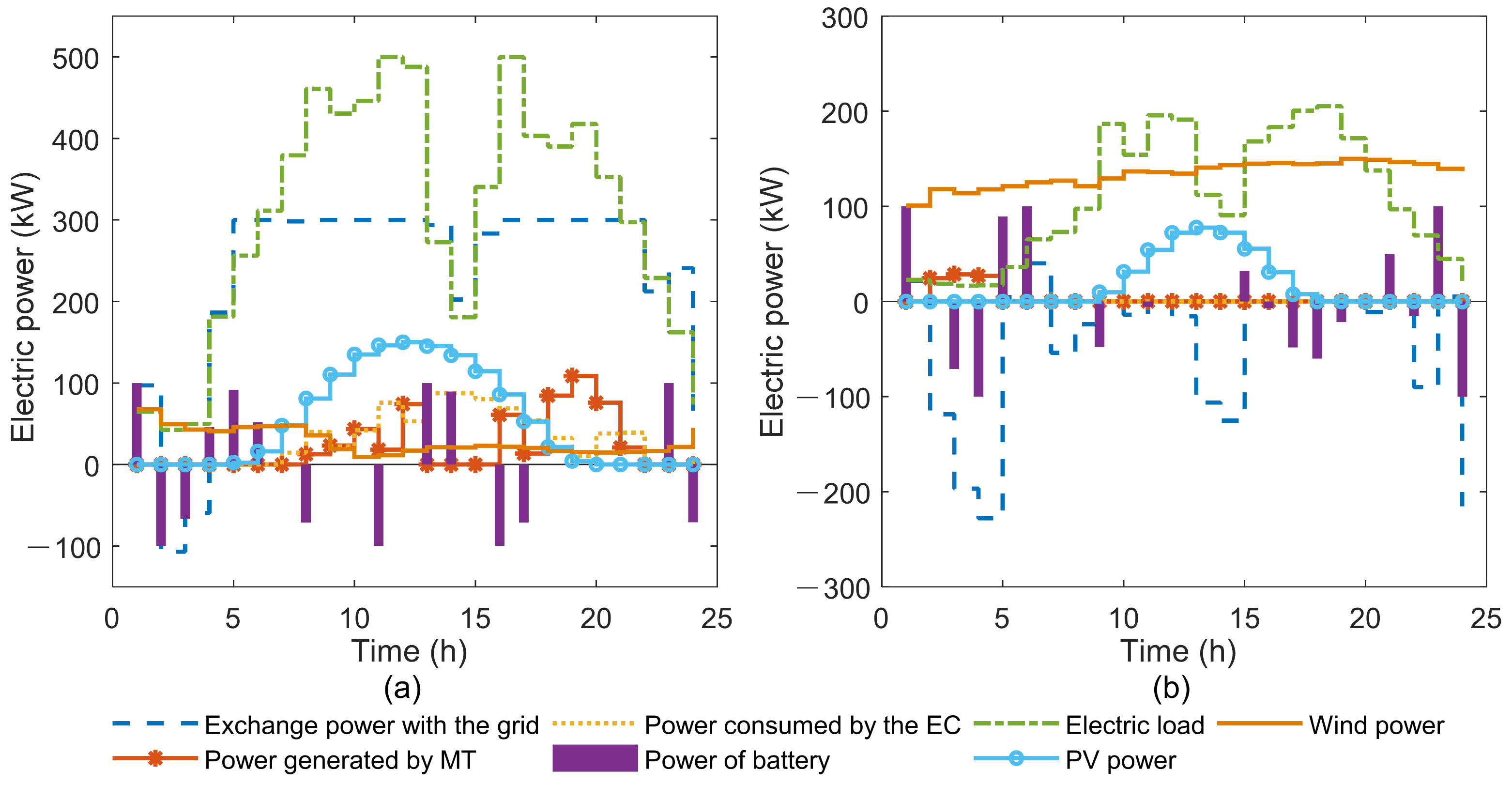
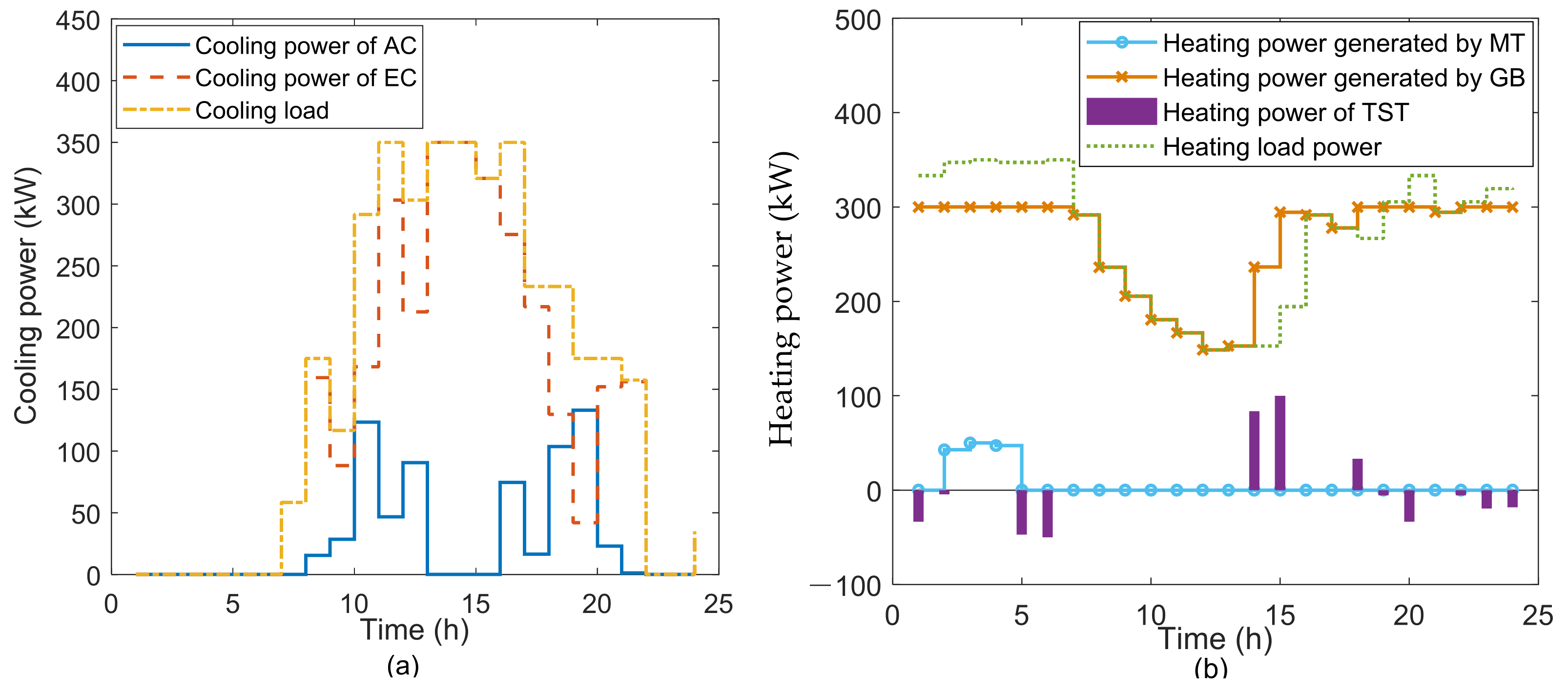
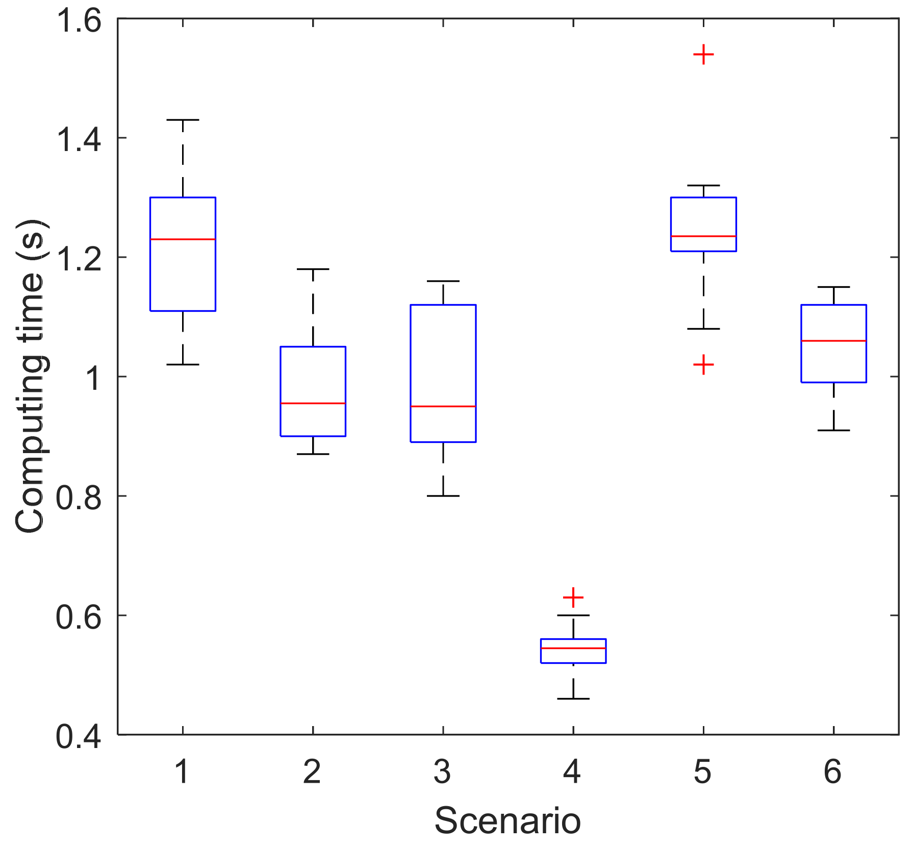
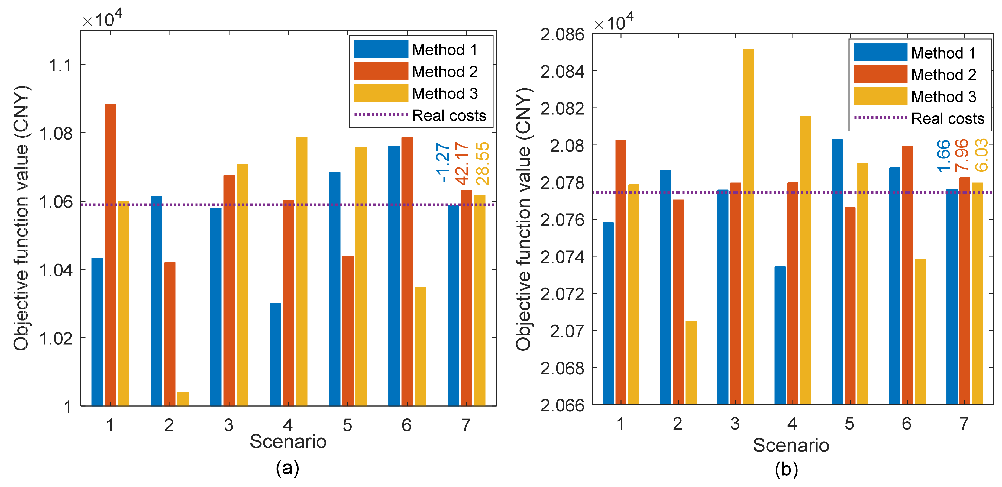
4.3. Optimized Operation of Integrated Energy Microgrid

According to the optimized operation model proposed in Section 3, the simulation analysis is carried out in this section. In Figure 9 and Figure 10, the input data of the simulation are the point forecasting scenario. We assume that the typical day in summer has a cooling load and does not have a heating load, and the typical day in winter has a heating load and does not have a cooling load.

As seen from Figure 9a, the balance of electric power can be achieved among the power supply, load and battery. The battery energy storage system has two functions. One function is to charge when the electricity price is low and then release electric energy to earn profits. The other function is to meet the electrical demand during peak load periods. Between 1:00 and 6:00, the battery earns profits by charging when the electricity price is low and discharging when the electricity price is high. The electricity demand is large at 8:00 and 11:00. Although the electricity price is high at 12:00 and 13:00, to avoid the load demand not being met at 16:00 and 17:00, the battery must charge during the period of high electricity price. Energy storage plays an important role in meeting the demand of electric load and making profits for the user.

In summer, the micro gas turbine can provide electrical power for electric load and provide heating energy for the absorption chiller at the same time. As shown in Figure 9a and Figure 10a, the user has the cooling power demand from 7:00 to 22:00, which is supplied mainly by the electrical chiller. Besides, the user’s electricity load power is high, and a gas microturbine supplies power to the user. At the same time, the gas microturbine generates heating energy, which can be used by the absorption chiller to generate cooling power at 8:00–13:00 and 16:00–21:00.

As shown in Figure 9b, the case we selected in winter has higher wind power and lower load power, and the integrated energy microgrid can sell electricity to the grid to make profits most of the time. Since wind-PV power generation can meet most of the load demand, the main role of energy storage batteries is to make profits by charging when the price is low and discharging when the price is high. As seen from Figure 9b and Figure 10b, the heating load of users is met mainly by the gas-fired boiler. When the gas-fired boiler reaches its output limit, such as at 1:00 and 7:00, part of the heating load is met by the thermal storage tank, and the other part is met by the micro gas turbine. The main function of the thermal storage tank is to store heating energy when the heating load is low and release heating energy when the heating demand is high. The thermal storage tank stores the heating energy generated by the gas-fired boiler from 14:00 to 15:00. The thermal storage tank releases heating energy when the gas-fired boiler cannot meet the heating demand from 19:00 to 23:00.

The simulation results of Figure 9 and Figure 10 are based on the input of point forecasting data. However, the forecasting of PV, wind power and load has errors in real applications. In particular, the electric energy storage battery and thermal storage tank both have a time-coupling relationship. Their action at one moment will have an impact on their operation in the future. Therefore, we proposed the stochastic optimization operation model based on the multiple scenarios in Section 3.1 and Section 3.2.

Based on the model in Section 2 and the corresponding simulation results and taking PV power as an example, we generated 10,000 random scenarios and reduced them to six typical scenarios. As mentioned in Section 3.3, the executed times of solving the optimization problem are equal to the whole time of typical scenarios. Thus, the optimization problem is solved six times in this case. The intlinprog algorithm can display the computing time. We repeated the calculation ten times for each scenario and plotted the boxplot of the computing time of six different scenarios in Figure 11, which has different numbers of iterations and computing times. One of the reasons why the computing time is different is that the feasible domains for the optimization models in the different scenarios are different. As seen from the boxplot, the computing time for the six typical scenarios is in the range of [0.4,1.6], which is not very long in total. However, if the computation is performed for 10,000 scenarios, the solution time would be very long. It is worth noting that the computing time of the fourth scenario is shortest. The branch and bound algorithm of intlinprog algorithm is used in this paper. Its computing time is different if the feasible domains and initial value of the variables. For the fourth scenario, its calculation requires the least branch and bound steps, so the computing time is shortest.

In this paper, the time correlation of the time-divided probability distribution models is considered when generating scenarios but has not been considered in the literature [17]. In addition, the time correlation considered in [27] is not very consistent with the statistical laws of real data. To analyze and consider whether the time correlation would have an impact on the operating results, we took PV power generation as a single variable and carried out a simulation. We compared the operating costs under three different sets of typical scenarios generated by three methods. The results are shown in Figure 12. The blue histogram or Method 1 is the costs of the scenarios set that considers the time correlation using the method in this paper. The red histogram or Method 2 is the costs of the scenario set that does not consider the time correlation. The yellow histogram or Method 3 is the cost of the scenario set that considers the time correlation in [27]. The real costs are the costs of a real scenario but not the forecasting scenario. The vertical axis represents the value of the objective function in the Chinese yuan (CNY). On the horizontal axis, 1–6 represents six typical scenarios, and 7 represents the results of the expected value model of the six scenarios.

As shown in Figure 12a, in summer, the operating costs in different scenarios are different. We are more concerned about the expected value of three scenario sets, that is, scenario 7. Compared with the real value, the costs of the method in this paper are 1.27 less than the actual value, while the costs of the methods in [17,27] are 42.17 and 28.55 more than the actual value, respectively. The difference is reduced by 96.98% and 95.55%, proving that the expected costs of the method proposed in this paper are closer to the actual value.

For Figure 12b, in winter, there is a similar conclusion. The differences between the three methods are 1.66, 7.96 and 6.03. The difference in this paper is reduced by 79.17% and 72.47% because the PV power in winter is smaller than the PV power in summer. In Figure 12a,b, the costs of our method are higher and lower than the real scenario, respectively. This phenomenon that the cost fluctuates higher or lower than the real scenario is very normal, owing to the stochastic influence of the weather for the PV power generation. What we focus on is that the influence caused by the stochastic weather or the absolute value of cost is decreased. In two seasons, the comparison of the three scenario sets shows that the scenario generation method proposed in this paper considers the correlation of different periods and has less impact on the operation results.

5. Conclusions

This paper proposes an advanced scenario generation method and applies it to the stochastic optimization operation of integrated energy microgrid, which includes electric, cooling, heating power, and natural gas. In this method, the time correlation of the time-divided probability distribution models is considered in the process of generating scenarios. Based on multiple scenario theory, the stochastic optimization operation model was built. The main conclusions are as follows.

(1) This paper established a time-divide probability distribution model based on nonparametric kernel density estimation. The simulation results show that the fitting effect of the NKDD estimation model is better than the fitting effect of the normal distribution and t-distribution.

(2) Considering the time correlation of the time-divided probability distribution models, this paper proposes the covariance expression and the optimization model of its parameters. Compared with other methods with and without considering the time correlation, the statistical characteristics of scenarios generated by this paper’s method are more consistent with the real data.

(3) A stochastic optimization operation model based on the expected value model is established for the integrated energy microgrid. The model can achieve the energy balance in the system, and the operating cost difference is reduced, which proves the feasibility and economy of the operation model.

Although we obtained some research results, we still need to explore more methods that consider more factors related to uncertainty, such as other forms of covariance matrices and the uncertainty of price. In addition, our optimization model needs to take more economic factors into account. Many factors, such as the efficiency of the gas microturbine and the heating exchanger, are simplified and assumed as a fixed value. In future work, we will refine our optimization model based on the accurate forecasting of uncertain factors. The models with more refined and specific parameters will be built too. Moreover, the planning method of the integrated energy system is a research hotspot. We will study the planning of the IES microgrid considering the uncertainty and apply stochastic optimization methods in a large-scale integrated energy system.

References

1. Chen, Y.; Deng, C.; Yao, W.; Liang, N.; Xia, P.; Cao, P.; Dong, Y.; Zhang, Y.-A.; Liu, Z.; Li, D.; et al. Impacts of stochastic forecast errors of renewable energy generation and load demands on microgrid operation. Renew. Energy 2019, 133, 442–461. [Google Scholar] [CrossRef]
2. Zakernezhad, H.; Nazar, M.S.; Shafie-Khah, M.; Catalão, J.P. Optimal resilient operation of multi-carrier energy systems in electricity markets considering distributed energy resource aggregators. Appl. Energy 2021, 299, 117271. [Google Scholar] [CrossRef]
3. Yang, Z.; Wu, R.; Yang, J.; Long, K.; You, P. Economical Operation of Microgrid with Various Devices Via Distributed Optimization. IEEE Trans. Smart Grid 2015, 7, 857–867. [Google Scholar] [CrossRef]
4. Gan, W.; Yan, M.; Yao, W.; Guo, J.; Ai, X.; Fang, J.; Wen, J. Decentralized computation method for robust operation of multi-area joint regional-district integrated energy systems with uncertain wind power. Appl. Energy 2021, 298, 117280. [Google Scholar] [CrossRef]
5. Marino, C.; Marufuzzaman, M.; Hu, M.; Sarder, M. Developing a CCHP-microgrid operation decision model under uncertainty. Comput. Ind. Eng. 2018, 115, 354–367. [Google Scholar] [CrossRef]
6. Wang, Q.; Liu, J.; Hu, Y.; Zhang, X. Optimal Operation Strategy of Multi-Energy Complementary Distributed CCHP System and its Application on Commercial Building. IEEE Access 2019, 7, 127839–127849. [Google Scholar] [CrossRef]
7. Wang, Y.; Wang, Y.; Huang, Y.; Li, F.; Zeng, M.; Li, J.; Wang, X.; Zhang, F. Planning and operation method of the regional integrated energy system considering economy and environment. Energy 2019, 171, 731–750. [Google Scholar] [CrossRef]
8. Mu, C.; Ding, T.; Zeng, Z.; Liu, P.; He, Y.; Chen, T. Optimal operation model of integrated energy system for industrial plants considering cascade utilisation of heat energy. IET Renew. Power Gener. 2020, 14, 352–363. [Google Scholar] [CrossRef]
9. He, J.; Li, Y.; Li, H.; Tong, H.; Yuan, Z.; Yang, X.; Huang, W. Application of Game Theory in Integrated Energy System Systems: A Review. IEEE Access 2020, 8, 93380–93397. [Google Scholar] [CrossRef]
10. Yan, M.; He, Y.; Shahidehpour, M.; Ai, X.; Li, Z.; Wen, J. Coordinated Regional-District Operation of Integrated Energy Systems for Resilience Enhancement in Natural Disasters. IEEE Trans. Smart Grid 2019, 10, 4881–4892. [Google Scholar] [CrossRef]
11. Yi, Z.; Xu, Y.; Hu, J.; Chow, M.-Y.; Sun, H. Distributed, Neurodynamic-Based Approach for Economic Dispatch in an Integrated Energy System. IEEE Trans. Ind. Inform. 2019, 16, 2245–2257. [Google Scholar] [CrossRef]
12. Sun, Y.; Zhang, B.; Ge, L.; Sidorov, D.; Wang, J.; Xu, Z. Day-ahead optimization schedule for gas-electric integrated energy system based on second-order cone programming. CSEE J. Power Energy Syst. 2020, 6, 142–151. [Google Scholar] [CrossRef]
13. Guo, H.; Shi, T.; Wang, F.; Zhang, L.; Lin, Z. Adaptive clustering-based hierarchical layout optimisation for large-scale integrated energy systems. IET Renew. Power Gener. 2020, 14, 3336–3345. [Google Scholar] [CrossRef]
14. Yang, S.; Tan, Z.; Lin, H.; Li, P.; De, G.; Zhou, F.; Ju, L. A two-stage optimization model for Park Integrated Energy System operation and benefit allocation considering the effect of Time-Of-Use energy price. Energy 2020, 195, 117013. [Google Scholar] [CrossRef]
15. Chen, S.; Wang, S. An Optimization Method for an Integrated Energy System Scheduling Process Based on NSGA-II Improved by Tent Mapping Chaotic Algorithms. Processes 2020, 8, 426. [Google Scholar] [CrossRef] [Green Version]
16. Tan, Z.; Yang, S.; Lin, H.; De, G.; Ju, L.; Zhou, F. Multi-scenario operation optimization model for park integrated energy system based on multi-energy demand response. Sustain. Cities Soc. 2020, 53, 101973. [Google Scholar] [CrossRef]
17. Yan, R.; Lu, Z.; Wang, J.; Chen, H.; Wang, J.; Yang, Y.; Huang, D. Stochastic multi-scenario optimization for a hybrid combined cooling, heating and power system considering multi-criteria. Energy Convers. Manag. 2021, 233, 113911. [Google Scholar] [CrossRef]
18. Ma, X.-Y.; Sun, Y.-Z.; Fang, H.-L.; Tian, Y. Scenario-Based Multiobjective Decision-Making of Optimal Access Point for Wind Power Transmission Corridor in the Load Centers. IEEE Trans. Sustain. Energy 2012, 4, 229–239. [Google Scholar] [CrossRef]
19. Yoshida, K.; Negishi, S.; Takayama, S.; Ishigame, A. A stochastic scheduled operation of wind farm based on scenarios of the generated power with copula. Electr. Eng. Jpn. 2018, 205, 41–54. [Google Scholar] [CrossRef]
20. Mohammadi, S.; Soleymani, S.; Mozafari, B. Scenario-based stochastic operation management of MicroGrid including Wind, Photovoltaic, Micro-Turbine, Fuel Cell and Energy Storage Devices. Int. J. Electr. Power Energy Syst. 2014, 54, 525–535. [Google Scholar] [CrossRef]
21. Niknam, T.; Azizipanah-Abarghooee, R.; Narimani, M.R. An efficient scenario-based stochastic programming framework for multi-objective optimal micro-grid operation. Appl. Energy 2012, 99, 455–470. [Google Scholar] [CrossRef]
22. Zhao, L.; Huang, Y.; Dai, Q.; Yang, L.; Chen, F.; Wang, L.; Sun, K.; Huang, J.; Lin, Z. Multistage Active Distribution Network Planning With Restricted Operation Scenario Selection. IEEE Access 2019, 7, 121067–121080. [Google Scholar] [CrossRef]
23. Jafari, E.; Soleymani, S.; Mozafari, B.; Amraee, T. Scenario-based stochastic optimal operation of wind/PV/FC/CHP/boiler/tidal/energy storage system considering DR programs and uncertainties. Energy Sustain. Soc. 2018, 8, 2. [Google Scholar] [CrossRef] [Green Version]
24. Rachunok, B.; Staid, A.; Watson, J.-P.; Woodruff, D.L. Assessment of wind power scenario creation methods for stochastic power systems operations. Appl. Energy 2020, 268, 114986. [Google Scholar] [CrossRef]
25. Pinson, P.; Madsen, H.; Nielsen, H.A.; Papaefthymiou, G.; Klöckl, B. From probabilistic forecasts to statistical scenarios of short-term wind power production. Wind Energy 2009, 12, 51–62. [Google Scholar] [CrossRef] [Green Version]
26. Pinson, P.; Girard, R. Evaluating the quality of scenarios of short-term wind power generation. Appl. Energy 2012, 96, 12–20. [Google Scholar] [CrossRef] [Green Version]
27. Ma, X.-Y.; Sun, Y.-Z.; Fang, H.-L. Scenario Generation of Wind Power Based on Statistical Uncertainty and Variability. IEEE Trans. Sustain. Energy 2013, 4, 894–904. [Google Scholar] [CrossRef]
28. Bao, Z.; Qiu, W.; Wu, L.; Zhai, F.; Xu, W.; Li, B.; Li, Z. Optimal Multi-Timescale Demand Side Scheduling Considering Dynamic Scenarios of Electricity Demand. IEEE Trans. Smart Grid 2018, 10, 2428–2439. [Google Scholar] [CrossRef]
29. Zhou, B.; Ma, X.; Luo, Y.; Yang, D. Wind Power Prediction Based on LSTM Networks and Nonparametric Kernel Density Estimation. IEEE Access 2019, 7, 165279–165292. [Google Scholar] [CrossRef]
Figure 1. The diagram of integrated energy microgrid.
Processes 10 00330 g001
Figure 2. The flow chart of solving method.
Processes 10 00330 g002
Figure 3. The histogram and distribution function curve of PV forecasting error.
Processes 10 00330 g003
Figure 4. RMSE comparison of different distribution functions.
Processes 10 00330 g004
Figure 5. Probability density curves of different periods.
Processes 10 00330 g005
Figure 6. Correlation comparison of the different exponents and scaling factors.
Processes 10 00330 g006
Figure 7. The boxplot of the scaling factor λ .
Processes 10 00330 g007
Figure 8. Relationship between covariance and time difference.
Processes 10 00330 g008
Figure 9. Optimal operation results of electric power (a) summer (b) winter.
Processes 10 00330 g009
Figure 10. Optimal operation results of cooling power and heating power (a) The cooling power in summer cold (b) The heating power in winter.
Processes 10 00330 g010
Figure 11. Boxplot of the computing time for six different scenarios.
Processes 10 00330 g011
Figure 12. Comparison of Results in Different Scenarios (a) Summer (b) Winter.
Processes 10 00330 g012