Learning Dynamics Analysis: Assessing Generalization of Machine Learning Models for Optical Coherence Tomography Multiclass Classification

Abstract

This study evaluated the generalization and reliability of machine learning models for multiclass classification of retinal pathologies using a diverse set of images representing eight disease categories. Images were aggregated from two public datasets and divided into training, validation, and test sets, with an additional independent dataset used for external validation. Multiple modeling approaches were compared, including classical machine learning algorithms, convolutional neural networks with and without data augmentation, and a deep neural network using pre-trained feature extraction. Analysis of learning dynamics revealed that classical models and unaugmented convolutional neural networks exhibited overfitting and poor generalization, while models with data augmentation and the deep neural network showed healthy, parallel convergence of training and validation performance. Only the deep neural network demonstrated a consistent, monotonic decrease in accuracy, F1-score, and recall from training through external validation, indicating robust generalization. These results underscore the necessity of evaluating learning dynamics (not just summary metrics) to ensure model reliability and patient safety. Typically, model performance is expected to decrease gradually as data becomes less familiar. Therefore, models that do not exhibit these healthy learning dynamics, or that show unexpected improvements in performance on subsequent datasets, should not be considered for clinical application, as such patterns may indicate methodological flaws or data leakage rather than true generalization.

1. Introduction

Optical Coherence Tomography (OCT), first developed in the early 1990s, revolutionized medical imaging. This technique utilizes a continuous-wave light that is reflected from biological tissue, and the time-of-flight delays from different parts of the sample are collectively used to create an image [1]. This technology was further developed in the early 2000s to obtain in-vivo multi-layered scans of the human eye [2], giving way for enhancement of OCT imaging through the introduction of visible-light OCT [3]. While this technology has been applied in multiple medical fields, like cardiology [4] and gastroenterology [5], it cannot be denied that OCT scanning has gained most of its attention in the field of ophthalmology. OCT scans have allowed doctors to obtain vital information about the human eye and provide a different view of eye anatomy, greatly aiding in the diagnosis of different eye pathologies. For example, Spectral domain OCT (SD-OCT) has been shown as the leading diagnostic tool for neovascular age-related macular degeneration (AMD), allowing for detailed images of pigment epithelium fluid that builds up in the retinal layers during the progression of AMD [6]. Similarly, OCT scans have largely been adapted in the diagnosis of diabetic macular edema (DME). Diabetes has profound effects on the body’s vasculature, and that can largely be seen in the eyes. Leaking of fragile blood vessels can lead to retinal swelling and even permanent vision loss if left untreated. This swelling similarly puts patients at risk for retinal detachments, which largely require surgery. OCT scans have led the way for the rapid identification of diabetic retinal biomarkers, which have allowed for the detection of pathological tissue [7], as well as the response of the eye vasculature to DME treatment [8]. Likewise, OCT scans have become a vital tool in glaucoma detection and monitoring [9]. Undetected/untreated glaucoma can rapidly progress and even lead to complete vision loss. This makes for early detection and treatment a vital part of patient care. Similar to AMD detection, SD-OCT has shown the most potential in early glaucoma detection [10,11].

While the development of OCT scans has greatly enhanced the field of ophthalmology, there still remain aspects of the technology that pose challenges in diagnostics. For example, photos could have minimal imperfections or the OCT machines could have technical issues, collectively termed artifacts, which affect the image quality seen by the observer [12]. Since a large portion of OCT scans are manually analyzed by doctors, these artifacts could skew the analysis and lead to improper diagnosis and treatment planning for the patient [13,14]. Moreover, with the rising use of OCT scans, doctors are tasked with analyzing a multitude of scans at once, leading to the possibility of errors occurring due to misinterpretation. These concerns have collectively started to take center stage with the recent rise of machine learning (ML) and artificial intelligence (AI) in medicine and prominently within ophthalmology [15,16,17]. ML models have been developed to recognize and classify a wide range of retinal diseases. A Linear-support vector machine (SVM) model was found to have high specificity and sensitivity in the classification of DME [18]. Moreover, models have been developed to classify and track the progression of AMD, allowing for earlier intervention and properly guided treatment plans [19,20,21]. These applications of machine learning in ophthalmology have shown promising results, and new advancements are being made at an exponential rate.

However, it is important to note that while the application of ML has greatly progressed in the medical field, there are still quite a number of challenges that have to be faced and overcome before this technology can be further implemented in patient care. The number of publicly available datasets is often limited and those available have varying numbers of cases for each of the diseases, as well as disproportionate representation of different societal groups [22]. There is a lack of standardization for picture acquisition and processing, which could lead to the creation of artifacts. Moreover, due to inconsistent metrics during model performance analysis, it creates an environment in which no two models can be evenly compared to understand which would fit best into patient care [23,24]. ML and AI have also faced a great amount of scrutiny in a variety of professional fields, and even more so in the field of medicine with the risks to patient health that could result. Building upon this, the complexity of the ML systems does not help physicians understand the thought process behind how these systems determine diagnostic criteria [25].

While the challenges mentioned above will require the collaboration of medical professionals, ML researchers, and the patients themselves, research is being done to try and address these challenges with the currently available data. Researchers have started focusing on which ML models would work best under data scarcity, and even purposefully adding different noise levels and modifying images to understand how these pressures will affect model performance [26,27]. Likewise, research into using original OCT datasets as the foundation to generate synthetic data on which models can be trained has also been done [28,29]. This research allows for the concern of data scarcity to be directly addressed and leads the way for further innovative training of ML models for disease detection in the medical field.

Our previous work focused on tackling the issue of retinal pathology identification by developing an ML model to distinguish healthy vs. pathological OCT retinal scans [30,31]. In the current study, we build upon our previous results by utilizing similar datasets to develop models that not only distinguish healthy compared to pathological scans, but also discern between the different pathologies. We used the Pycaret, CNN (Convolutional Neural Network), and DNN (Deep Neural Network) frameworks to create models that strive to be both accurate in diagnostics and directly implemented in the medical field. We hope our work builds upon the current uprising of research in this field and helps build the knowledge base toward more clinically applicable models.

2. Materials and Methods

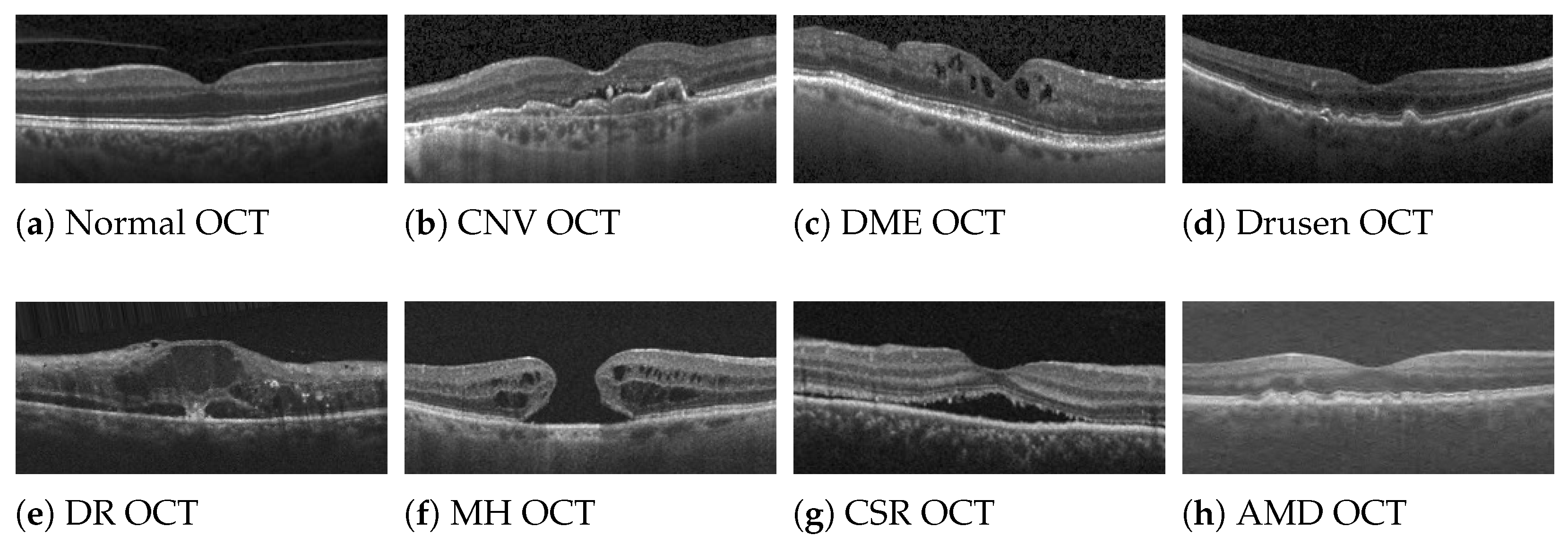
Figure 1 illustrates the eight retinal pathologies analyzed in this study, each presenting distinct morphological characteristics on OCT imaging. Normal OCT scans serve as the control group, displaying intact retinal layers including the retinal pigment epithelium (RPE), photoreceptor layers, and choroid without pathological alterations. Choroidal neovascularization (CNV) represents abnormal blood vessel proliferation from the choroid through Bruch’s membrane, commonly associated with wet AMD and characterized by subretinal fluid, hemorrhage, and fibrovascular tissue. Diabetic macular edema (DME) results from chronic hyperglycemia-induced retinal vascular damage, leading to increased capillary permeability and subsequent intraretinal fluid accumulation, typically appearing as cystoid spaces within retinal layers.

Drusen are extracellular deposits that accumulate between the RPE and Bruch’s membrane, representing early signs of AMD and appearing as dome-shaped elevations beneath the RPE. Diabetic retinopathy (DR) encompasses a spectrum of retinal vascular complications from diabetes, including microaneurysms, hemorrhages, hard exudates, and cotton wool spots, progressing from mild nonproliferative to severe proliferative stages. Macular holes (MH) are full-thickness defects in the neurosensory retina at the fovea, often idiopathic in origin and requiring surgical intervention to prevent permanent central vision loss. Central serous retinopathy (CSR) involves focal leakage from the choriocapillaris through the RPE, creating serous retinal detachment primarily affecting the macula and often associated with stress or corticosteroid use. Finally, age-related macular degeneration (AMD) represents the advanced form of macular degeneration, characterized by geographic atrophy (dry AMD) or choroidal neovascularization (wet AMD), leading to progressive central vision impairment.

2.1. Dataset Collection and Integration

The initial phase of the project involved collecting a random selection of OCT scans from two distinct datasets: Dataset #1 [32] (based on the original dataset [33] with duplicates removed) and Dataset #2 [34]. This approach was designed to increase the total number of cases and enhance variability across samples, thereby minimizing the risk of model overfitting during the training process. Around 3000 images of 8 pathologies were randomly selected to make certain there was an equal representation of each pathology in the model training. For the CNN and DNN models, these two datasets were split into training, test, and validation subgroups, with 70%, 15%, and 15% of images being allocated to each subgroup, respectively. For the Pycaret model, the dataset was split into only training and test datasets (70% and 30%, respectively) since Pycaret produces an internal validation dataset. After training, internal validating, and internal testing, an external dataset [35] was then acquired to observe the capabilities of the CNN and DNN models on unseen data (Figure 2). Pycaret was once again singled out due to difficulty obtaining the needed graphic results.

2.2. Data Preparation and Dataset Partitioning

The experimental pipeline commenced with the aggregation of optical coherence tomography (OCT) images from two primary datasets to enhance sample diversity and mitigate potential overfitting during model training [36]. Approximately 3000 images representing eight distinct retinal pathologies were randomly selected to ensure balanced class representation across the combined dataset.

The dataset partitioning process was implemented using a stratified random splitting algorithm to maintain class balance across training, validation, and test subsets. The splitting ratios were set to 70%, 15%, and 15%, respectively, following established best practices in machine learning for medical imaging applications. The detailed partitioning procedure is outlined in Algorithm 1.

Algorithm 1 Dataset Splitting Algorithm

1: for each class c in dataset do   2:     ${\mathrm{images}}_c\leftarrow$ list of images for class c   3:     $\mathrm{shuffle}\left({\mathrm{images}}_c\right)$   4:     $n_c\leftarrow \left|{\mathrm{images}}_c\right|$   5:     $\mathrm{train\_cutoff}\leftarrow \lfloor 0.7\times n_c\rfloor$   6:     $\mathrm{val\_cutoff}\leftarrow \lfloor 0.85\times n_c\rfloor$   7:     ${\mathrm{train\_set}}_c\leftarrow {\mathrm{images}}_c[0:\mathrm{train\_cutoff}]$   8:     ${\mathrm{val\_set}}_c\leftarrow {\mathrm{images}}_c[\mathrm{train\_cutoff}:\mathrm{val\_cutoff}]$   9:     ${\mathrm{test\_set}}_c\leftarrow {\mathrm{images}}_c[\mathrm{val\_cutoff}:n_c]$ 10:     Copy images to respective directories 11: end for

This stratified approach ensures that each pathology class maintains proportional representation across all data splits, thereby preserving the statistical properties of the original dataset distribution.

2.3. Model Selection and Methodological Focus

To provide a comprehensive comparative analysis, this study evaluated three distinct classes of machine learning models: (1) classical algorithms using an automated machine learning (AutoML) framework, (2) standard Convolutional Neural Networks (CNNs) trained from scratch, and (3) a Deep Neural Network (DNN) classifier built on pre-trained features. The following sections detail the implementation pipeline for each approach.

2.3.1. Automated ML Screening (PyCaret)

An initial baseline was established by screening 14 classical machine learning algorithms using the PyCaret AutoML library (version 3.3.2). This approach leveraged the same high-dimensional feature vectors used for the DNN model. Specifically, features were extracted from all images using the pre-trained VGG16 network (as detailed in Section 2.5) to produce a feature set of 25,088 dimensions per image. The dataset, comprising these feature vectors and their corresponding labels, was partitioned into a 70% training set and a 30% test set. PyCaret’s compare_models function was then executed on the training data, which automatically trained, cross-validated, and ranked all algorithms based on key performance metrics, with accuracy serving as the primary sorting criterion.

2.3.2. Convolutional Neural Networks (CNNs) Without Transfer Learning

To evaluate a common deep learning approach without transfer learning, a standard CNN was implemented in PyTorch (version 2.9.0) and trained from scratch. The architecture was designed to be straightforward and consisted of the following layers:

• A convolutional layer with 32 filters (3 × 3 kernel) and ReLU activation, followed by 2 × 2 max-pooling.
• A second convolutional layer with 64 filters (3 × 3 kernel) and ReLU activation, followed by 2 × 2 max-pooling.
• A fully connected layer with 512 units and ReLU activation.
• A final fully connected output layer with units corresponding to the number of pathology classes.

All models were trained for 10 epochs using the Adam optimizer (learning rate = 0.001), cross-entropy loss, and a batch size of 32. All input images were resized to 224 × 224 pixels and normalized (mean = [0.5, 0.5, 0.5], std = [0.5, 0.5, 0.5]). Two variants of this model were evaluated to assess the impact of data augmentation:

• CNN without Augmentation: This model was trained on images that underwent only resizing and normalization.
• CNN with Augmentation: For this variant, the training dataset was augmented using RandomHorizontalFlip, RandomRotation(10), and ColorJitter (brightness = 0.2, contrast = 0.2) transformations prior to resizing and normalization. The validation and test sets were not augmented for either model.

2.3.3. Deep Neural Network (DNN) with Pre-Trained Feature Extraction

The final and most successful modeling approach utilized a DNN classifier built upon features extracted from a pre-trained VGG16 network. This methodology, which is the primary focus of this paper due to its superior generalization performance and clinical applicability, is detailed in the subsequent Section 2.4, Section 2.5, Section 2.6 and Section 2.7. This approach was prioritized as it demonstrated the most robust and clinically reliable behavior, characterized by healthy learning dynamics and a monotonic decrease in performance across all data splits, which are critical prerequisites for clinical deployment.

This work prioritizes ML models with demonstrated real-world clinical applicability over architectural novelty. The detailed methodological framework employed here (i.e., encompassing detailed analysis of learning dynamics, multi-split validation, and external generalization assessment) directly serves this clinical objective. VGG16, extensively used in medical imaging research for its straightforward architecture and established reliability in transfer learning applications, provides stable and well-validated feature representations particularly appropriate for clinical contexts where consistency and interpretability are necessary. This architectural choice enabled focused evaluation of generalization behavior and training dynamics (i.e., critical prerequisites for clinical deployment) without introducing confounding variables associated with novel or complex architectures whose clinical reliability remains unproven.

2.4. Image Preprocessing and Data Loading Pipeline

All OCT images underwent standardized preprocessing to ensure compatibility with the VGG16 architecture requirements [36]. The preprocessing pipeline implemented the following transformations:

$$\begin{array}{cc}\hfill {\mathbf{I}}_{\mathrm{resized}}& =\mathrm{Resize}({\mathbf{I}}_{\mathrm{raw}},224\times 224),\hfill \\ \hfill {\mathbf{I}}_{\mathrm{tensor}}& =\mathrm{ToTensor}\left({\mathbf{I}}_{\mathrm{resized}}\right),\hfill \\ \hfill {\mathbf{I}}_{\mathrm{normalized}}& ={\displaystyle \frac{{\mathbf{I}}_{\mathrm{tensor}}-\mathit{\mu }}{\mathit{\sigma }}},\hfill \end{array}$$

(1)

where $\mathit{\mu }=[0.485,0.456,0.406]$ and $\mathit{\sigma }=[0.229,0.224,0.225]$ represent the ImageNet normalization parameters for RGB channels, respectively. This normalization ensures optimal feature extraction performance when using pre-trained ImageNet weights.

The data loading mechanism utilized PyTorch’s ImageFolder and DataLoader utilities with a batch size of 32 and shuffling enabled for all dataset splits to prevent ordering bias during training.

2.5. Feature Extraction Using Pre-Trained VGG16

A pre-trained VGG16 convolutional neural network served as a fixed feature extractor, leveraging transfer learning principles to obtain high-dimensional feature representations of the OCT images. The feature extraction process involved loading pre-trained weights and freezing all network parameters to prevent weight updates during subsequent training phases.

The VGG16 feature extractor architecture can be mathematically represented as:

$${\mathbf{f}}_i={\mathrm{VGG}16}_{\mathrm{features}}\left({\mathbf{I}}_i\right)$$

(2)

where ${\mathbf{I}}_i$ represents the i-th preprocessed input image and ${\mathbf{f}}_i\in {\mathbb{R}}^{25,088}$ denotes the corresponding flattened feature vector extracted from the final convolutional and pooling layers. The feature extraction module was implemented as described in Algorithm 2.

Algorithm 2 VGG16 Feature Extraction

1: Load pre-trained VGG16 weights from checkpoint   2: $\mathrm{vgg}16\leftarrow \mathrm{VGG}16(\mathrm{weight\_path})$   3: for param in vgg16.parameters() do   4:     param.requires_grad ← False   5: end for   6: Define feature extractor: $\mathrm{features}\circ \mathrm{avgpool}\circ \mathrm{flatten}$   7: for each dataloader in {train, val, test} do   8:     for batch in dataloader do   9:         $\mathbf{features}\leftarrow \mathrm{features\_extractor}(\mathrm{batch})$ 10:         Store features and labels 11:     end for 12: end for

2.6. Deep Neural Network Classifier Architecture

The extracted VGG16 features served as input to a fully connected deep neural network (DNN) classifier designed for multi-class pathology classification. The DNN architecture comprised the following layers:

• Input layer: 25,088 units (matching VGG16 feature dimensionality)
• Hidden layer: 256 units with ReLU activation function
• Dropout layer: $p=0.3$ for regularization
• Output layer: C units (where C is the number of pathology classes)

The forward propagation through the DNN can be expressed mathematically as:

$$\begin{array}{cc}\hfill \mathbf{h}& =\mathrm{ReLU}({\mathbf{W}}_1\mathbf{f}+{\mathbf{b}}_1),\hfill \\ \hfill {\mathbf{h}}^{\prime }& =\mathrm{Dropout}(\mathbf{h},p=0.3),\hfill \\ \hfill \mathbf{o}& ={\mathbf{W}}_2{\mathbf{h}}^{\prime }+{\mathbf{b}}_2,\hfill \end{array}$$

(3)

where ${\mathbf{W}}_1\in {\mathbb{R}}^{256\times 25,088}$ and ${\mathbf{b}}_1\in {\mathbb{R}}^{256}$ represent the weights and biases of the hidden layer, while ${\mathbf{W}}_2\in {\mathbb{R}}^{C\times 256}$ and ${\mathbf{b}}_2\in {\mathbb{R}}^C$ correspond to the output layer parameters.

2.7. Training Methodology and Optimization

The DNN classifier was trained using the Adam optimization algorithm with a learning rate of $\alpha =0.001$. The training objective utilized the multi-class cross-entropy loss function:

$$\mathcal{L}(\mathbf{y},\widehat{\mathbf{y}})=-{\displaystyle \frac{1}{N}}\sum _{i=1}^N\sum _{c=1}^C{y}_{ic}log\left(\mathrm{softmax}\left(o_{ic}\right)\right),$$

(4)

where $y_{ic}$ is the binary indicator (0 or 1) representing whether class label c is correct for sample i, and $o_{ic}$ represents the raw output logit for class c and sample i. The training loop was executed for 10 epochs, with each epoch consisting of the operations detailed in Algorithm 3.

Algorithm 3 DNN Training Loop

1: for epoch = 1 to num_epochs do   2:     classifier.train()   3:     optimizer.zero_grad()   4:     $\mathbf{outputs}\leftarrow \mathrm{classifier}\left(\mathbf{train\_features}\right)$   5:     $\mathcal{L}\leftarrow \mathrm{CrossEntropyLoss}(\mathbf{outputs},\mathbf{train\_labels})$   6:     $\mathcal{L}.\mathrm{backward}\left(\right)$   7:     optimizer.step()   8:     Calculate training accuracy: ${\mathrm{acc}}_{\mathrm{train}}={\displaystyle \frac{{\sum }_{i=1}^N\mathbf{1}[argmax\left({\mathbf{o}}_i\right)=y_i]}{N}}$   9:     classifier.eval() 10:     $\mathbf{val\_outputs}\leftarrow \mathrm{classifier}\left(\mathbf{val\_features}\right)$ 11:     Calculate validation accuracy: ${\mathrm{acc}}_{\mathrm{val}}$ 12: end for

In ML training, the number of epochs should be determined by convergence behavior rather than arbitrary targets. Hence, the selection of 10 training epochs was determined through preliminary empirical testing and convergence monitoring rather than arbitrary convention. In ML, the optimal number of epochs is dataset- and architecture-specific, determined by observing when validation performance stabilizes rather than adhering to predetermined iteration counts. Preliminary experiments indicated that convergence typically occurred within 8–10 epochs for this dataset and architecture combination, with validation accuracy plateauing and minimal improvement observed beyond this point.

The use of pre-trained VGG16 features as fixed representations (Section 2.5) substantially reduced the epochs required for convergence compared to end-to-end training approaches. Since only the classifier head trains on high-level feature embeddings rather than learning convolutional filters from random initialization, the optimization landscape is considerably simpler and convergence occurs more rapidly. Transfer learning approaches of this type typically achieve convergence within 5–15 epochs depending on dataset complexity and classifier architecture. Training beyond observed convergence risks overfitting, where the model begins memorizing training-specific patterns rather than learning generalizable features, potentially manifesting as widening train-validation performance gaps.

2.8. Model Evaluation and Performance Metrics

Detailed model evaluation was conducted across training, validation, and test datasets using multiple performance metrics and diagnostic tools [36]. The evaluation framework comprised two primary components: learning dynamics analysis through learning curves and subset-wise performance assessment across data splits.

2.8.1. Learning Dynamics and Learning Curve Analysis

Learning curves served as the primary diagnostic tool for assessing model training dynamics and identifying potential issues such as overfitting, underfitting, or convergence instability. Learning curves were generated by plotting both training and validation accuracy as functions of training epochs:

$$\begin{array}{cc}\hfill {\mathcal{C}}_{\mathrm{train}}\left(e\right)& ={\displaystyle \frac{1}{N_{\mathrm{train}}}}\sum _{i=1}^{N_{\mathrm{train}}}\mathbf{1}[argmax\left(f_{{\theta }_e}\left({\mathbf{x}}_i\right)\right)=y_i],\hfill \\ \hfill {\mathcal{C}}_{\mathrm{val}}\left(e\right)& ={\displaystyle \frac{1}{N_{\mathrm{val}}}}\sum _{j=1}^{N_{\mathrm{val}}}\mathbf{1}[argmax\left(f_{{\theta }_e}\left({\mathbf{x}}_j^{\mathrm{val}}\right)\right)=y_j^{\mathrm{val}}],\hfill \end{array}$$

(5)

where ${\mathcal{C}}_{\mathrm{train}}\left(e\right)$ and ${\mathcal{C}}_{\mathrm{val}}\left(e\right)$ represent the training and validation accuracies at epoch e, respectively, $f_{{\theta }_e}$ denotes the model with parameters $\theta$ at epoch e, and $\mathbf{1}[·]$ is the indicator function.

Learning curve analysis provided insights into model behavior throughout the training process. Healthy learning curves were characterized by several key features: (1) Parallel convergence: Both training and validation curves should exhibit similar upward trajectories without excessive divergence, indicating that the model generalizes well to unseen data [36]. (2) Smooth progression: Curves should demonstrate steady improvement without erratic fluctuations, suggesting stable gradient-based optimization. (3) Appropriate convergence gap: A small, consistent gap between training and validation performance is expected, with training accuracy typically slightly exceeding validation accuracy [36].

Conversely, several problematic learning patterns can be identified in training dynamics, each indicating specific underlying issues if observed. Overfitting signatures would manifest as rapid training accuracy saturation (approaching 100%) while validation accuracy plateaus at significantly lower levels, creating widening performance gaps [36]. Such behavior would suggest that the model is memorizing training examples rather than learning generalizable patterns. Validation instability would be characterized by erratic fluctuations in the validation curve, particularly after initial epochs, indicating that the model is becoming increasingly specialized to the training data rather than learning robust features that transfer to unseen data. Premature saturation would occur when training accuracy reaches maximum values early in training while validation performance stagnates, signaling memorization rather than meaningful pattern learning [36].

The learning curve generation process was implemented through epoch-wise accuracy computation during the training loop [36]:

• At each training epoch e, compute training accuracy using current model parameters
• Evaluate model on validation set using identical parameters (without gradient updates)
• Store accuracy values: $\{{\mathcal{C}}_{\mathrm{train}}\left(1\right),{\mathcal{C}}_{\mathrm{train}}\left(2\right),\dots ,{\mathcal{C}}_{\mathrm{train}}\left(E\right)\}$ and $\{{\mathcal{C}}_{\mathrm{val}}\left(1\right),{\mathcal{C}}_{\mathrm{val}}\left(2\right),\dots ,{\mathcal{C}}_{\mathrm{val}}\left(E\right)\}$
• Generate visualization plotting both curves against epoch number
• Analyze curve patterns for training dynamic assessment

2.8.2. Subset-Wise Performance Dynamics

Beyond learning curves, detailed evaluation requires a systematic assessment of model performance across all data splits to understand generalization behavior and detect potential data-related issues. Subset-wise performance dynamics involves computing performance metrics across all available data partitions, including internal splits (training, validation, test) and external validation datasets when available [36]. This multi-tiered evaluation framework enables the detection of generalization failures and provides insights into model robustness across different data exposure scenarios.

The primary evaluation metrics were computed consistently across all subsets:

$$\begin{array}{cc}\hfill \mathrm{Accuracy}& ={\displaystyle \frac{\mathrm{TP}+\mathrm{TN}}{\mathrm{TP}+\mathrm{TN}+\mathrm{FP}+\mathrm{FN}}},\hfill \\ \hfill \mathrm{Precision}& ={\displaystyle \frac{\mathrm{TP}}{\mathrm{TP}+\mathrm{FP}}},\hfill \\ \hfill \mathrm{Recall}& ={\displaystyle \frac{\mathrm{TP}}{\mathrm{TP}+\mathrm{FN}}},\hfill \\ \hfill \mathrm{F}1\text{-}\mathrm{Score}& =2\times {\displaystyle \frac{\mathrm{Precision}\times \mathrm{Recall}}{\mathrm{Precision}+\mathrm{Recall}}},\hfill \end{array}$$

(6)

where TP, TN, FP, and FN represent true positives, true negatives, false positives, and false negatives, respectively, computed for each data subset independently.

Expected performance patterns follow predictable hierarchical trends for well-generalizing models. Performance typically achieves maximum values on the training set, demonstrates moderate decline on the validation set, exhibits further modest reduction on the test set, and shows additional decline on external datasets. This monotonic decrease pattern: ${\mathrm{Performance}}_{\mathrm{train}}\ge {\mathrm{Performance}}_{\mathrm{val}}\ge {\mathrm{Performance}}_{\mathrm{test}}\ge {\mathrm{Performance}}_{\mathrm{external}}$ serves as a fundamental indicator of appropriate model generalization. Anomalous performance patterns signal potential methodological issues requiring investigation. Non-monotonic improvements, where validation or test performance exceeded training performance, suggested possible data leakage, inappropriate data splitting, or extremely small dataset sizes leading to statistical artifacts. Excessive performance gaps between training and validation/test sets indicated overfitting, while unusually small gaps might suggest underfitting or data insufficiency. Dramatic performance drops between internal (train/val/test) and external validation sets could indicate distribution shift, dataset bias, or poor model generalizability to real-world conditions.

Performance increases on external test sets, while superficially appearing favorable, typically represent significant methodological concerns. Such unexpected improvements could indicate several problematic scenarios: (1) Fortuitous dataset characteristics, where the external dataset inadvertently contains easier-to-classify cases or exhibits reduced inter-class variability compared to internal splits. (2) Evaluation inconsistencies, where different preprocessing procedures, class distributions, or scoring methodologies between internal and external validation create artificial performance improvements. (3) Data leakage, where information from the external dataset inadvertently influenced model development through hyperparameter tuning or architectural decisions. (4) Distribution shift favoring the model, where the external dataset’s characteristics align more closely with the model’s learned representations than the original training distribution, creating an unrepresentative assessment of true generalization capability.

The subset-wise evaluation protocol was implemented systematically:

• Extract features for all data splits: ${\mathbf{F}}_{\mathrm{train}},{\mathbf{F}}_{\mathrm{val}},{\mathbf{F}}_{\mathrm{test}}$
• Train classifier exclusively on ${\mathbf{F}}_{\mathrm{train}}$ with corresponding labels
• Evaluate trained model on each subset independently:

  (a)

  Forward pass: ${\mathbf{o}}_s=\mathrm{classifier}\left({\mathbf{F}}_s\right)$ for subset $s\in \{\mathrm{train},\mathrm{val},\mathrm{test}\}$

  (b)

  Compute probabilities: ${\mathbf{p}}_s=\mathrm{softmax}\left({\mathbf{o}}_s\right)$

  (c)

  Generate predictions: ${\widehat{\mathbf{y}}}_s=argmax\left({\mathbf{p}}_s\right)$

  (d)

  Calculate all metrics using true labels ${\mathbf{y}}_s$ and predictions ${\widehat{\mathbf{y}}}_s$

• Compare metric values across subsets for pattern analysis
• Generate confusion matrices for detailed class-specific performance assessment

Additionally, confusion matrices were generated for each dataset split to provide detailed insight into class-specific classification performance and error patterns. The confusion matrix $\mathbf{C}$ for subset s was computed as:

$${\mathbf{C}}_{ij}^{\left(s\right)}=\sum _{k=1}^{N_s}\mathbf{1}[y_k^{\left(s\right)}=i\mathrm{and}{\widehat{y}}_k^{\left(s\right)}=j],$$

(7)

where ${\mathbf{C}}_{ij}^{\left(s\right)}$ represents the count of samples with true label i predicted as label j in subset s.

This detailed evaluation framework enables thorough assessment of model reliability, generalization capability, and potential methodological concerns through both temporal learning dynamics and cross-subset performance consistency analysis.

2.9. Implementation Framework and Computational Resources

The entire experimental pipeline was implemented in Python 3.14 using the PyTorch deep learning framework for neural network operations and scikit-learn for evaluation metrics. Computational resources included CUDA-enabled GPU acceleration when available, with automatic fallback to CPU processing. Random seed initialization ensured reproducibility across experimental runs.

The complete experimental workflow can be summarized as:

• Dataset aggregation and stratified splitting
• Image preprocessing and normalization
• VGG16 feature extraction with frozen weights
• DNN classifier training on extracted features
• Comprehensive evaluation across multiple metrics
• External validation on independent test dataset

This methodology ensures a detailed and reproducible approach to DNN training for multi-class OCT pathology classification, with careful attention to data integrity, model architecture design, and comprehensive performance evaluation.

2.10. Prerequisite for Clinical Translation

Critically, without systematic assessment of learning dynamics, no ML study’s results can be considered scientifically reliable or clinically relevant, as learning curves serve as the fundamental diagnostic tool for distinguishing between models that have learned generalizable patterns versus those that have merely memorized training data.

This distinction becomes vital in healthcare applications, where overfitted models that appear to perform exceptionally well on internal validation may fail when deployed on real patients from different populations, institutions, or acquisition protocols. The healthcare ML literature is particularly vulnerable to reporting inflated performance metrics that mask underlying overfitting or data leakage issues. Many studies delineate only summary statistics without the learning dynamics evidence necessary to validate that their models possess true generalization capability.

Consequently, any ML model intended for medical deployment must demonstrate through learning curve analysis that its training and validation performance converge in a stable, parallel manner without the telltale signs of overfitting such as rapid training saturation, widening train-validation gaps, or validation instability.

Table 1. Vital criteria for evaluating ML model generalizability in clinical applications. This checklist enables assessment of study rigor and model reliability for patient safety.

Evaluation Criterion	Healthy Pattern/Good Practice	Warning Signs/Poor Practice
Learning Curve Dynamics	Parallel, smooth convergence of training and validation curves with minimal gap	Rapid training saturation, widening train-validation gaps, validation instability
Performance Across Splits	Monotonic decrease: Train ≥ Val ≥ Test ≥ External	Non-monotonic improvements, dramatic performance drops, missing external validation
Training Progression	Steady, gradual improvement over epochs with stable convergence	Early saturation, erratic fluctuations, validation performance decline
Overfitting Assessment	Small, consistent train-validation gap (<5–10%) throughout training	Large gaps (>20%), validation plateau while training continues improving
Data Split Methodology	Stratified random splits with proper temporal/institutional separation	Unclear splitting procedures, potential data leakage, inadequate split documentation
External Validation	Independent dataset from different institution/population with expected performance decline	Missing external validation, unexpectedly high external performance, same-source external data
Metric Consistency	Consistent reporting across all splits with multiple complementary metrics	Cherry-picked metrics, single-split reporting, missing confusion matrices
Reproducibility Documentation	Detailed methodology, hyperparameters, random seeds, code availability	Insufficient detail for reproduction, missing implementation specifics

provides a detailed checklist of essential criteria for evaluating ML model generalizability in clinical applications, enabling systematic assessment of study rigor and model reliability [36].

Models that fail to exhibit healthy learning dynamics, regardless of their reported accuracy metrics, represent a fundamental threat to patient safety and should be disqualified from clinical consideration, as their apparent success likely reflects memorization of dataset idiosyncrasies rather than acquisition of clinically relevant diagnostic patterns that will reliably transfer to unseen patients in real-world deployment scenarios.

3. Results

The experimental workflow consisted of two main stages. Initially, a range of classical ML algorithms was screened using PyCaret to establish a rapid performance baseline and to facilitate automated model selection. Following this, the focus shifted to custom image-based models implemented in Python, including a CNN without augmentation, a CNN with augmentation, and a fully connected DNN. This sequential approach enabled both a broad comparison of algorithmic strategies and a more controlled investigation of neural network architectures for image classification. The rationale for transitioning from PyCaret to custom neural network models was to allow for more detailed control over training dynamics and to address limitations observed in the automated pipeline. The results of each stage are presented in the following sections.

3.1. Automated Model Screening (PyCaret)

Table 2. PyCaret model performance comparison on internal cross-validation. Models are ranked by accuracy with corresponding performance metrics across multiple evaluation criteria.

Model 1	Accuracy	AUC	Recall	Prec.	F1	Kappa	MCC
lightgbm	0.9101	0.9917	0.9101	0.9106	0.9102	0.8972	0.8973
lr	0.8921	0.0000	0.8921	0.8925	0.8921	0.8765	0.8766
lda	0.8878	0.0000	0.8878	0.8908	0.8881	0.8717	0.8720
svm	0.8831	0.0000	0.8831	0.8896	0.8815	0.8663	0.8679
ridge	0.8831	0.0000	0.8831	0.8844	0.8829	0.8663	0.8665
et	0.8729	0.9848	0.8729	0.8745	0.8723	0.8547	0.8551
gbc	0.8722	0.0000	0.8722	0.8730	0.8722	0.8539	0.8540
rf	0.8686	0.9847	0.8686	0.8696	0.8681	0.8497	0.8500
qda	0.8555	0.0000	0.8555	0.8623	0.8560	0.8346	0.8358
knn	0.8523	0.9696	0.8523	0.8595	0.8518	0.8311	0.8323
nb	0.7091	0.9485	0.7091	0.7314	0.7090	0.6677	0.6715
dt	0.6542	0.8015	0.6542	0.6553	0.6543	0.6044	0.6046
ada	0.4352	0.0000	0.4352	0.4520	0.4210	0.3545	0.3608
dummy	0.1425	0.5000	0.1425	0.0203	0.0356	0.0000	0.0000

¹ Model abbreviations: lightgbm = Light Gradient Boosting Machine; lr = Logistic Regression; lda = Linear Discriminant Analysis; svm = SVM-Linear Kernel; ridge = Ridge Classifier; et = Extra Trees Classifier; gbc = Gradient Boosting Classifier; rf = Random Forest Classifier; qda = Quadratic Discriminant Analysis; knn = K Neighbors Classifier; nb = Naive Bayes; dt = Decision Tree Classifier; ada = Ada Boost Classifier; dummy = Dummy Classifier.

summarizes PyCaret’s internal cross-validation ranking across 14 different machine learning algorithms. The Light Gradient Boosting Machine (lightgbm) achieved the highest cross-validation accuracy of 91.01% with an exceptionally high AUC of 0.9917, demonstrating strong discriminative capability. However, a substantial performance gap exists between the top-performing model and the second-ranked Logistic Regression (lr) at 89.21% accuracy. The top-tier models (lightgbm, lr, lda, svm, ridge) all demonstrate remarkably consistent performance across metrics, with accuracy, recall, precision, and F1-scores varying by less than 0.01, suggesting balanced classification performance across all disease categories.

Notably, several models show AUC values of 0.0000, likely indicating that multiclass AUC computation was not performed for these algorithms in PyCaret’s automated pipeline. The ensemble methods (lightgbm, et, rf) that do report AUC values consistently achieve scores above 0.98, confirming their strong ranking discrimination. Performance degrades substantially in the lower-ranked models, with Ada Boost Classifier achieving only 43.52% accuracy and the Dummy Classifier baseline at 14.25%.

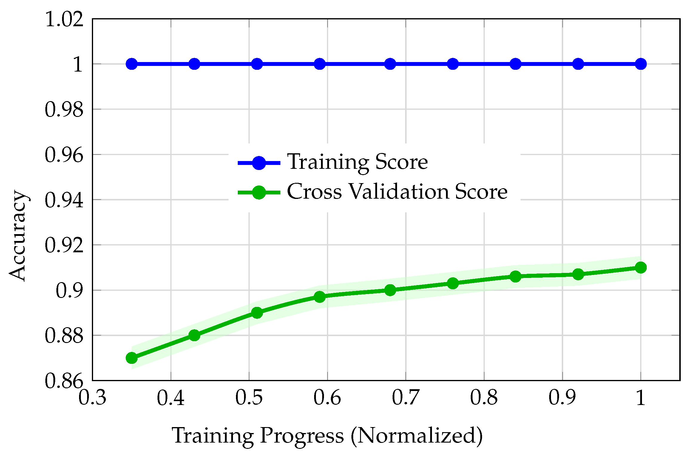
Despite LightGBM’s superior cross-validation metrics, its learning curves (Figure 3) revealed problematic training dynamics indicative of overfitting or data leakage: training performance increased while validation performance plateaued and diverged rather than improving commensurately. This unfavorable train-validation behavior, characterized by early validation stagnation despite continued training improvement, rendered the model unsuitable for reliable generalization. Consequently, we did not advance any PyCaret models to external validation, instead focusing on custom-implemented neural network architectures for more controlled training dynamics.

3.2. Convolutional Neural Networks (CNNs)

This section evaluates the performance and learning behavior of CNNs, both with and without data augmentation. The following subsections provide a side-by-side analysis of learning dynamics for each model variant. First, “CNN without augmentation” details the training and validation accuracy curves for the unaugmented model, highlighting characteristic signs of overfitting and instability. Next, “CNN with augmentation” examines how introducing augmentation affects convergence and generalization, identifying both improvements and remaining concerns. Together, these analyses clarify the impact of augmentation on CNN robustness and help interpret the reliability and limitations of each model’s results.

3.2.1. CNN Without Augmentation

The unaugmented CNN exhibits severe overfitting with multiple red flags: (1) Rapid training saturation: training accuracy climbs aggressively from 70% to nearly 100% within the first half of training, indicating the model is memorizing rather than learning generalizable patterns; (2) Large train-validation gap: validation accuracy plateaus around 79% while training continues to 100%, creating a 21-point performance gap that signals poor generalization; (3) Validation instability: the validation curve shows concerning fluctuations after epoch 4, including a notable dip around epoch 8, suggesting the model is becoming increasingly specialized to the training set. This pattern is characteristic of classical overfitting where increased training time paradoxically worsens generalization performance.

3.2.2. CNN with Augmentation

The augmented CNN shows dramatically improved training dynamics: both curves start at realistic baseline performance (∼47%) and converge smoothly with minimal train-validation gap. However, one subtle red flag emerges: validation accuracy slightly exceeds training accuracy at the end (84.5% vs. 86%), which, while small, is theoretically unexpected since validation data is never seen during parameter updates. This could indicate: (1) fortunate data split where validation happens to be slightly easier, (2) regularization effects from augmentation that benefit validation more than training, or (3) subtle evaluation inconsistencies. Despite this minor concern, the augmented model demonstrates healthy learning dynamics with steady, parallel improvement on both splits.

3.3. Deep Neural Network (DNN)

This section presents a detailed evaluation of the DNN model, focusing on its learning behavior and generalization performance. First, the “Learning dynamics” examines the progression of training and validation accuracy across epochs to assess whether the DNN exhibits stable and robust learning. Next, the “Per-split performance and diagnostics” provides confusion matrices and summary metrics for the training, validation, and test sets, enabling a granular analysis of classification strengths and weaknesses across classes. Together, these analyses offer a detailed view of the DNN’s reliability and diagnostic value across all data splits.

3.3.1. Learning Dynamics

Figure 4 displays the learning curves for the DNN model. Both training and validation accuracy increase steadily across epochs, with no abrupt divergence or instability. This parallel progression closely mirrors the healthy learning dynamics observed in the augmented CNN (see Figure 5), where both curves also converge smoothly with minimal gap. In both cases, the stable, near-parallel trajectories indicate effective generalization and robust learning, distinguishing these models from the regular CNN and LightGBM, which exhibited overfitting or implausible dynamics.

3.3.2. Per-Split Performance and Diagnostics

Figure 6 provides confusion matrices for the DNN across the training, validation, and test sets, accompanied by summary performance metrics. The matrices reveal the distribution of correct and incorrect predictions for each class, with most errors concentrated in specific off-diagonal entries. The accompanying metrics—accuracy, precision, recall, and F1-score—are reported for each split, demonstrating the DNN’s consistent performance and highlighting areas of class confusion.

A detailed examination of the confusion matrices in Figure 6 reveals several consistent patterns in the DNN’s classification behavior across the training, validation, and test sets. For most classes, the majority of predictions are concentrated along the diagonal, indicating correct classification. However, certain classes exhibit persistent off-diagonal confusion, highlighting specific areas where the model struggles.

Class 1 (Normal) is classified with near-perfect accuracy across all splits, with negligible misclassification into class 2 (CNV) and no confusion with other classes. In contrast, class 2 (CNV) shows a recurring pattern of misclassification into class 6 (MH), with 18.0%, 17.1%, and 14.7% of class 2 (CNV) samples in the training, validation, and test sets, respectively, being incorrectly labeled as class 6 (MH). This suggests a substantial overlap in the feature representations of these two classes, which the model is unable to fully disentangle.

Class 3 (DME) is generally well-classified, but a notable proportion of its samples are misassigned to classes 5 (DR) and 7 (CSR), with 4.0–5.8% going to class 5 (DR) and 7.1–8.2% to class 7 (CSR) across splits. This indicates moderate ambiguity between these classes, though the majority of class 3 (DME) samples are still correctly identified.

Class 4 (Drusen) stands out as the most challenging for the model, with less than half of its samples correctly classified (46.7% train, 48.2% validation, 34.1% test). The most frequent misclassifications for class 4 (Drusen) are into classes 2 (CNV), 6 (MH), and 8 (AMD), with off-diagonal rates as high as 25.5% (train, into class 8 (AMD)) and 22.2% (validation, into class 8 (AMD)). This persistent confusion suggests that class 4 (Drusen) shares substantial feature similarity with these other classes, or that it is underrepresented or more heterogeneous in the dataset. Thus, this misclassification reflects the underlying clinical relationship between drusen and these retinal pathologies. Drusen are extracellular deposits that accumulate between the retinal pigment epithelium and Bruch’s membrane, and their presence exists on a clinicopathological spectrum. While a few small (hard) drusen are considered a normal aging change, the accumulation of larger and more numerous drusen represents the pathological hallmark of early age-related macular degeneration. Importantly, drusen are not merely associated with AMD; they are an integral component of the disease process itself, with large confluent drusen representing pathological signs rather than benign age-related changes.

This creates a fundamental classification challenge: images labeled as “Drusen” (Class 4) often contain significant drusen burden that is clinically indistinguishable from early-stage AMD (Class 8), since substantial drusen accumulation is itself a manifestation of AMD pathology. Similarly, drusen presence substantially increases the risk of progression to choroidal neovascularization, the defining feature of wet AMD, creating feature overlap between Class 4 (Drusen) and Class 2 (CNV). The model’s frequent confusion among these classes therefore reflects genuine clinical ambiguity in the continuum from normal aging to drusen accumulation to advanced macular degeneration, rather than pure classification error. OCT images showing prominent drusen may legitimately belong to multiple disease categories depending on additional clinical context not captured in the imaging alone, making this a boundary where even expert human graders would demonstrate inter-rater variability.

Classes 5 (DR) and 7 (CSR) are classified with high accuracy (over 90% correct in all splits), with only minor confusion into neighboring classes (e.g., class 5 (DR) into class 3 (DME), class 7 (CSR) into class 5 (DR)). Class 6 (MH), however, is frequently confused with class 2 (CNV) (11.4–14.9% across splits) and class 8 (AMD) (10–12.5%), indicating that the model has difficulty distinguishing between these categories.

Finally, class 8 (AMD) is correctly classified in approximately 86% of cases, with the main errors being misclassification into class 6 (MH) (8.9–10.9%) and class 2 (CNV) (2.3–2.7%). This pattern is consistent across all splits, suggesting a stable but imperfect separation between these classes.

Overall, the confusion matrices demonstrate that while the DNN achieves strong overall performance, its errors are not randomly distributed but are concentrated among specific class pairs; most notably between classes 2 and 6, and among classes 4, 2, 6, and 8. These findings highlight the importance of targeted model improvements or data augmentation strategies for these challenging class boundaries.

3.4. External Validation

To enable a direct across-model comparison on the most challenging data, Figure 7 summarizes the performance of all evaluated models (regular CNN, augmented CNN, and DNN) across the train, validation, test, and external datasets. The figure plots accuracy, F1-score, precision, and recall for each model and split, enabling direct comparison of generalization behavior. The DNN shows a monotonic decrease in most metrics from internal to external evaluation, while the CNN variants display non-monotonic trends, particularly in the external set.

A monotonic decrease in performance metrics (i.e., accuracy, F1-score, precision, and recall) from the training set through validation, test, and finally to the external set is generally considered a hallmark of robust model generalization. This expectation arises from the increasing difficulty and unfamiliarity of each subsequent dataset. The training set is directly used for parameter optimization, so models typically achieve their highest performance there. The validation and test sets, while unseen during training, are often drawn from the same underlying distribution as the training data, so a modest drop in performance is expected as the model is evaluated on data it has not directly seen but is still similar in nature.

The external set, by contrast, is intended to represent the most challenging and realistic scenario for model deployment: it is ideally sourced independently and may differ in subtle or substantial ways from the training distribution (e.g., due to site, population, or acquisition differences). As a result, a further decrease in performance is desirable to observe, as it reflects the model’s ability to generalize to genuinely novel data. However, this decrease should not be excessively steep. A gradual, monotonic decline suggests that the model has learned generalizable patterns rather than memorizing idiosyncrasies of the training data. If the drop is too abrupt, it may indicate overfitting, data leakage, or a significant distributional mismatch between the training and external sets, all of which undermine the model’s practical utility.

4. Discussion

This discussion synthesizes the comparative findings from all evaluated models, focusing on learning dynamics, generalization patterns, and the interpretability of model performance across internal and external splits.

4.1. Key Observations and Takeaways

The comparative analysis of model performance across LightGBM (via PyCaret), regular CNN, augmented CNN, and DNN reveals distinct patterns in learning dynamics and generalization behavior. Although LightGBM achieved a strong cross-validation score (best CV accuracy: 91.0%), its learning curves (Figure 3) exposed problematic training dynamics. The training accuracy remained at 100% throughout, while cross-validation accuracy improved only marginally from 87.0% to 91.0%, with a persistent and widening gap between training and validation. This divergence, coupled with early stagnation of the validation curve, is indicative of overfitting or possible data leakage. Such behavior undermines confidence in the model’s ability to generalize, justifying the decision not to advance PyCaret models to external validation. The regular (unaugmented) CNN also exhibited severe overfitting (Figure 5). Training accuracy rapidly saturated at 100%, while validation accuracy plateaued at 79%, resulting in a substantial 21-point gap. The validation curve also displayed instability, with fluctuations and a notable dip around epoch 8, further signaling poor generalization and memorization of the training set rather than learning robust features.

In contrast, the augmented CNN demonstrated healthier learning dynamics. Both training and validation accuracies started at realistic baselines (47%) and converged smoothly, with the validation curve closely tracking the training curve and ending at 84.5% (validation) versus 86% (training). This small, expected gap, where training accuracy remains slightly higher than validation accuracy, reflects robust generalization and effective regularization. Overall, the augmented CNN’s learning curves were markedly better than both LightGBM and the regular CNN. The DNN’s learning curves (Figure 4) also showed smooth, parallel convergence of training and validation accuracy, with no abrupt divergence. Accuracy improved steadily from 37% to 80% (training) and from 29% to 75% (validation) over the training size.

Confusion matrices (Figure 6) revealed that most errors were concentrated among classes 2, 4, and 6, with notable off-diagonal confusion, especially for class 4, which had substantial misclassification into classes 2, 6, and 8. This pattern may reflect clinical or feature overlap among these categories.

When examining performance across splits (Figure 7), the DNN was the only model to exhibit the expected monotonic decrease in most performance metrics from training to validation to test to external. The only exception was precision, which increased on the external set; likely reflecting a more conservative prediction strategy in response to distributional shift, where the model made fewer positive predictions but with higher accuracy. In contrast, the augmented CNN showed non-monotonic improvement, with external set metrics (e.g., accuracy up to 90.5%, precision up to 92%) exceeding those on the test and even training sets. This is highly unusual and suggests either a mismatch in data splits, potential leakage, or that the external set was inadvertently easier for the model.

While such unexpectedly elevated external performance might initially appear favorable, it fundamentally contradicts the expected generalization hierarchy wherein models should demonstrate monotonically decreasing performance as data becomes increasingly unfamiliar. External validation datasets, by definition, originate from different sources with distinct acquisition protocols, patient populations, and imaging characteristics, thereby representing the most challenging evaluation scenario. When a model’s external performance paradoxically exceeds its internal validation or test performance, this anomaly typically indicates that the external dataset inadvertently simplified the classification task; whether through fortuitous class distributions that align with the model’s learned biases, systematically clearer image quality that facilitates feature extraction, exclusion of diagnostically ambiguous cases that challenged internal validation, or statistical artifacts arising from small sample sizes. Such performance improvements cannot be interpreted as evidence of superior generalization capability; rather, they signal that the external validation failed to provide a genuinely independent or representative assessment of real-world clinical performance. Consequently, models exhibiting non-monotonic performance patterns must be regarded with heightened skepticism regardless of their numerical metrics, as these results likely reflect evaluation artifacts or dataset peculiarities rather than reliable diagnostic competence that would translate to diverse clinical deployment scenarios.

The regular CNN, meanwhile, showed a dramatic drop from 100% training accuracy to 79% (validation), 78% (test), and as low as 73% (external), further confirming its overfitting and lack of generalization.

Building on these observations, the DNN’s performance metrics generally decreased gradually from training to validation to test to external sets, as expected for a well-generalizing model. Specifically, accuracy dropped from 82% (train) to 81.5% (validation), 81% (test), and 76% (external). F1-score followed a similar trend: 82% (train), 81.5% (validation), 81% (test), and 80.5% (external). Recall also decreased monotonically across splits. However, precision notably increased on the external set, rising from 84% on train to 86% on external. This counterintuitive trend suggests that the model became more conservative in its positive predictions when faced with new data. Such an increase in precision, especially when recall drops, often indicates that the model is making fewer positive predictions overall, but those it does make are more likely to be correct. This behavior is commonly observed when there is a distributional shift between training and external data, prompting the model to raise its internal threshold for positive classification. As a result, the model reduces false positives (increasing precision) at the expense of missing more true positives (lower recall), reflecting a typical trade-off in response to increased uncertainty or changes in data distribution.

To synthesize these findings,

Table 3. Summary of model training and generalization dynamics. A checkmark (✓) indicates the model satisfied the criterion; a cross (✗) indicates it did not.

Model	Healthy Learning Curves 1	Monotonic Decrease of Performance Metrics 2
LightGBM (PyCaret)	✗	✗
Regular CNN	✗	✗
Augmented CNN	✓	✗
DNN	✓	✓

¹ Healthy learning curves are defined as smooth, parallel convergence of training and validation accuracy without signs of overfitting or instability. ² Monotonic decrease refers to performance metrics (accuracy, F1, etc.) decreasing smoothly from training to external sets, without unexpected jumps or reversals.

summarizes how each model satisfied two key criteria: (1) exhibiting healthy learning curves, and (2) demonstrating a monotonic decrease in performance metrics across data splits. As shown, both LightGBM (via PyCaret) and the regular CNN failed to meet either criterion, reflecting their poor generalization and overfitting tendencies. The augmented CNN achieved healthy learning curves but did not maintain a monotonic decrease in performance metrics, primarily due to its unexpected improvement on both the test and external sets. Notably, only the DNN satisfied both criteria, highlighting its robust learning dynamics and consistent generalization behavior across all evaluation splits.

The DNN’s external validation accuracy of 76%, while representing a decline from internal performance metrics, warrants careful interpretation within the broader context of clinical ML development. First, the presence of external validation itself distinguishes this work from the majority of published OCT classification studies, which typically report only internal test set performance without independent dataset assessment. Second, the monotonic performance decrease from training (82%) through validation (81.5%), test (81%), to external validation (76%) represents a fundamental indicator of model reliability and methodological integrity. This gradual, consistent decline demonstrates that the model has learned generalizable patterns rather than memorizing dataset-specific artifacts. In contrast, models exhibiting inflated internal accuracies (approaching 95–100%) without external validation evidence, or those showing non-monotonic performance patterns, may achieve superficially impressive metrics while masking serious generalization failures that would only become apparent upon clinical deployment. The 76% external accuracy, though modest, provides an honest, conservative estimate of real-world performance expectations. Such transparency is essential for responsible clinical translation, as overestimating model capabilities based on inflated internal metrics poses direct risks to patient safety. This work prioritizes methodological rigor and honest performance reporting over the pursuit of artificially elevated accuracy figures. The established baseline of 76% external accuracy, achieved through demonstrably healthy training dynamics and rigorous multi-tier validation, provides a reliable foundation for future model refinements. Incremental improvements built upon this methodologically sound framework will yield clinically trustworthy systems, whereas models reporting higher accuracies without equivalent validation rigor cannot be safely translated to patient care regardless of their numerical performance claims.

4.2. Limitations of Cross-Study Comparisons

While it is common practice to benchmark new ML models against previously published results in the OCT imaging literature, such comparisons are only meaningful if studies provide similarly detailed accounts of their training dynamics and evaluation procedures. Most published ML studies in this domain report only summary performance metrics (such as accuracy or area under the curve) on held-out test sets or external datasets, with little to no information on learning curve behavior, validation stability, or potential overfitting. For example, a 2024 study utilizing ML architectures for macular degeneration OCT image classification exemplifies the research trends in this field [37]. While the authors go into great depth about the development of the models and the main features prioritized during training, they do not provide all of the needed results to show the overall training process. By only providing the end model training results (i.e., accuracy, sensitivity, and specificity), the study leaves out vital charts like learning curves, which could uncover model overfitting or underfitting behavior. These characteristics can also be noted in models with good end results and thus must be considered when analyzing the complete nature of the efficacy of the models to make proper diagnostic decisions. Likewise, another example of limited results could be seen in a similar study focusing on classification/identification of multiple eye diseases using a CNN [38]. While the authors once again present similar metrics of accuracy and ROC curves, they do not provide the learning curves for the models created, thus not allowing for a thorough view into the performance of their models.

Without these critical diagnostics, it is impossible to assess whether reported results reflect genuine model generalization or are confounded by data leakage, poor split hygiene, or over-optimization to specific datasets. These methodological gaps present profound ethical concerns for clinical translation, particularly within medical research institutions where patient welfare must remain the paramount consideration. Research conducted within academic medical centers carries a unique responsibility to develop ML solutions that demonstrate genuine clinical utility rather than merely achieving inflated performance metrics on isolated test sets. Models trained and validated solely to maximize summary statistics without an adequate assessment of learning dynamics and generalization behavior pose substantial risks to patient safety upon deployment. When such inadequately validated systems are integrated into clinical workflows, patients ultimately bear the consequences of diagnostic errors, delayed treatment, or inappropriate therapeutic decisions stemming from unreliable algorithmic predictions.

This work, therefore, prioritizes methodological transparency and detailed evaluation of model limitations over the pursuit of superficially impressive accuracy figures. By providing detailed documentation of training dynamics, validation stability, and external generalization patterns, this study aims to establish a reproducible framework for developing clinically responsible ML models whose performance can be trusted to translate from research datasets to real-world patient care settings. Only through such strict, honest evaluation practices can the medical research community ensure that algorithmic diagnostic tools genuinely serve patient wellbeing rather than becoming sources of harm disguised by methodologically unsound performance claims.

4.3. The Need for Regulatory-Aligned Reporting

Recent guidance from the U.S. Food and Drug Administration (FDA) and other regulatory agencies underscores the importance of transparent, reproducible workflows for ML model development [39], especially in healthcare settings where patient safety is paramount. These guidelines call for detailed reporting of training, validation, and external testing steps, including the publication of learning curves, documentation of data splits, and explicit examination of overfitting and generalization gaps. Until such practices become standard across the field, direct performance comparisons between studies remain inherently limited and potentially misleading. By aligning future OCT ML research with these regulatory standards, the community can ensure that reported improvements in performance truly reflect advances in reliable, clinically applicable modeling rather than artifacts of incomplete reporting or unrecognized methodological flaws.

5. Conclusions

LightGBM, despite strong cross-validation metrics, was disqualified due to unhealthy learning dynamics. The regular CNN suffered from severe overfitting, while the augmented CNN, though showing improved curves, exhibited suspicious non-monotonicity in external validation. The DNN emerged as the most reliable model, with stable, monotonic performance degradation across splits and no evidence of overfitting or data leakage.

While it might be tempting to celebrate models (such as the augmented CNN) that achieve even better performance on the test or external sets than on the validation set, such results should be approached with caution. The adage “too good to be true” exists for a reason: in ML, especially for medical diagnostics, unexpectedly high performance may signal issues such as data leakage, split mismatches, or unrepresentative external data, rather than genuine model superiority.

In this domain, realism and rigor are paramount. Overestimating a model’s capabilities can have serious consequences when deployed in clinical settings, where patient health and lives are at stake. Therefore, it is vital to prioritize models that demonstrate consistent, believable generalization behavior over those that merely deliver impressive numbers. Responsible evaluation and skepticism toward anomalously high results are not just good scientific practice, but they are also ethical imperatives in medical ML.

References

1. Huang, D.; Swanson, E.A.; Lin, C.P.; Schuman, J.S.; Stinson, W.G.; Chang, W.; Hee, M.R.; Flotte, T.; Gregory, K.; Puliafito, C.A.; et al. Optical Coherence Tomography. Science 1991, 254, 1178–1181. [Google Scholar] [CrossRef]
2. Wojtkowski, M.; Bajraszewski, T.; Targowski, P.; Kowalczyk, A. Real-time in vivo imaging by high-speed spectral optical coherence tomography. Opt. Lett. 2003, 28, 1745. [Google Scholar] [CrossRef]
3. Yi, J.; Chen, S.; Shu, X.; Fawzi, A.A.; Zhang, H.F. Human retinal imaging using visible-light optical coherence tomography guided by scanning laser ophthalmoscopy. Biomed. Opt. Express 2015, 6, 3701. [Google Scholar] [CrossRef]
4. Bezerra, H.G.; Costa, M.A.; Guagliumi, G.; Rollins, A.M.; Simon, D.I. Intracoronary Optical Coherence Tomography: A Comprehensive Review. JACC Cardiovasc. Interv. 2009, 2, 1035–1046. [Google Scholar] [CrossRef]
5. Tsai, T.H.; Leggett, C.L.; Trindade, A.J. Optical coherence tomography in gastroenterology: A review and future outlook. J. Biomed. Opt. 2017, 22, 1. [Google Scholar] [CrossRef] [PubMed]
6. Regatieri, C.V.; Branchini, L.; Duker, J.S. The Role of Spectral-Domain OCT in the Diagnosis and Management of Neovascular Age-Related Macular Degeneration. Ophthalmic Surg. Lasers Imaging Retin. 2011, 42, S56–S66. [Google Scholar] [CrossRef]
7. Murakami, T.; Yoshimura, N. Structural Changes in Individual Retinal Layers in Diabetic Macular Edema. J. Diabetes Res. 2013, 2013, 20713. [Google Scholar] [CrossRef]
8. Lee, J.; Moon, B.G.; Cho, A.R.; Yoon, Y.H. Optical Coherence Tomography Angiography of DME and Its Association with Anti-VEGF Treatment Response. Ophthalmology 2016, 123, 2368–2375. [Google Scholar] [CrossRef]
9. Geevarghese, A.; Wollstein, G.; Ishikawa, H.; Schuman, J.S. Optical Coherence Tomography and Glaucoma. Annu. Rev. Vis. Sci. 2021, 7, 693–726. [Google Scholar] [CrossRef] [PubMed]
10. Bussel, I.I.; Wollstein, G.; Schuman, J.S. OCT for glaucoma diagnosis, screening and detection of glaucoma progression. Br. J. Ophthalmol. 2013, 98, ii15–ii19. [Google Scholar] [CrossRef] [PubMed]
11. Chen, T.C.; Hoguet, A.; Junk, A.K.; Nouri-Mahdavi, K.; Radhakrishnan, S.; Takusagawa, H.L.; Chen, P.P. Spectral-Domain OCT: Helping the Clinician Diagnose Glaucoma. Ophthalmology 2018, 125, 1817–1827. [Google Scholar] [CrossRef]
12. Bazvand, F.; Ghassemi, F. Artifacts in Macular Optical Coherence Tomography. J. Curr. Ophthalmol. 2020, 32, 123–131. [Google Scholar] [CrossRef]
13. Schmitz-Valckenberg, S.; Brinkmann, C.K.; Heimes, B.; Liakopoulos, S.; Spital, G.; Holz, F.G.; Fleckenstein, M. Pitfalls in Retinal OCT Imaging. Ophthalmol. Point Care 2017, 1, e108–e115. [Google Scholar] [CrossRef]
14. Sarraf, D.; Sadda, S. Pearls and Pitfalls of Optical Coherence Tomography Angiography Image Interpretation. JAMA Ophthalmol. 2020, 138, 126. [Google Scholar] [CrossRef]
15. Karn, P.K.; Abdulla, W.H. On Machine Learning in Clinical Interpretation of Retinal Diseases Using OCT Images. Bioengineering 2023, 10, 407. [Google Scholar] [CrossRef]
16. Balyen, L.; Peto, T. Promising Artificial Intelligence-Machine Learning-Deep Learning Algorithms in Ophthalmology. Asia-Pac. J. Ophthalmol. 2019, 8, 264–272. [Google Scholar] [CrossRef]
17. Oke, I.; VanderVeen, D. Machine Learning Applications in Pediatric Ophthalmology: AUTHORS. Semin. Ophthalmol. 2021, 36, 210–217. [Google Scholar] [CrossRef]
18. Alsaih, K.; Lemaitre, G.; Rastgoo, M.; Massich, J.; Sidibé, D.; Meriaudeau, F. Machine learning techniques for diabetic macular edema (DME) classification on SD-OCT images. BioMed. Eng. OnLine 2017, 16, 68. [Google Scholar] [CrossRef]
19. Lee, C.S.; Baughman, D.M.; Lee, A.Y. Deep Learning Is Effective for Classifying Normal Versus Age-Related Macular Degeneration OCT Images. Ophthalmol. Retin. 2017, 1, 322–327. [Google Scholar] [CrossRef] [PubMed]
20. Bogunovic, H.; Montuoro, A.; Baratsits, M.; Karantonis, M.G.; Waldstein, S.M.; Schlanitz, F.; Schmidt-Erfurth, U. Machine Learning of the Progression of Intermediate Age-Related Macular Degeneration Based on OCT Imaging. Investig. Opthalmol. Vis. Sci. 2017, 58, BIO141–BIO150. [Google Scholar] [CrossRef] [PubMed]
21. Banerjee, I.; de Sisternes, L.; Hallak, J.A.; Leng, T.; Osborne, A.; Rosenfeld, P.J.; Gregori, G.; Durbin, M.; Rubin, D. Prediction of age-related macular degeneration disease using a sequential deep learning approach on longitudinal SD-OCT imaging biomarkers. Sci. Rep. 2020, 10, 15434. [Google Scholar] [CrossRef]
22. Khan, S.M.; Liu, X.; Nath, S.; Korot, E.; Faes, L.; Wagner, S.K.; Keane, P.A.; Sebire, N.J.; Burton, M.J.; Denniston, A.K. A global review of publicly available datasets for ophthalmological imaging: Barriers to access, usability, and generalisability. Lancet Digit. Health 2021, 3, e51–e66. [Google Scholar] [CrossRef]
23. Yanagihara, R.T.; Lee, C.S.; Ting, D.S.W.; Lee, A.Y. Methodological Challenges of Deep Learning in Optical Coherence Tomography for Retinal Diseases: A Review. Transl. Vis. Sci. Technol. 2020, 9, 11. [Google Scholar] [CrossRef] [PubMed]
24. Li, D.; Ran, A.R.; Cheung, C.Y.; Prince, J.L. Deep learning in optical coherence tomography: Where are the gaps? Clin. Exp. Ophthalmol. 2023, 51, 853–863. [Google Scholar] [CrossRef] [PubMed]
25. Dahrouj, M.; Miller, J.B. Artificial Intelligence (AI) and Retinal Optical Coherence Tomography (OCT). Semin. Ophthalmol. 2021, 36, 341–345. [Google Scholar] [CrossRef]
26. Miladinović, A.; Biscontin, A.; Ajčević, M.; Kresevic, S.; Accardo, A.; Marangoni, D.; Tognetto, D.; Inferrera, L. Evaluating deep learning models for classifying OCT images with limited data and noisy labels. Sci. Rep. 2024, 14, 30321. [Google Scholar] [CrossRef] [PubMed]
27. Kugelman, J.; Alonso-Caneiro, D.; Read, S.A.; Vincent, S.J.; Chen, F.K.; Collins, M.J. Effect of Altered OCT Image Quality on Deep Learning Boundary Segmentation. IEEE Access 2020, 8, 43537–43553. [Google Scholar] [CrossRef]
28. Danesh, H.; Maghooli, K.; Dehghani, A.; Kafieh, R. Synthetic OCT data in challenging conditions: Three-dimensional OCT and presence of abnormalities. Med Biol. Eng. Comput. 2021, 60, 189–203. [Google Scholar] [CrossRef]
29. Zheng, C.; Xie, X.; Zhou, K.; Chen, B.; Chen, J.; Ye, H.; Li, W.; Qiao, T.; Gao, S.; Yang, J.; et al. Assessment of Generative Adversarial Networks Model for Synthetic Optical Coherence Tomography Images of Retinal Disorders. Transl. Vis. Sci. Technol. 2020, 9, 29. [Google Scholar] [CrossRef]
30. Sher, M.; Sharma, R.; Remyes, D.; Nasef, D.; Nasef, D.; Toma, M. Stratified Multisource Optical Coherence Tomography Integration and Cross-Pathology Validation Framework for Automated Retinal Diagnostics. Appl. Sci. 2025, 15, 4985. [Google Scholar] [CrossRef]
31. Remyes, D.; Nasef, D.; Remyes, S.; Tawfellos, J.; Sher, M.; Nasef, D.; Toma, M. Clinical Applicability and Cross-Dataset Validation of Machine Learning Models for Binary Glaucoma Detection. Information 2025, 16, 432. [Google Scholar] [CrossRef]
32. Ravelli, F. Retinal OCT Images: Retinal OCT Images Without Duplicates and Splitted. Version 1, 5.25 GB. Re-Edition of Original Dataset with Duplicates Removed. Contains 76,607 Images Total: 61,284 Training, 7659 Validation, 7664 Testing Images. 2022. Available online: https://www.kaggle.com/datasets/fabrizioravelli/retinal-oct-images-splitted (accessed on 20 September 2025).
33. Kermany, D. Retinal OCT Images (Optical Coherence Tomography). 2018. Available online: https://www.kaggle.com/datasets/paultimothymooney/kermany2018 (accessed on 20 September 2025).
34. Naren, O.S. Retinal OCT Image Classification—C8: High-Quality Multi-Class Dataset of OCT Images Across 8 Retinal Conditions. Version 3, 1.53 GB. Contains 24,000 High-Quality Retinal OCT Images Across 8 Classes (AMD, CNV, CSR, DME, DR, DRUSEN, MH, NORMAL). 2021. [Google Scholar] [CrossRef]
35. Gholami, P.; Roy, P.; Parthasarathy, M.K.; Lakshminarayanan, V. OCTID: Optical Coherence Tomography Image Database. arXiv 2018, arXiv:1812.07056. [Google Scholar] [CrossRef]
36. Toma, M. AI-Assisted Medical Diagnostics: A Clinical Guide to Next-Generation Diagnostics, 1st ed.; Dawning Research Press: New York, NY, USA, 2025; Available online: https://openlibrary.org/books/OL60165315M/ (accessed on 9 October 2025).
37. Pang, S.; Zou, B.; Xiao, X.; Peng, Q.; Yan, J.; Zhang, W.; Yue, K. A novel approach for automatic classification of macular degeneration OCT images. Sci. Rep. 2024, 14, 19285. [Google Scholar] [CrossRef] [PubMed]
38. Elkholy, M.; Marzouk, M.A. Deep learning-based classification of eye diseases using Convolutional Neural Network for OCT images. Front. Comput. Sci. 2024, 5, 1252295. [Google Scholar] [CrossRef]
39. U.S. Food and Drug Administration (FDA). Considerations for the Use of Artificial Intelligence to Support Regulatory Decision-Making for Drug and Biological Products; Technical Report; U.S. Department of Health and Human Services, Food and Drug Administration: Silver Spring, MD, USA, 2025. Available online: https://www.fda.gov/media/184830/download (accessed on 22 May 2025).
Figure 1. Representative OCT scans showing eight distinct retinal pathologies used in machine learning classification. (a) Normal OCT displays typical retinal architecture with well-defined layers and no pathological features. (b) CNV (Choroidal Neovascularization) shows abnormal blood vessel growth beneath the retina with associated fluid and tissue disruption. (c) DME (Diabetic Macular Edema) exhibits characteristic intraretinal cysts and fluid accumulation due to diabetic vascular damage. (d) Drusen demonstrates yellowish deposits beneath the retinal pigment epithelium, often preceding AMD development. (e) DR (Diabetic Retinopathy) reveals retinal hemorrhages and exudates from compromised retinal vasculature. (f) MH (Macular Hole) presents as a full-thickness defect in the central macula with characteristic morphology. (g) CSR (Central Serous Retinopathy) shows subretinal fluid accumulation creating retinal detachment patterns. (h) AMD (Age-related Macular Degeneration) displays advanced macular degeneration with geographic atrophy and/or neovascular changes.
Informatics 12 00128 g001
Figure 2. Machine learning workflow for OCT retinal pathology classification. The diagram illustrates the data processing and model training pipeline used in this study. Two primary datasets containing 76,607 and 24,000 OCT scans, respectively, were combined to create a unified dataset of 24,294 scans with common pathologies (CNV, DME, Drusen, DR, MH, CSR, AMD, Normal). The combined dataset was partitioned using a 70%/15%/15% split for training, validation, and testing to develop CNN and DNN models. An external dataset of 517 OCT scans was used for independent validation to assess model generalizability on unseen data from a different source.
Informatics 12 00128 g002
Figure 3. Representative PyCaret learning curve for the top-ranked model. Note the unfavorable train–validation dynamics.
Informatics 12 00128 g003
Figure 4. Learning curve showing train and validation accuracy across epochs for the DNN model.
Informatics 12 00128 g004
Figure 5. Regular CNN vs. CNN with Augmentation showing different convergence patterns.
Informatics 12 00128 g005
Figure 6. Confusion matrices for training, validation, and test sets with performance metrics. Class labels correspond to: 1 = Normal, 2 = CNV, 3 = DME, 4 = Drusen, 5 = DR, 6 = MH, 7 = CSR, 8 = AMD. Darker cells indicate higher percentages.
Informatics 12 00128 g006
Figure 7. Algorithm performance comparison across different datasets showing accuracy, F1-score, precision, and recall metrics.
Informatics 12 00128 g007