New Families of Bivariate Copulas via Unit Lomax Distortion

Abstract

This article studies a new family of bivariate copulas constructed using the unit-Lomax distortion derived from a transformation of the non-negative Lomax random variable into a variable whose support is the unit interval. Existing copulas play the role of the base copulas that are distorted into new families of copulas with additional parameters, allowing more flexibility and better fit to data. We present general forms for the new bivariate copula function and its conditional and density distributions. The properties of the new family of the unit-Lomax induced copulas, including the tail behaviors, limiting cases in parameters, Kendall’s tau, and concordance order, are investigated for cases when the base copulas are Archimedean, such as the Clayton, Gumbel, and Frank copulas. An empirical application of the proposed copula model is presented. The unit-Lomax distorted copula models outperform the base copulas.

1. Introduction

Numerous data sets in the field of actuarial science, finance, and medicine contain random variables, such as stock indexes and returns, that cannot be treated under the assumption of independence. A copula is one of the tools that can be used to extract the dependence behaviors among variables, regardless of the individualistic behavior of each variable.

A copula is a multivariate distribution function whose margins are the uniform distribution on the unit interval. Sklar’s theorem (see Sklar (1959)) proves the existence of a unique copula that captures the dependence structures among continuous random variables. This allows researchers to expand venues for modeling multivariate data in the real world; not only by using existing copulas, but also by establishing new copulas (Nelsen (2006); Joe (2015)). Such real-world data include stock returns and heavy-tailed finance data; see, e.g., Nguyen et al. (2020) and references therein.

In the bivariate case, if two continuous random variables, X and Y, with margins F and G have a joint distribution function (cdf) $H$, there exists a unique copula C such that $H(x,y)=P(X\le x,Y\le y)=C\left(F\right(x),G(y\left)\right).$ Let $u=F\left(x\right)$ and $v=G\left(y\right)$. The copula function C is a cdf given by $C(u,v)=H(F^{-1}\left(u\right),G^{-1}\left(v\right)),u,v\in [0,1],$, where $F^{-1}$ and $G^{-1}$ are the respective quantile functions of X and $Y.$ The joint probability density function (pdf), denoted by $h(x,y),$ is therefore $h(x,y)=c\left(F\right(x),G(y\left)\right)f\left(x\right)g\left(y\right),$ where f and g are the respective pdf’s of X and Y and c is the copula pdf such that $c(u,v)={\partial }^{2}C(u,v)/\partial u\partial v.$ A copula C is called Archimedean if it can be expressed as $C(u,v)={\varphi }^{[-1]}(\varphi \left(u\right)+\varphi \left(v\right)),u,v\in [0,1],$ where the generator $\varphi :[0,1]\to [0,\infty )$ is a continuous, strictly decreasing, and convex function with $\varphi \left(1\right)=0.$ The pseudo inverse ${\varphi }^{[-1]}\left(t\right)$ is ${\varphi }^{-1}\left(t\right)$ if $0\le t\le \varphi \left(0\right),$ and 0 if $\varphi \left(0\right)\le t\le \infty .$ The generator $\varphi$ is called strict if $\varphi \left(0\right)=\infty ,$ and ${\varphi }^{[-1]}={\varphi }^{-1}$.

One purpose of this paper is to construct new bivariate copulas. Sklar’s theorem gives rise to the inversion method that derives copula representations from multivariate joint distributions. Another method studied by Joe and Hu (1996) is known as the mixture of max-infinity divisible (max-id) method and is given by $C_{\psi }(u,v)=\psi \left[-logK(e^{{\psi }^{-1}\left(u\right)},e^{{\psi }^{-1}\left(v\right)})\right],u,v\in [0,1],$ where K is a bivariate max-id copula and $\psi (.)$ is a Laplace transform function. This method is used to build the bivariate families of copulas BB1-BB7; see Joe (2015). Another approach is to develop new Archimedean generators using various rules explained by Genest et al. (1995) in Frees and Valdez (1998).

Here, we are interested in employing the distortion method. A function T is called a distortion function if it is continuous and increasing on [0,1] with $T\left(0\right)=0$ and $T\left(1\right)=1.$ The following framework is then used to construct a new family of copulas:

$$\begin{array}{c}\hfill C_T(u,v)=T\left(C\left(T^{-1}\left(u\right),T^{-1}\left(v\right)\right)\right),u,v\in [0,1],\end{array}$$

(1)

which is the distortion of the third kind in Valdez and Xiao (2011). If C is Archimedean, then $C_T(u,v)=T\circ {\varphi }^{-1}\left(\varphi \left(T^{-1}\left(u\right)\right)+\varphi \left(T^{-1}\left(v\right)\right)\right),$ where $\varphi$ is the generator of $C.$ That is, in this case, $C_T$ is Archimedean with generator $\mathsf{\Phi }\left(u\right)=\varphi \left(T^{-1}\left(u\right)\right),$ which is the right composition of the generator $\varphi$ and the inverse distortion $T^{-1}.$

Di Bernardino and Rulliere (2013) obtained admissible conditions such that $C_T$ in (1) is a copula function. For example, T could take the form of $T\left(u\right)=\overline{F}(-log\left(u\right)),u\in [0,1]$, where $\overline{F}$ is a survival distribution satisfying certain admissible requirements; see Durante et al. (2010). Samanthi and Sepanski (2019) investigated beta-distorted copulas where the beta distribution serves as the distortion function. Recent literature focusing on how the tail dependence properties are modified under various distortions include Sepanski (2020); Lin et al. (2018); and Durante et al. (2010).

For example, T could take the form of $T\left(u\right)=\overline{F}(-log\left(u\right)),u\in [0,1]$, where $\overline{F}$ is a survival distribution satisfying certain admissible requirements; see Durante et al. (2010). Samanthi and Sepanski (2019) investigated beta-distorted copulas where the beta distribution serves as the distortion function. Di Bernardino and Rulliere (2013) obtained admissible conditions, such that $C_T$ in (1) is a copula function.

In this paper, we propose a distortion function, named unit-Lomax distortion. It is derived from a transformation of the non-negative two-parameter Lomax random variable into a variable whose support is the unit interval. This paper is organized as follows. Section 2 contains the proposed unit-Lomax distortion, admissibility specification of the parameter space, general forms of the cdf, pdf, and conditional distribution of the induced copula, and some examples. Limiting cases and tail behaviors are featured in Section 3 and Section 4, respectively. Section 5 and Section 6 present formulas for Kendall’s tau and Spearman’s rho and concordance ordering of the induced copula Density contour plots and simulation studies are illustrated in Section 7. Section 8 presents an application with performance results, followed by concluding remarks in Section 9.

2. Proposed Copula

In this section, we set forth the mechanism for the proposed distortion, the copula functions resulting from the distortion, and some illustrative examples.

2.1. Proposed Unit Lomax Distortion

Let Y be a nonnegative continuous random variable with cdf $L\left(y\right).$ Define the random variable $U=1/(1+Y)$ for $y\in [0,\infty ).$ The cdf $T\left(u\right)$ of U maps $[0,1]$ to $[0,1]$ and is given by

$$\begin{array}{c}\hfill T\left(u\right)=P(U\le u)=P(Y\ge \frac{1}{u}-1)=1-L(u^{-1}-1),\mathrm{for}u\in (0,1].\end{array}$$

(2)

It is strictly increasing and continuous such that $T\left(0\right)=0$ and $T\left(1\right)=1.$ Note that the cdf $T\left(u\right)$ is a distortion function. If Y is a Lomax random variable, we call U a unit Lomax (UL) random variable, since it has the unit interval as its support. The cdf of a Lomax random variable is given by $1-{(1+by)}^{-a},$ where $y\ge 0$ and $a,b>0.$ In this case, applying (2), the cdf of U is therefore given by

$$\begin{array}{c}\hfill T\left(u\right)={[1+b(u^{-1}-1)]}^{-a},u\in (0,1],\end{array}$$

(3)

which is the survival distribution of a Lomax random variable evaluated at $u^{-1}-1.$ When $b=1$, then $T\left(u\right)=u^a,$ the power distortion. The corresponding pdf is given by

$$\begin{array}{c}\hfill t\left(u\right)=\frac{ab}{u^2}{[1+b(u^{-1}-1)]}^{-a-1},\end{array}$$

and the inverse function of the UL cdf is

$$\begin{array}{c}\hfill T^{-1}\left(u\right)={\left[\frac{1}{b}(u^{-1/a}-1)+1\right]}^{-1}.\end{array}$$

(4)

We say that T is an admissible distortion if (1) is a copula. A copula C by definition has the following properties: (1) $C(u,0)=C(0,v)=0,$ $(u,v)\in I^2$ where $I=[0,1]$; (2) $C(u,1)=u$ and $C(1,v)=v,$ $(u,v)\in I^2;$ and (3) $C(u_2,v_2)-C(u_2,v_1)-C(u_1,v_2)+C(u_1,v_1)\ge 0,$ for $u_1\le u_2,$ $v_1\le v_2,$ and $(u_1,u_2),(v_1,v_2)$ in $I^2.$

Theorem 3.3.3 in (Nelsen (2006), p. 96) shows that T is admissible if, and only if, T is increasing and convex. Using the result, we next derive the following corollary that specifies the admissible parameter space for the UL distortion $T.$

Corollary 1.

Let$T\left(u\right)$be the UL distortion in (3). Define$S=\left\{\right(a,b):a\ge 1\mathrm{and}b\ge 2/(a+1\left)\right\}.$The function$C_T$in (1) is a copula if a and b belong in the set S.

Proof. 

We wish to find the conditions on the parameters a and b under which T is convex. From (3), the first derivative $T^{{}^{\prime }}$ and second derivative $T^{{}^{″}}$ of T are given by

$$\begin{array}{ccc}\hfill T{}^{\prime }\left(u\right)& =& \frac{ab}{u^2}{[1+b(u^{-1}-1)]}^{-a-1},\hfill \\ \hfill T^{{}^{″}}\left(u\right)& =& \frac{T{}^{\prime }\left(u\right)}{u}\left[-2+\frac{(a+1)b{u}^{-1}}{1-b+b{u}^{-1}}\right]=\frac{T{}^{\prime }\left(u\right)}{u}\left[\frac{2u(b-1)+b(a-1)}{u+b(1-u)}\right].\hfill \end{array}$$

(5)

When $b\ge 1$, then (5) is nonegative for all $u\in (0,1]$ if $a\ge 1.$ When $b<1,$

$$2u(b-1)+b(a-1)\ge 2(b-1)+b(a-1),\mathrm{for}0<u\le 1.$$

In this case, $T^{{}^{″}}\left(u\right)$ is nonnegative if $b(a+1)-2\ge 0,$ i.e, $2/(a+1)\le b<1,$ which places the constraint of $a\ge 1.$ Combining the two cases by graphing, we derive the admissible space S. □

2.2. Unit-Lomax Distorted Copulas

Define $C\left(v\right|u)=\partial C(u,v)/\partial u,$ $c(u,v)={\partial }^{2}C(u,v)/\partial v\partial u$, $t\left(s\right)=dT\left(s\right)/ds$ and $t^{{}^{\prime }}\left(s\right)=dt\left(s\right)/ds.$ If the distorted copula $C_T$ with a base copula of C in (1) is a copula, its conditional cdf and pdf have the following general forms, respectively,

$$\begin{array}{ccc}& & C_T\left(v\right|u)={\displaystyle \frac{\partial C_T(u,v)}{\partial u}}=\frac{t\left(C\right(x,y\left)\right)C\left(x\right|y)}{t\left(x\right)}\hfill \end{array}$$

(6)

$$\begin{array}{ccc}& & c_T(u,v)={\displaystyle \frac{{\partial }^2{C}_T(u,v)}{\partial v\partial u}}={\displaystyle \frac{1}{t\left(x\right)t\left(y\right)}}\left[t^{{}^{\prime }}\left(C(x,y)\right)C\left(x\right|y)C\left(y\right|x)+t\left(C(x,y)\right)c(x,y)\right]\hfill \end{array}$$

(7)

where $x=T^{-1}\left(u\right),$ and $y=T^{-1}\left(v\right).$ Note that $d{T}^{-1}\left(u\right)/du=1/t\left(T^{-1}\left(u\right)\right).$ The functions in (6) and (7) are needed for simulations and parameter estimations. There are built-in functions for the conditional cdf and pdf of the base copula in R copula package.

The form of the copula $C_T$ using the UL distortion can be ascertained by applying (1), (3) and (4) and is given by

$$\begin{array}{c}\hfill C_T(u,v)={\left\{1+b\left[{\left(C\left({[\frac{1}{b}(u^{-1/a}-1)+1]}^{-1},{[\frac{1}{b}(v^{-1/a}-1)+1]}^{-1}\right)\right)}^{-1}-1\right]\right\}}^{-a}\end{array}$$

(8)

for $a,b\in S.$ The base copula is a special case of the induced copula with $a=b=1.$ The conditional cdf and copula pdf defined in (6) and (7) are tedious and therefore not displayed.

If the base copula C is an Archimedean copula with generator $\varphi$, then $C(T^{-1}\left(u\right),T^{-1}\left(v\right))={\varphi }^{-1}(\varphi \left(T^{-1}\left(u\right)\right)+\varphi \left(T^{-1}\left(v\right)\right)).$ Setting $x=\varphi \left(T^{-1}\left(u\right)\right)$ and $y=\varphi \left(T^{-1}\left(v\right)\right),$ then the induced copula $C_T$ is given by

$$\begin{array}{c}\hfill C_T(u,v)={\left\{1+b\left[{\left({\varphi }^{-1}(x+y)\right)}^{-1}-1\right]\right\}}^{-a}=\overline{H}(x,y).\end{array}$$

Note that x and y are strictly decreasing transforms mapping 0 to ∞ and 1 to $0.$ Therefore, $\overline{H}$ may be seen as a bivariate survival distribution. The conditional cdf and copula pdf can be derived by using $\overline{H}$ and $\varphi$ as follows:

$$\begin{array}{c}\hfill C_T\left(v\right|u)=\frac{\partial \overline{H}(x,y)}{\partial x}\frac{\partial x}{\partial u}\mathrm{and}{c}_T(u,v)=\frac{{\partial }^2\overline{H}(x,y)}{\partial y\partial x}\frac{\partial x}{\partial u}\frac{\partial y}{\partial v}.\end{array}$$

Let ${\varphi }^{{}^{\prime }}\left(s\right)=\partial \varphi \left(s\right)/\partial s$ and ${\varphi }^{{}^{″}}\left(s\right)={\partial }^2\varphi \left(s\right)/\partial s\partial s,$ then

$$\begin{array}{ccc}\hfill & & {\displaystyle \frac{\partial x}{\partial u}}={\displaystyle \frac{\partial }{\partial u}}\left[\varphi \left(T^{-1}\left(u\right)\right)\right]={\displaystyle \frac{{\varphi }^{\prime }(\left(T^{-1}\left(u\right)\right))}{t\left(T^{-1}\left(u\right)\right)}};\frac{\partial \overline{H}(x,y)}{\partial x}=\frac{ab{\left[\overline{H}(x,y)\right]}^{1+1/a}}{d_1};\hfill \\ & & \frac{{\partial }^2\overline{H}(x,y)}{\partial y\partial x}={\displaystyle \frac{ab{\left[\overline{H}(x,y)\right]}^{1+1/a}}{d_1}}\left\{{\displaystyle \frac{(a+1)b{\left[\overline{H}(x,y)\right]}^{1/a}}{d_1}}-{\displaystyle \frac{2}{d_2}}-{\displaystyle \frac{{\varphi }^{{}^{″}}\left({\varphi }^{-1}(x+y)\right)}{{\left[{\varphi }^{{}^{\prime }}\left({\varphi }^{-1}(x+y)\right)\right]}^2}}\right\};\hfill \end{array}$$

where $d_1=1/\left[{\left({\varphi }^{-1}(x+y)\right)}^2{\varphi }^{{}^{\prime }}\left({\varphi }^{-1}(x+y)\right)\right]$ and $d_2={\varphi }^{{}^{\prime }}\left({\varphi }^{-1}(x+y)\right){\varphi }^{-1}(x+y)$.

2.3. Examples

Here, we consider five popular copulas, namely, Clayton, Gumbel, Frank, Galambos, and BB1 copulas as the base copulas in (8). The parameter in the one-parameter base copula is denoted by $\theta$ and the additional parameter in the BB1 copula is denoted by $\delta .$ Note when $a=b=1$, the UL distortion yields the identity distortion and the induced copula is the based copula.

Example 1.

UL-Clayton copula. If the base copula is the Clayton copula defined as$C(u,v;\theta )={(u^{-\theta }+v^{-\theta }-1)}^{-1/\theta },\theta >0$with generator$\varphi \left(u\right)={\theta }^{-1}(u^{-\theta }-1),$the UL-Clayton copula is expressed as

$$\begin{array}{c}\hfill C_T(u,v)={\left\{1+b\left[{\left({[\frac{1}{b}(u^{-1/a}-1)+1]}^{\theta }+{[\frac{1}{b}(v^{-1/a}-1)+1]}^{\theta }-1\right)}^{1/\theta }-1\right]\right\}}^{-a}\end{array}$$

(9)

with generator$\mathsf{\Phi }\left(u\right)={\theta }^{-1}\{{[(u^{-1/a}-1)/b+1]}^{\theta }-1\}.$If$\theta =1$, the UL-Clayton copula is the Clayton copula. If$b=1,$then (9) result in

$$\begin{array}{c}\hfill C_T(u,v)={(u^{-\theta /a}+v^{-\theta /a}-1)}^{-1/\theta /a},\end{array}$$

where the parameters$\theta$and a cannot be uniquely identified.

Example 2.

UL-Gumbel copula. If the base copula is the Gumbel copula defined as$C(u,v;\theta )=exp\{-{[{(-logu)}^{\theta }+{(-logv)}^{\theta }]}^{1/\theta }\},\theta \ge 1$with the generator$\varphi \left(u\right)={(-logu)}^{\theta },$the UL-Gumbel copula is expressed as

$$\begin{array}{c}\hfill C_T(u,v)={\left\{1+b\left[exp\left({\left[{\left(log[\frac{1}{b}(u^{-1/a}-1)+1]\right)}^{\theta }+{\left(log[\frac{1}{b}(v^{-1/a}-1)+1]\right)}^{\theta }\right]}^{1/\theta }\right)-1\right]\right\}}^{-a}\end{array}$$

with generator$\mathsf{\Phi }\left(u\right)={\left[log\left((u^{-1/a}-1)/b+1\right)\right]}^{\theta }.$If$b=1,$the above function returns the Gumbel copula. A power distortion of an extreme-value copula does not yield a new copula (see Durante et al. (2010)). It is known that the Gumbel copula is a max-stable or extreme value such that${\left[C(u^{1/a},v^{1/a})\right]}^a=C(u,v),a\ge 1$; see Gudendorf and Segers (2010).

Example 3.

UL-independence copula. If the base copula is the independence copula defined as$C(u,v)=uv$with generator$\varphi \left(u\right)=-logu,$the UL-independence copula is expressed as

$$\begin{array}{ccc}\hfill C_T(u,v)& =& {\left\{1+b\left[\left(\frac{1}{b}(u^{-1/a}-1)+1\right)\left(\frac{1}{b}(v^{-1/a}-1)+1\right)-1\right]\right\}}^{-a}\hfill \\ & =& {\left[\frac{1}{b}(u^{-1/a}-1)(v^{-1/a}-1)+u^{-1/a}+v^{-1/a}-1\right]}^{-a}\hfill \end{array}$$

The resulting UL-independence copula is a two-parameter copula with generator$\mathsf{\Phi }\left(u\right)=log[(u^{-1/a}-1)/b+1]$. If$b=1,$the UL-independence copula yields the independence copula.

Example 4.

UL-Frank copula. If the base copula is the Frank copula defined as$C(u,v;\theta )=-{\theta }^{-1}log\{1+\left[(e^{-\theta u}-1)(e^{-\theta v}-1)\right]/(e^{-\theta }-1)\},\theta \ne 0,$with generator$\varphi \left(u\right)=-log[(e^{-\theta u}-1)/(e^{-\theta }-1)],$the UL-Frank copula is expressed as

$$\begin{array}{c}\hfill C_T(u,v)={\left\{1+b\left[{\left(-\frac{1}{\theta }log\left(1+\frac{\left[D\right(u)-1]\left[D\right(v)-1]}{e^{-\theta }-1}\right)\right)}^{-1}-1\right]\right\}}^{-a},\end{array}$$

where$D\left(s\right)=e^{-\theta {[b^{-1}(s^{-1/a}-1)+1]}^{-1}}.$Its generator is given by$\mathsf{\Phi }\left(u\right)=-log\left\{[D\left(u\right)-1]/(e^{-\theta }-1)\right\}.$Unlike the base Frank copula that is reflection symmetric such that$C(u,v)=C(1-u,1-v)+u+v-1$for$u,v\in [0,1]$, the UL-Frank copula is not.

Example 5.

UL-Galambos copula. If the base copula is the Galambos copula defined as$C(u,v;\theta )=uvexp\left\{{[{(-logu)}^{-\theta }+{(-logv)}^{-\theta }]}^{-1/\theta }\right\},\theta \ge 0,$the UL-Galambos copula is expressed as

$$\begin{array}{c}\hfill C_T(u,v)={\left\{1+b\left[{\left({\displaystyle \frac{exp\left({[{(log\left(\mathsf{{\rm Y}}\left(u\right)\right))}^{-\theta }+{(log\left(\mathsf{{\rm Y}}\left(v\right)\right))}^{-\theta }]}^{-1/\theta }\right)}{\mathsf{{\rm Y}}\left(u\right)\mathsf{{\rm Y}}\left(v\right)}}\right)}^{-1}-1\right]\right\}}^{-a},\end{array}$$

where$\mathsf{{\rm Y}}\left(s\right)=b^{-1}(s^{-1/a}-1)+1.$The Galambos copula is an extreme-value copula; see Gudendorf and Segers (2010). If$b=1,$the UL-Galambos copula is the Galambos copula.

Example 6.

UL-BB1 copula. If the base copula is the BB1 copula defined as$C(u,v;\theta )={\{1+{[{(u^{-\theta }-1)}^{\delta }+{(v^{-\theta }-1)}^{\delta }]}^{1/\delta }\}}^{1/\theta },\theta \ge 0,\delta \ge 1,$with generator$\varphi \left(u\right)={(u^{-\theta }-1)}^{\delta }.$The Clayton copula is a subfamily of the BB1 copula with$\delta =1.$The four-parameter UL-BB1 copula is expressed as

$$\begin{array}{c}\hfill C_T(u,v)={\left\{1+b\left[{\left(1+{\left({[Q\left(u\right)-1]}^{\delta }+{[Q\left(v\right)-1]}^{\delta }\right)}^{1/\delta }\right)}^{1/\theta }-1\right]\right\}}^{-a},\end{array}$$

where$Q\left(s\right)={[b^{-1}(s^{-1/a}-1)+1]}^{\theta }$with generator$\mathsf{\Phi }\left(u\right)={[Q\left(u\right)-1]}^{\delta }.$

Example 7.

UL-Gaussian copula. Let${\mathsf{\Phi }}^{-1}(·)$denote the inverse function of the univariate standard normal cdf$\mathsf{\Phi }(·)$and

$$\begin{array}{c}\hfill {\mathsf{\Phi }}_2(s_1,s_2)={\int }_{-\infty }^{s_1}{\int }_{-\infty }^{s_2}\frac{1}{2\pi \sqrt{1-{\theta }^2}}exp\left(-\frac{x^2-2\theta xy+y^2}{2\sqrt{1-{\theta }^2}}\right)dxdy\end{array}$$

be the bivariate standard Gaussian cdf with correlation parameter$\theta \in [-1,1].$The bivariate Gaussian copula with parameter$\theta$is then given by

$$\begin{array}{c}\hfill C(u,v;\theta )={\mathsf{\Phi }}_2\left({\mathsf{\Phi }}^{-1}\left(u\right),{\mathsf{\Phi }}^{-1}\left(v\right)\right).\end{array}$$

The UL-Gaussian copula is expressed as

$$\begin{array}{c}\hfill T\circ {\mathsf{\Phi }}_2\left({\mathsf{\Phi }}^{-1}\left(T^{-1}\left(u\right)\right),{\mathsf{\Phi }}^{-1}\left(T^{-1}\left(v\right)\right)\right).\end{array}$$

Example 8.

UL-t copula. Let$F_{\nu }^{-1}(·)$denote the inverse function of the univariate Student t cdf$F_{\nu }(·)$with$\nu$degrees of freedom and

$$\begin{array}{c}\hfill F_{2,\nu }(s_1,s_2)={\int }_{-\infty }^{s_1}{\int }_{-\infty }^{s_2}{\displaystyle \frac{\Gamma \left({\displaystyle \frac{\nu +2}{2}}\right)}{\Gamma \left(\frac{\nu }{2}\right)\pi \nu \sqrt{1-{\theta }^2}}}{\left(1+\frac{x^2-2\theta xy+y^2}{\nu (1-{\theta }^2)}\right)}^{-\frac{\nu +2}{2}}dxdy\end{array}$$

be the bivariate Student t cdf with$\nu$degrees of freedom and correlation parameter$\theta \in [-1,1].$The bivariate t-copula with parameter$\theta$is then given by

$$\begin{array}{c}\hfill C(u,v;\theta )=F_{2,\nu }\left(F_{\nu }^{-1}\left(u\right),F_{\nu }^{-1}\left(v\right)\right).\end{array}$$

The UL-t copula is expressed as

$$\begin{array}{c}\hfill T\circ F_{2,\nu }\left(F_{\nu }^{-1}\left(T^{-1}\left(u\right)\right),F_{\nu }^{-1}\left(T^{-1}\left(v\right)\right)\right).\end{array}$$

3. Limiting Cases

This section deals with the limiting behavior as one or more parameters go to a boundary for the UL-distorted copulas. If $b=1$ or $b\to 1$, T approaches the power distortion and the UL-distorted copula in (8) is of the following expression $C_T(u,v)={\left[C(u^{1/a},v^{1/a})\right]}^a\mathrm{for}a\in S\mathrm{and}u,v\in [0,1].$

The following proposition studies the limit of the UL-distorted copulas as $b\to \infty$ without specifying the base copula.

Proposition 1.

Let C be any base copula. Consider the UL-distorted copula $C_T$ defined in (8) with $(a,b)\in S$. The UL-distorted copula approaches the Clayton copula as $b\to \infty .$

Proof. 

Set $k=1/b,x=T^{-1}\left(u\right),\mathrm{and}y=T^{-1}\left(v\right).$ As $k\to 0^{+}$ or $b\to \infty ,$x and y go to 1. Define $A(u,v)=[{\left(C(x,y)\right)}^{-1}-1]/k.$ From (8) and by L’Hopital’s Rule, we have

$$\begin{array}{ccc}\hfill \underset{k\to 0^{+}}{lim}A(u,v)& =& \underset{k\to 0^{+}}{lim}\frac{C_{v|u}(x,y)(u^{-1/a}-1)x^2+C_{u|v}(x,y)(v^{-1/a}-1)y^2}{{\left[C(x,y)\right]}^2}\hfill \\ & =& u^{-1/a}+v^{-1/a}-2,\hfill \end{array}$$

since $T^{-1}\left(u\right)=[(u^{-1/a}-1)/b+1]$ goes to 1, the conditional copula cdf’s $C_{v|u}(x,y),C_{u|v}(x,y),$ and the copula $C(x,y)$ go to 1 as $k\to 0^{+}.$ Therefore,

$$\begin{array}{c}\hfill \underset{b\to \infty }{lim}{C}_T(u,v)=\underset{k\to 0^{+}}{lim}{[1+A(u,v)]}^{-a}={(u^{-1/a}+v^{-1/a}-1)}^{-a},\end{array}$$

which is the Clayton copula with parameter $a.$

Note that the generator of the Clayton copula is $\varphi \left(u\right)=(u^{-a}-1)/a$. By L’Hopital’s Rule, it goes to $-logu.$ as $a\to \infty .$ Therefore, the Clayton copula approaches the independence copula as a goes to ∞. □

Example 9.

Consider the UL-independence copula in Example 3. Note that, with a fixed,

$$\begin{array}{ccc}\hfill C_T(u,v)& =& {\left[\frac{1}{b}(u^{-1/a}-1)(v^{-1/a}-1)+u^{-1/a}+v^{-1/a}-1\right]}^{-a}\hfill \\ & \to & {(u^{-1/a}+v^{-1/a}-1)}^{-a}\mathrm{as}b\to \infty \hfill \end{array}$$

(10)

That is, as $b\to \infty ,$ the UL-independence copula approaches the Clayton copula, which further confirms the results in Proposition 1. As $a\to \infty ,$ The resulting Clayton copula in (10) goes to $C^{\perp },$ where $C^{\perp }(u,v)=uv,$ for $u,v\in [0,1].$ The independence copula of total lack of concordance has been transformed into a family of UL-independence copulas with a concordance measure ranging from 0 to 1.

The limit of $C_T(u,v)$ in the parameter $\theta$ or $\delta$ inherited from the base copula can be evaluated through the limit of the base copula in the parameter. The limits of some existing copulas can be found in Joe (2015). If the base copula C converges to $C^{+},$ where $C^{+}(u,v)=min(u,v)$, then,

$$\begin{array}{c}\hfill C_T(u,v)=T\left(C\left(T^{-1}\left(u\right),T^{-1}\left(v\right)\right)\right)=T\left(min\left(T^{-1}\left(u\right),T^{-1}\left(v\right)\right)\right)=min(u,v)\end{array}$$

since T is increasing. Copulas that approach $C^{+}$ as their parameter go to ∞ include the Clayton, Frank, and Gumbel, BB1 copulas. If a base copula converges in its parameter to the independence copula, the corresponding UL distorted copula converges to the UL-independence copula in the parameter. The Clayton copula approaches the independence copula as $\theta$ goes to 0; so do the Frank and Galambos copulas.

4. Tail Dependence Coefficients and Tail Orders

Tail dependence properties can be useful in determining an appropriate copula model for data fitting. In this section, we first expound briefly preliminaries and then establish the relationships in tail dependence coefficients and tail orders between the base copula and the affiliated UL-distorted copula.

A function f is regularly varying at $0+$ with index $\zeta$ if ${lim}_{u\to 0^{+}}f\left(tu\right)/f\left(u\right)=t^{\zeta }$ for each $t>0$, and is slowly varying at $0^{+}$ if $\zeta =0.$ Let $f_1$ and $f_2$ be two functions. If ${lim}_{u\to u_0}{f}_1\left(u\right)/f_2\left(u\right)=1,$ we denote it by $f_1\left(u\right)\sim f_2\left(u\right)$ as $u\to u_0.$ Define $\overline{C}(u,v)=P(U>u,V>v)=1-u-v+C(u,v)$ and the survival copula $\widehat{C}(u,v)=\overline{C}(1-u,1-v)=u+v-1+C(1-u,1-v)$. If $C(u,u)\sim u^{{\kappa }_L}\ell \left(u\right),$ as $u\to 0^{+},$ for some slowly varying function $\ell \left(u\right),$${\kappa }_L$ is called the lower tail order of C. If $\widehat{C}(u,u)\sim u^{{\kappa }_U}{\ell }^{*}\left(u\right),$$u\to 0^{+},$ for some slowly varying function ${\ell }^{*}\left(u\right),$ then ${\kappa }_L$ is the upper tail order of C. The lower tail dependence coefficient is defined as ${\lambda }_L={lim}_{u\to 0^{+}}C(u,u)/u$; and the upper tail dependence is defined as ${\lambda }_U={lim}_{k\to 1^{+}}\overline{C}(u,u)/(1-u).$ If ${\kappa }_L>1$ (or ${\kappa }_U>1),$ then ${\lambda }_L=0$ (or ${\lambda }_U=0).$ For more details, see Joe (2015).

The lower tail dependence coefficient for the UL-distorted copula on the grounds of the form indicated in (1) is denoted and given by, with $v=T^{-1}\left(u\right),$

$$\begin{array}{c}\hfill {\lambda }_{T,L}=\underset{u\to 0^{+}}{lim}\frac{T\left(C(T^{-1}\left(u\right),T^{-1}\left(u\right))\right)}{u}=\underset{v\to 0^{+}}{lim}\frac{T\left(C\right(v,v\left)\right)}{T\left(v\right)}.\end{array}$$

The upper tail dependence coefficient is denoted and given by

$$\begin{array}{c}\hfill {\lambda }_{T,U}=2-\underset{u\to 1^{-}}{lim}\frac{1-T\left(C(T^{-1}\left(u\right),T^{-1}\left(u\right))\right)}{1-u}=2-\underset{u\to 1^{-}}{lim}\frac{1-T\left(C\right(u,u\left)\right)}{1-T\left(u\right)}.\end{array}$$

The following Theorems 1 and 2 respectively present the relationships in the lower and upper tail behaviors between the initial copula and the induced copula.

Theorem 1.

Let T be the admissible UL distortion. Assume that $C(u,u)\sim u^{{\kappa }_L}\ell \left(u\right)$ as $u\to 0^{+}$, where $\ell \left(u\right)$ is slowly varying. Let ${\kappa }_{T,L}$ be the lower tail order of $C_T$ in (1). Then

(i) 

the lower tail order of $C_T$ is ${\kappa }_L.$

(ii) 

the lower tail dependence coefficient ${\lambda }_{T,L}$ of $C_T$ is ${\left({\lambda }_L\right)}^a.$

Proof. 

Note that, for $a,b\in S,$

$$\begin{array}{c}\hfill \underset{u\to 0^{+}}{lim}\frac{T\left(u\right)}{u^a}=\underset{u\to 0^{+}}{lim}{\left[\frac{1+b(u^{-1}-1)}{u^{-1}}\right]}^{-a}=b^{-a},\underset{u\to 0^{+}}{lim}\frac{T^{-1}\left(u\right)}{u^{1/a}}=\underset{u\to 0^{+}}{lim}{\left[\frac{\frac{1}{b}(u^{-1/a}-1)+1}{u^{-1/a}}\right]}^{-1}=b.\end{array}$$

Therefore, $T\left(u\right)\sim b^{-a}{u}^a$ and $T^{-1}\left(u\right)\sim b{u}^{1/a}$ as $u\to 0^{+}$. Since $C(u,u)\sim u^{{\kappa }_L}\ell \left(u\right)$ as $u\to 0^{+}$, we obtain

$$\begin{array}{ccc}\hfill C_T(u,u)& =& T\left(C(T^{-1}\left(u\right),T^{-1}\left(u\right))\right)\hfill \\ & =& \frac{T\left(C\left(T^{-1}\left(u\right),T^{-1}\left(u\right)\right)\right)}{{\left[C\left(T^{-1}\left(u\right),T^{-1}\left(u\right)\right)\right]}^a}{\left[\frac{C\left(T^{-1}\left(u\right),T^{-1}\left(u\right)\right)}{{\left(T^{-1}\left(u\right)\right)}^{{\kappa }_L}\ell \left(T^{-1}\left(u\right)\right)}\right]}^a{\left[{\left(T^{-1}\left(u\right)\right)}^{{\kappa }_L}\ell \left(T^{-1}\left(u\right)\right)\right]}^a\hfill \\ & \sim & b^{-a}{\left(1\right)}^a{b}^{a{\kappa }_L}{u}^{{\kappa }_L}{[\ell \left(T^{-1}\left(u\right)\right)]}^a\hfill \\ & \sim & u^{{\kappa }_L}{b}^{a({\kappa }_L-1)}{[\ell \left(T^{-1}\left(u\right)\right)]}^a\hfill \end{array}$$

Note that, for any $t>0,$, we have

$$\begin{array}{c}\hfill \underset{u\to 0^{+}}{lim}\frac{\ell \left(T^{-1}\left(tu\right)\right)}{\ell \left(T^{-1}\left(u\right)\right)}=\underset{u\to 0^{+}}{lim}\frac{\ell \left([T^{-1}\left(tu\right)/T^{-1}\left(u\right)]T^{-1}\left(u\right)\right)}{\ell \left(T^{-1}\left(u\right)\right)}=\underset{u\to 0^{+}}{lim}\frac{\ell \left(t^{1/a}{T}^{-1}\left(u\right)\right)}{\ell \left(T^{-1}\left(u\right)\right)}.\end{array}$$

Since ℓ is slowly varying, it follows that ${lim}_{u\to 0^{+}}\ell \left(t^{1/a}{T}^{-1}\left(u\right)\right)/\ell \left(T^{-1}\left(u\right)\right)=1$ and ${[\ell \left(T^{-1}\left(u\right)\right)]}^a$ is slowly varying. Therefore, by definition, the lower tail order of $C_T$ is ${\kappa }_L.$

The lower tail dependence coefficient of $C_T$ is, if exists,

$$\begin{array}{ccc}\hfill {\lambda }_{T,L}=\underset{u\to 0^{+}}{lim}\frac{T\left(C\right(u,u\left)\right)}{T\left(u\right)}& =& \underset{u\to 0^{+}}{lim}\frac{T\left(C\right(u,u\left)\right)}{C{(u,u)}^a}{\left[\frac{C(u,u)}{u}\right]}^a\frac{u^a}{T\left(u\right)}=b^{-a}{\left({\lambda }_L\right)}^a{b}^a={\left({\lambda }_L\right)}^a.\hfill \end{array}$$

When the parameters $a=b=1$, the upper tail order and dependence coefficient of the induced copula are indeed same as those of the base copula. □

Theorem 2.

Let T be the admissible UL distortion. Assume that $\widehat{C}(u,u)\sim u^{{\kappa }_U}{\ell }^{*}\left(u\right)$ as $u\to 0^{+}$, where ${\ell }^{*}\left(u\right)$ is slowly varying. Let ${\kappa }_{T,U}$ be the upper tail order of $C_T$ in (1). Then

(i) 

the upper tail order of $C_T$ is ${\kappa }_U.$

(ii) 

the upper tail dependence coefficient ${\lambda }_{T,U}$ of $C_T$ is ${\lambda }_U.$

Proof. 

Applying Taylor series, we have ${(1+u)}^s\sim 1+su$ as $u\to 0+$ and

$$\begin{array}{ccc}\hfill & & T(1-u)={[1+b({(1-u)}^{-1}-1)]}^{-a}\sim {(1+bu)}^{-a}\sim 1-abu,\hfill \\ & & T^{-1}(1-u)={\left[1+\frac{1}{b}\left({(1-u)}^{-1/a}-1\right)\right]}^{-1}\sim {\left(1+\frac{u}{ab}\right)}^{-1}\sim 1-\frac{u}{ab}.\hfill \end{array}$$

(11)

Since $\widehat{C}(u,u)=\overline{C}(1-u,1-u)=2u-1+C(1-u,1-u)\sim u^{{\kappa }_U}\ell \left(u\right)\mathrm{as}u\to 0^{+}$ and by (11), it follows that

$$\begin{array}{ccc}& & T\left(C\left(T^{-1}(1-u),T^{-1}(1-u)\right)\right)\sim T\left(C\left(1-\frac{u}{ab},1-\frac{u}{ab}\right)\right)\hfill \\ & & \sim T\left(1-\left(\frac{2u}{ab}-\overline{C}(1-\frac{u}{ab},1-\frac{u}{ab})\right)\right)\hfill \\ & & \sim 1-ab\left[\frac{2u}{ab}-\overline{C}(1-\frac{u}{ab},1-\frac{u}{ab})\right]\sim 1-2u+u^{{\kappa }_U}{\left(ab\right)}^{1-{\kappa }_U}{\ell }^{*}\left(u/ab\right).\hfill \end{array}$$

Therefore,

$$\begin{array}{c}\hfill {\widehat{C}}_T(u,u)=2u-1+T\left(C\left(T^{-1}(1-u),T^{-1}(1-u)\right)\right)\sim u^{{\kappa }_U}{\left(ab\right)}^{1-{\kappa }_U}{\ell }^{*}(u/ab)\mathrm{as}u\to 0^{+}.\end{array}$$

That is, the induced copula has an upper tail order ${\kappa }_U.$

The upper tail dependence coefficient is given by

$$\begin{array}{ccc}\hfill {\lambda }_{T,U}& =& 2-\underset{u\to 1^{-}}{lim}\frac{1-T\left(C(u,u)\right)}{1-T\left(u\right)}\hfill \\ & =& 2-\underset{u\to 1^{-}}{lim}\left\{{\left[\frac{1+b{\left[C(u,u)\right]}^{-1}-1)}{1+b(u^{-1}-1)}\right]}^{-a-1}{\left[\frac{C(u,u)}{u}\right]}^{-2}\frac{dC(u,u)}{du}\right\}\hfill \\ & =& {\lambda }_U,\hfill \end{array}$$

by L’Hopital’s rule and ${lim}_{u\to 1^{-}}dC(u,u)/du=2-{\lambda }_U.$ If $b=1$, the UL distortion is the power distortion. The results for the tail dependence coefficients are the same as those shown in Durante et al. (2010). □

Adopting Table 4.1 in Joe (2015), we next display the tail orders or tail dependence coefficients for some commonly used based copulas and the UL distorted copulas.

In Table 1, ${\lambda }_L^t=F_{\nu +1}\left(-\sqrt{(\nu +1)(1-\theta )/(1+\theta )}\right),$ where $F_{\nu }(.)$ is the univariate Student t cdf with $\nu$ degrees of freedom. Since $a\ge 1$, the UL distortion leads to a copula model with weaker lower tail dependence and identical upper tail dependence as the base copula model.

Table 1. Examples of tail orders and dependence coefficients.

Copula	${\mathit{\lambda }}_{\mathit{L}}$ or ${\mathit{\kappa }}_{\mathit{L}}$	${\mathit{\lambda }}_{\mathit{T},\mathit{L}}$ or ${\mathit{\kappa }}_{\mathit{T},\mathit{L}}$	${\mathit{\lambda }}_{\mathit{U}}$ or ${\mathit{\kappa }}_{\mathit{U}}$
BB1	${\lambda }_L=2^{-1/\theta \delta }$	${\lambda }_{T,L}=2^{-a/\theta \delta }$	${\lambda }_U=2-2^{1/\delta }$
Clayton	${\lambda }_L=2^{-1/\theta }$	${\lambda }_{T,L}=2^{-a/\theta }$	${\kappa }_U=2$
Frank	${\kappa }_L=2$	${\kappa }_{T,L}=2$	${\kappa }_U=2$
Galambos	${\kappa }_L=2-2^{-1/\theta }$	${\kappa }_{T,L}=2-2^{-1/\theta }$	${\lambda }_U=2^{-1/\theta }$
Gaussian	${\kappa }_L=2/(1+\theta )$	${\kappa }_{T,L}=2/(1+\theta )$	${\kappa }_U=2/(1+\theta )$
Gumbel	${\kappa }_L=2^{1/\theta }$	${\kappa }_{T,L}=2^{1/\theta }$	${\lambda }_U=2-2^{1/\theta }$
t	${\lambda }_L=2{\lambda }_L^t$	${\lambda }_{T,L}={\left(2{\lambda }_L^t\right)}^a$	${\lambda }_U=2{\lambda }_L^t$

5. Measures of Concordance

In this section, we derive formulas of two widely used nonparametric concordance measures known as Kendall’s tau and Spearman’s rho for the UL-distorted copulas.

For a base copula $C,$ Kendall’s tau and Spearman’s rho are, respectively, given by

$$\begin{array}{ccc}& & \tau =4{\int }_0^1{\int }_0^{1}C(u,v)dC(u,v)-1,\hfill \\ & & {\rho }_s=12{\int }_0^1{\int }_0^{1}C(u,v)dudv,\hfill \end{array}$$

where $dC(u,v)=[{\partial }^{2}C(u,v)/\partial u\partial v]dudv.$ Applying (7) and (1), Kendall’s tau, denoted by ${\tau }_T,$ and Spearman’s rho, denoted by ${\rho }_T,$ of the UL-distorted copulas can be, respectively, derived as follows

$$\begin{array}{ccc}& & {\tau }_T=4{\int }_0^1{\int }_0^1{\displaystyle \frac{T\left(C(x,y)\right)}{t\left(x\right)t\left(y\right)}}\left[t^{{}^{\prime }}\left(C(x,y)\right)C\left(x\right|y)C\left(y\right|x)+t\left(C(x,y)\right)c(x,y)\right]dudv-1,\hfill \\ & & {\rho }_T=12{\int }_0^1{\int }_0^{1}T\left(C(x,y)\right)t\left(x\right)t\left(y\right)dudv,\hfill \end{array}$$

where $x=T^{-1}\left(u\right),$$y=T^{-1}\left(v\right),$ and $t\left(u\right)=dT\left(u\right)/du.$

If C is Archimedean with generator $\varphi ,$ Kendall’s tau coefficient can be calculated by

$$\begin{array}{c}\hfill \tau =1+4{\int }_0^1\frac{\varphi \left(u\right)}{{\varphi }^{\prime }\left(u\right)}du,\end{array}$$

where ${\varphi }^{\prime }\left(u\right)=\partial \varphi \left(u\right)/\partial u.$ In this case, the induced copula $C_T$ is Archimedean with generator $\varphi \left(T^{-1}\left(u\right)\right).$ Kendall’s tau of the induced copula is given by, with a substitution of $v=T^{-1}\left(u\right),$

$$\begin{array}{ccc}\hfill & & {\tau }_T=1+4{\int }_0^1{\displaystyle \frac{\varphi \left(T^{-1}\left(u\right)\right)}{{\varphi }^{{}^{\prime }}\left(T^{-1}\left(u\right)\right)}}t\left(T^{-1}\left(u\right)\right)du=1+4{\int }_0^1\frac{\varphi \left(v\right)}{{\varphi }^{\prime }\left(v\right)}{t}^2\left(v\right)dv,\hfill \end{array}$$

(12)

which may need to be computed numerically.

Example 10.

Kendall’s tau of the UL-Clayton copula. Since the Clayton copula is Archimedean with generator $\varphi \left(u\right)=(u^{-\theta }-1)/\theta$ and $\varphi \left(u\right)/{\varphi }^{{}^{\prime }}\left(u\right)=-u(1-u^{\theta })/\theta .$ By (12), we have

$$\begin{array}{ccc}& & {\tau }_T=1-\frac{4{\left(ab\right)}^2}{\theta }{\int }_0^1{\displaystyle \frac{(1-u^{\theta })}{u^3}}{[1+b(u^{-1}-1)]}^{-2a-2}du.\hfill \end{array}$$

Example 11.

Kendall’s tau of the UL-Gumbel copulas. The Gumbel copula is Archimedean with generator $\varphi \left(u\right)={(-logu)}^{\theta }$ and $\varphi \left(u\right)/{\varphi }^{{}^{\prime }}\left(u\right)=(ulogu)/\theta .$ By (12), Kendall’s tau is given by

$$\begin{array}{c}\hfill {\tau }_T=1+\frac{4{\left(ab\right)}^2}{\theta }{\int }_0^1{\displaystyle \frac{logu}{u^3}}{[1+b(u^{-1}-1)]}^{-2a-2}du.\end{array}$$

Example 12.

Kendall’s tau of the UL-Frank copula. The Frank copula is Archimedean with generator $\varphi \left(u\right)=-log[(e^{-\theta u}-1)/(e^{-\theta }-1)]$ and $\varphi \left(u\right)/{\varphi }^{{}^{\prime }}\left(u\right)=-{\theta }^{-1}(1-e^{\theta u})log[(e^{-\theta u}-1)/(e^{-\theta }-1)].$ By (12), Kendall’s tau is derived as

$$\begin{array}{c}\hfill {\tau }_T=1-\frac{4{\left(ab\right)}^2}{\theta }{\int }_0^1{\displaystyle \frac{(1-e^{\theta u})log[(e^{-\theta u}-1)/(e^{-\theta }-1)]}{u^4}}{[1+b(u^{-1}-1)]}^{-2a-2}du.\end{array}$$

If $a=b=1,$ Kendall’s tau is equal to $1+4\left[D\right(\theta )-1]/\theta ,$ where the Debye function is defined as $D\left(\theta \right)={\theta }^{-1}{\int }_0^{\theta }u/(e^u-1)du,$ see (Nelsen (2006), p. 171).

6. Concordance Ordering

Consider a family of copulas $\left\{C\right(·;\delta \left)\right\}$, indexed by a parameter $\delta$ in an interval. We say that C is positively ordered, denoted by $C_{{\delta }_1}\prec C_{{\delta }_2}$, if $C(u,v;{\delta }_1)\le C(u,v;{\delta }_2),$ for all $u,v\in [0,1]$ whenever ${\delta }_1\le {\delta }_2.$ It is negatively ordered if $C(u,v;{\delta }_1)\ge C(u,v;{\delta }_2),$ for all $u,v\in [0,1]$ whenever ${\delta }_1\le {\delta }_2.$ Nelsen (1997) showed sufficient conditions on the generator under which a family of Archimedean copulas is ordered by concordance.

Proposition 2.

The family of T-distorted copulas of the form in (1) retains the concordance ordering of the family of base copulas C.

Proof. 

If the base copula family $\left\{C\right(·;\theta \left)\right\}$ is positively ordered, then $C(u,v;{\theta }_1)\le C(u,v;{\theta }_2)$ for $u,v\in [0,1]$ if ${\theta }_1\le {\theta }_2.$ Let $x=T^{-1}\left(u\right)$ and $y=T^{-1}\left(v\right)$, then $C(x,y;{\theta }_1)\le C(x,y;{\theta }_2).$ Since T is increasing, $T\left(C(x,y;{\theta }_1)\right)\le T\left(C(x,y;{\theta }_2)\right)$. This leads to the conclusion that $C_T(u,v;{\theta }_1)\le C_T(u,v;{\theta }_1)$ if ${\theta }_1\le {\theta }_2$ when fixing the values of the parameters in the distortion function T. Similarly, we can verify that the family of distorted copulas $\left\{C_T\right\}$ is negatively ordered by $\theta$ if the family of base copulas $\left\{C\right(·;\theta \left)\right\}$ is negatively ordered by $\theta .$

By the definition of a measure of concordance, if $C_{{\delta }_1}\prec C_{{\delta }_2}$ then ${\tau }_{C_{{\delta }_1}}\le {\tau }_{C_{{\delta }_2}},$ where ${\tau }_{C_{\delta }}$ is Kendall’s tau for the copula $C_{\delta };$ see Nelsen (2006). That is, if a family of copulas is ordered by a parameter, then its Kendall’s tau is either nonincreasing or nondecreasing in the parameter. In the following examples, we demonstrate by plotting Kendall’s tau values that the families of the UL-Clayton, UL-Gumbel, and UL-Frank copulas are not ordered by the parameters a and b stemming from the distortion function. □

Example 13.

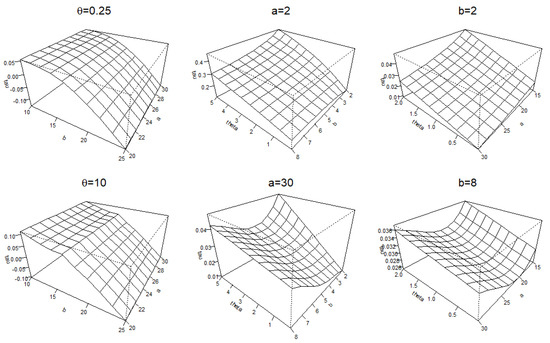
Consider the UL-Clayton copula in Example 8 and Kendall’s tau formula in Example 10. Figure 1 displays plots for the values of Kendall’s tau for various ranges of parameter values. They disclose that Kendall’s tau is not monotone in the parameter b when $a=30$ and in the parameter a when $b=8.$ They also confirm that the distorted copula is ordered by the parameter $\theta$ as the family of the Clayton copulas is ordered by the parameter $\theta .$

Figure 1. Kendall’s-tau surface plot for the UL-Clayton copula for various parameter values.

Example 14.

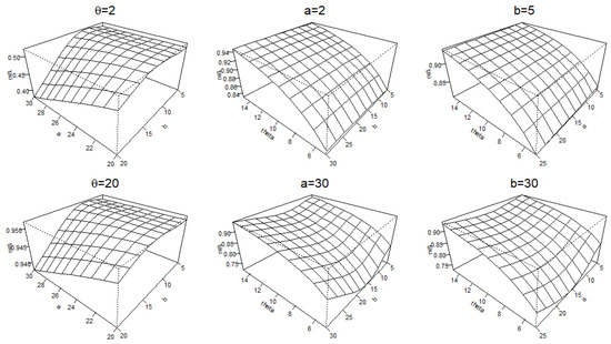
Consider the UL-Gumbel copula in Example 2 and Kendall’s tau formula in Example 11. As shown in Figure 2, e.g., Kendall’s tau is not monotone in b when$a=30$and in a when$b=30.$The concordance ordering in a or b can fail to hold. All plots show a monotone Kendall’s tau in$\theta .$

Figure 2. Kendall’s-tau surface plot for the UL-Gumbel copula for various parameter values.

Example 15.

Consider the UL-Frank copula in Example 4 and Kendall’s tau formula in Example 12. Figure 3 leads to the same conclusions observed from Figure 1 and Figure 2.

Figure 3. Kendall’s-tau surface plot for the UL-Frank copula for various parameter values.

7. Density Contour Plots and A Simulation Study

In this section, we feature some graphical and numerical results.

7.1. Density Contour Plots

Density contour plots can effectively illustrate the concordance and tail dependence behaviors between two variables. Figure 4 shows the contour plots for various bivariate probability densities, denoted by $h(x,y)$ in Section 1, using the UL distorted copulas with standard normal margins. The first row displays the contours constructed from the base copulas, the Clayton, Gumbel, and t-copulas; and the second and third rows the UL-distorted copulas, with $(a,b)=(1.5,2)$ and $(a,b)=(3,0.75),$ respectively. The parameter $\theta$ is chosen so that Kendall’s tau of the base copula is either 0.5 or $-0.5.$

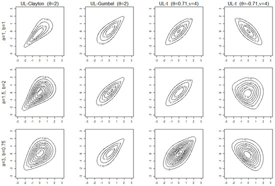
Figure 4. Density contour plots constructed from using the UL-distorted copulas with standard normal margins and parameter values $(a,b)=(1,1),(1.5,2),$ and $(3,0.75).$

For the t-copula, the degrees of freedom $\nu$ is 4 by default in R and the parameter $\theta$ is either 0.71 or $-0.71$. Note that t-copulas are reflective symmetric. Based on the plots in the first three columns, as shown in Theorem 1, when the parameter a increases the strength of lower tail dependence weakens or stays none, and the strength of upper tail dependence appears to remain the same for distorted copulas. The plots in the last column are constructed using a t-copula with a negative Kendall’s tau of $-0.5$ as the base copula. In this case, the definitions of tail dependence in Section 4 are not applicable; neither are Theorems 1 and 2.

7.2. A Simulation Study

We next conduct a simulation study, similar to those in Yang et al. (2011), to evaluate the flexibility of the UL-distorted copulas.

To generate bivariate data from the proposed copulas, we use the conditional distribution methods; see Devroye (1986) or Joe (2015). Let $C\left(v\right|u_1)=P(V\le v|U_1=u_1)=\partial C(u_1,v)/\partial u_1.$ The following algorithm is applied: (i) generate two independent random values $(u_1,v)$ from the uniform distribution on the unit interval and (ii) solve $C\left(u_2\right|u_1)=v$ for $u_2$. The desired pair is $(u_1,u_2)$

We simulated three bivariate data sets of 1000 observations from the Clayton, Gumbel, and t copulas with parameter values 2, 2, and $0.71$ ($\nu =4),$ receptively. The UL-distorted models were then fit to the three data sets. The parameters were estimated by the pseudo-likelihood estimation method described in Section 8 here. The P-P plots of empirical cdf and estimated cdf under each of the UL-distorted models are displayed in the first row of Figure 5. For the second row of P-P plots, three data sets of size 1000 were generated from the UL-Clayton, UL-Gumbel, and UL-t copulas with parameter $(\theta ,a,b)$ of $(2,1.5,3)$,$(2,1.5,3),$ and $(0.71,1.5,3),$ respectively. The degree of freedom for the t-copula is $4.$ We also fit widely used copulas such as the Clayton, BB1, Galambos, Gaussian, t, Gumbel, and Frank copulas to the second sets of simulated data.

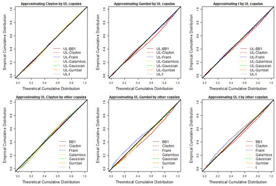
Figure 5. P-P plots of the empirical cumulative distribution and estimated cumulative distribution for various theoretical models. The first row displays the results from fitting data generated from the Clayton, Gumbel, and t copulas. The second row is from the UL-Clayton, UL-Gumbel, and UL-t-copulas.

The black curve is the one resulting from fitting the correct copula model. Reading the areas between the black and other curves, for example, the distribution for the data simulated from the Gumbel copula with upper tail dependence and no lower tail dependence appears to be approximated well by various UL-distorted copulas, except the UL-Clayton copula without upper tail dependence. However, the distribution for the data simulated from the UL-Gumbel copula appears to be approximated less well by non-distorted base copulas, except the Gumbel copula. One would expect the UL-distorted copulas to be more flexible due to extra parameter and more reliable in the sense that UL-distorted copula would tend to improve the fit.

8. Application

Here, we analyze CRSPday data to see the performance of the UL-distorted copulas. The data are readily available in “Ecdat” R package. It contains daily returns collected between 1989 and 1998 in the United States. We consider daily returns for IBM stock (IBM) and the historical value-weighted indexes (CRSP) by the Center for Research in Security Price. Based on the definition and research by the National Bureau of Economic Research (NBER) and Walsh (1993), the eight-month period between July 1990 and March 1991 is a recession in the NBER’s chronology. After the recession, the 1990s was a period of economic growth. We thus split the sample period into two sub-periods: the crisis period (July 1990 to March 1991) and the post-crisis period (April 1991 to December 1998). Splitting the sample allows us to explore the impact of a financial crisis and differences in the relations between the two variables, by using copula models.

Table 2 presents summary statistics in percentage of the two variables, including the standard deviation (SD), first quartile (Q1), and third quartile (Q3) for the crisis and post-crisis periods separately. Other than the maximum values for IBM, there are few differences between the crisis and post-crisis periods in summary statistics for the two variables.

Table 2. Summary statistics in percentage of IBM and CRSP during crisis and post-crisis periods.

Period	Variable	n	mean	min	Q1	Median	Q3	Max	SD
Crisis	IBM	209	0.00	$-9.97$	$-0.94$	0.00	0.94	6.07	1.55
	CRSP	209	0.04	$-3.15$	$-0.56$	0.00	0.66	3.31	1.00
Post-crisis	IBM	1962	0.09	$-10.74$	$-0.10$	0.00	1.05	12.94	1.86
	CRSP	1962	0.07	$-6.59$	$-0.26$	0.08	0.46	4.82	0.76

Scatter plots are displayed in Figure 6 to visualize possible data features, such as the joint behavior of extreme values between IBM and CRSP or between pseudo-IBM ($\widehat{v}$) and pseudo-CRSP ($\widehat{u}$), i.e, the empirical distributions of IBM and CRSP. The scatter plots indicate that there is a stronger agreement in IBM and CRSP for the crisis-period data than for the post-crisis data. Note that 0the sample Kendall’s taus for crisis and post-crisis periods are 0.55 and 0.30, respectively. From Figure 6a, there seems to be upper tail dependence and weak lower tail dependence in the crisis-period data. One might therefore choose copula models with upper tail dependence such as Galambos and Gumbel copulas in Table 3. For the post-crisis data, Figure 6b appears to have lower and upper tail dependence, in which case, t-copula and BB1 copulas might be appropriate.

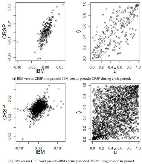
Figure 6. The scatter plots.

Table 3. MPLL, AIC, $\widehat{\tau },$ ${\widehat{\lambda }}_L,$ ${\widehat{\lambda }}_U,$ and parameter estimates (standard error in parentheses) for the base and UL distorted copulas during crisis period.

Family	MPLL	AIC	$\widehat{\mathit{\tau }}$	${\widehat{\mathit{\lambda }}}_{\mathit{L}}$	${\widehat{\mathit{\lambda }}}_{\mathit{U}}$	$\widehat{\mathit{\theta }}$	$\widehat{\mathit{a}}$	$\widehat{\mathit{b}}$
Clayton	63.8	$-125.5$	0.42	0.62	*	1.47(0.16)	–	–
Frank	78.9	$-155.8$	0.54	*	*	6.47(0.55)	–	–
Galambos	90.7	$-179.3$	0.54	*	0.62	1.47(0.17)	–	–
Gaussian	90.4	$-178.8$	0.55	*	*	0.77(0.03)	–	–
Gumbel	90.4	$-178.8$	0.39	*	0.47	1.64(0.05)	–	–
t	90.4	$-178.8$	0.56	0.28	0.28	0.77(0.03)	–	–
BB1	92.3	$-180.5$	0.55	0.27	0.57	0.27(0.15)	–	–
BB1	–	–	–	–	–	1.95(0.16)	–	–
UL-Clayton	63.8	$-121.5$	0.42	0.62	*	1.47(0.04)	1.00(0.28)	1.00(0.01)
UL-Frank	79.2	$-152.3$	0.54	*	*	6.72(0.71)	1.21(0.51)	1.15(0.19)
UL-Galambos	92.7	$-179.4$	0.55	*	0.56	1.21(0.18)	2.45(1.73)	6.01(0.88)
UL-Gaussian	92.1	$-178.2$	0.56	*	*	0.94(0.02)	19.13(0.54)	4.00(0.36)
UL-Gumbel	92.3	$-178.5$	0.55	*	0.57	1.92(0.19)	2.02(1.66)	4.00(0.80)
UL-t	92.1	$-178.2$	0.54	0.00	0.49	0.90(0.03)	9.00(0.48)	4.00(0.01)
UL-BB1	92.3	$-176.6$	0.55	0.09	0.57	0.35(0.40)	2.36(0.01)	2.98(0.50)
UL-BB1	–	–	–	–	–	1.92(0.21)	–	–

The asterisk notation (*) indicates that either the lower or the upper tail dependence coefficient has a value of 0.

The maximum pseudo-likelihood estimation (MPLE) introduced by Genest et al. (1995) is used to fit parameters of a copula model. Let $\left\{{(x_j,y_j)}_{j=1}^n\right\}$ be the set of observations. Define $\widehat{F}\left(x\right)={\sum }_{j=1}^{n}J(x_j\le x)/n$ and $\widehat{G}\left(y\right)={\sum }_{j=1}^{n}J(y_j\le y)/n,$ where $J(·)$ is the indicator function. The MPLE method first estimates the marginal distributions F and G using the empirical distributions $\widehat{F}$ and $\widehat{G},$ and then maximizes the pseudo-log-likelihood function given by

$$\begin{array}{c}\hfill L(\theta ,a,b)=\sum _{i=1}^{n}log{c}_T({\widehat{u}}_{1i},{\widehat{u}}_{2i};\theta ,a,b),\end{array}$$

(13)

where $c_T$ is the copula pdf and the pseudo-observations ${\widehat{u}}_{1i}=\widehat{F}\left(x_i\right)$ and ${\widehat{u}}_{2i}=\widehat{F}\left(y_i\right).$

In addition to the parameter estimates with their standard error in the parentheses, Table 3 containing results for the crisis-period data and Table 4 for the post-crisis data report the maximum pesudo-log-likelihood value (MPLL) in (13), AIC, $\widehat{\tau },$${\widehat{\lambda }}_L,$ and ${\widehat{\lambda }}_U.$ The asterisk notation (*) indicates that either the lower or the upper tail dependence coefficient has a value of 0. The parameter estimate computed for the base copula is used as the initial value when maximizing the UL-distorted copula models. The built-in R function optim() is employed to solve for the MPLE estimates.

Table 4. MPLL, AIC, $\widehat{\tau },$ ${\widehat{\lambda }}_L,$ ${\widehat{\lambda }}_U,$ and parameter estimates (standard error in parentheses) for the base and UL distorted copulas during post-crisis period.

Family	MPLL	AIC	$\widehat{\mathit{\tau }}$	${\widehat{\mathit{\lambda }}}_{\mathit{L}}$	${\widehat{\mathit{\lambda }}}_{\mathit{U}}$	$\widehat{\mathit{\theta }}$	$\widehat{\mathit{a}}$	$\widehat{\mathit{b}}$
Clayton	201.6	$-401.3$	0.24	0.35	*	0.66(0.04)	–	–
Frank	213.4	$-424.8$	0.31	*	*	3.00(0.15)	–	–
Galambos	200.3	$-399$	0.27	*	0.34	0.64(0.02)	–	–
Gaussian	231.1	$-460.3$	0.30	*	*	0.46(0.02)	–	–
Gumbel	203.3	$-404.7$	0.28	*	0.35	1.38(0.02)	–	–
t	240.5	$-477$	0.30	0.09	0.09	0.46(0.02)	–	–
BB1	240.6	$-477.3$	0.30	0.20	0.22	0.36(0.05)	–	–
BB1	–	–	–	–	–	1.20(0.03)	–	–
UL-Clayton	216.2	$-426.4$	0.33	0.51	*	1.04(0.18)	1.01(0.01)	3.98(0.09)
UL-Frank	223.8	$-441.6$	0.30	*	*	3.87(0.36)	2.15(0.43)	1.02(0.03)
UL-Galambos	239.8	$-473.7$	0.31	*	0.20	0.43(0.04)	2.04(0.59)	9.46(0.36)
UUL-Gaussian	238	$-470$	0.30	*	*	0.67(0.04)	4.72(1.26)	4.02(0.28)
UL-Gumbel	240.9	$-475.9$	0.30	*	0.21	1.19(0.03)	2.14(0.65)	10.75(0.44)
UL-t	242.1	$-478.1$	0.31	0.02	0.08	0.44(0.15)	1.57(1.88)	2.12(1.55)
UL-BB1	242.3	$-476.6$	0.30	0.12	0.18	0.28(0.08)	1.01(0.11)	1.88(0.74)
UL-BB1	–	–	–	–	–	1.16(0.03)	–	–

The asterisk notation (*) indicates that either the lower or the upper tail dependence coefficient has a value of 0.

Since the sample size for the crisis-period data is smaller, one would expect that the standard errors of parameter estimates for each model in Table 3 are larger than those in Table 4. Furthermore, the UL-distorted copula model is expected to perform better than its base copula model in terms of MPLL, due to the extra parameters.

In Table 3, not surprisingly, copula models with upper tail dependence perform well in terms of MPLL and AIC. The UL-distorted copula provides a better fit than its copula base in terms of the MPLL. AIC penalized a model for additional parameters. Two extra parameters are inoculated into the UL-distorted copula model. Partly due to the fact that a smaller sample size leads to a smaller likelihood value, the BB1 copula model is the winner in terms of AIC for fitting the crisis-period data.

For the post-crisis data, based on Table 4, the t-copula of the Elliptical class and the BB1 copula of the Archimedean class perform well. Just as for the crisis-period data, the Clayton and Frank copulas fit the data poorly in comparison with other copula models in the table. However, there is a sizable improvement in MPLL and AIC for the UL-Clayton and UL-Galambos copula models, which, in a way, reflects the simulation study results. The UL-distorted copula model outperforms its base copula in terms of MPLL. In terms of the AIC, the UL-BB1 copula model of four parameters offers no improvement over its base copula. The rest of the UL-distorted copula models of three parameters deliver a better fit than its base copula in terms of AIC. Among the selected models, the UL-distorted t-copula model is the best performer.

For the crisis data, the respective estimates for upper and lower tail dependence coefficients are 0.27 and 0.57, based on the BB1 copula model. For the post-crisis data, they are 0.01 and 0.08 based on the UL-t-copula. The estimated Kendall’s tau coefficients resulting from top performers are close to the sample Kendall’s tau coefficients of 0.55 and 0.30, for crisis and post-crisis data, respectively.

The UL-distortion induced model is expected to enhance the model fit in terms of MPLL. However, in terms of AIC, due to the penalization for extra parameters, the UL-distortion induced copula may not perform as well as its base copula.

The Cramer-von Mises goodness-of-fit statistic (CvM) is conducted to test the adequacy of copula models in Table 3. The CvM is calculated as the sum of square deviations between the empirical cdf and the estimated copula cdf. A bootstrap approach is used to approximate p-values; see Genest et al. (2009) for details. For the two sample sizes of 209 and 1962, we computed the bootstrapped p-value based on 1000 replications. Table 5 reports the results. For example, for post-crisis data, fitting the UL-t model results in a CvM value of 0.0354 with a p-value of almost 1 indicating the UL-t model is appropriate. While not all the base copulas chosen appear adequate, all the UL-distorted copula models provide an adequate fit based on Cramer-von Mises goodness-of-fit test.

Table 5. Cramer-von Mises test statistics in hundredths and p-values in parentheses for copulas in Table 3 and Table 4.

	Crisis Period			Post-Crisis Period
Model	Base	UL-Distorted		Base	UL-Distorted
BB1	1.25($\approx 1$)	1.21($\approx 1$)		1.78(0.37)	2.07($\approx 1$)
t	1.13(0.86)	1.76($\approx 1$)		2.26(0.21)	3.54($\approx 1$)
Gaussian	1.14(0.82)	1.14($\approx 1$)		1.14(0.85)	2.46($\approx 1$)
Gumbel	0.08(0.94)	1.17($\approx 1$)		8.70(0.00)	2.66($\approx 1$)
Galambos	0.06(0.96)	1.15($\approx 1$)		9.73(0.00)	5.04(0.94)
Frank	2.91(0.05)	3.12($\approx 1$)		6.96(0.05)	5.42(0.89)
Clayton	15.36(0.00)	15.51(0.44)		29.35(0.11)	23.25(0.18)

9. Concluding Remarks

This research proposes a mechanism to construct a distortion function and explores the properties of the family of copulas induced by the unit Lomax distortion. Explicit expressions for the UL-Clayton, UL-Gumbel, UL-independence, UL-Frank, UL-Galambos, and UL-BB1 copulas are given. In addition to the limiting cases in the parameters, the tail behaviors including the dependence coefficients and orders are studied for the UL distorted copulas. Kendall’s tau formulas for the UL-Clayton, UL-Gumbel, and UL-Frank copulas are derived and used to investigate the concordance ordering. The maximum pseudo-likelihood estimation is employed to fit the copula model. The Cramer-von Mises goodness-of-fit statistic is conducted to evaluate the adequacy of copula models. As expected, the UL-distorted copula outperforms its base copula.

The construction mechanism described in Section 2 utilizes a transformation of a nonnegative continuous random variable Y to a variable U, whose support is the unit interval. The paper considers the transformation of $U=1/(1+Y),$ where Y is a Lomax random variable. One possible candidate for Y is the Weibull random variable with cdf $1-e^{{(-bx)}^a},a,b>0$. However, upon further calculations, the resulting distortion is not admissible. There are undoubtedly other employable transformations and nonnegative random variables. An example is the transformation, $e^{-Y},$ of a Weibull random variable. We are currently examining this case. Distortion of multivariate copulas is more complicated and will be investigated further in a separate paper.

References

- Devroye, Luc. 1986. Non-Uniform Random Variate Generation. New York: Springer. [Google Scholar]
- Di Bernardino, Elena, and Didier Rulliere. 2013. On certain transformations of Archimedean copulas: Application to the non-parametric estimation of their generators. Dependence Modeling 1: 1–36. [Google Scholar] [CrossRef]
- Durante, Fabrizio, Rachele Foschi, and Peter Sarkoci. 2010. Distorted copulas: Constructions and tail dependence. Communications in Statistics. Theory and Methods 39: 2288–301. [Google Scholar] [CrossRef]
- Frees, Edward W., and Emiliano A. Valdez. 1998. Understanding relationships using copulas. North American Actuarial Journal 2: 1–25. [Google Scholar] [CrossRef]
- Genest, Christian, Bruno Remillard, and David Beaudoin. 2009. Goodness-of-fit tests for copulas: A review and a power study. Insurance: Mathematics and Economics 44: 199–213. [Google Scholar] [CrossRef]
- Genest, Christian, Kilani Ghoudi, and L. P. Rivest. 1995. A semiparametric estimation procedure of dependence parameters in multivariate families of distributions. Biometrika 82: 543–52. [Google Scholar] [CrossRef]
- Gudendorf, Gordon, and Johan Segers. 2010. Extreme-value copulas. Copula Theory and Its Applications Lecture Notes in Statistics, 127–45. [Google Scholar]
- Joe, Harry, and Taizhong Hu. 1996. Multivariate distributions from mixtures of max-infinitely divisible distributions. Journal of Multivariate Analysis 57: 240–65. [Google Scholar] [CrossRef]
- Joe, Harry. 2015. Dependence Modeling with Copulas. Boca Raton: CRC Press. [Google Scholar]
- Lin, Feng, Liang Peng, Jiehua Xie, and Jingping Yang. 2018. Stochastic distortion and its transformed copula. Insurance: Mathematics and Economics 79: 148–66. [Google Scholar] [CrossRef]
- Nelsen, Roger B. 1997. Dependence and order in families of Archimedean copulas. Journal of Multivariate Analysis 60: 111–22. [Google Scholar] [CrossRef]
- Nelsen, Roger B. 2006. An Introduction to Copulas. New York: Springer. [Google Scholar]
- Nguyen, Thu Thuy, Van Chien Nguyen, and Trong Nguyen Tran. 2020. Oil price shocks against stock return of oil-and gas-related firms in the economic depression: A new evidence from a copula approach. Cogent Economics & Finance 8: 1799908. [Google Scholar]
- Samanthi, Ranadeera G. M., and Jungsywan Sepanski. 2019. A bivariate extension of the beta generated distribution derived from copulas. Communications in Statistics—Theory and Methods 48: 1043–59. [Google Scholar] [CrossRef]
- Sepanski, Jungsywan. H. 2020. A note on distortion effects on the strength of bivariate copula tail dependence. Statistics & Probability Letters 166: 108–894. [Google Scholar]
- Sklar, Abe. 1959. Fonctions de repartition a n dimensions et leurs marges. Publications de l’Institut Statistique de l’Universite de Paris 8: 229–31. [Google Scholar]
- Valdez, Emiliano A., and Yugu Xiao. 2011. On the distortion of a copula and its margins. Scandinavian Actuarial Journal, 292–317. [Google Scholar] [CrossRef]
- Walsh, Carl E. 1993. What caused the 1990-1991 recession? Economic Review, Federal Reserve Bank of San Francisco 2: 33–48. [Google Scholar]
- Yang, Xipei, Edward W. Frees, and Zhengjun Zhang. 2011. A generalized beta copula with applications in modeling multivariate long-tailed data. Insurance: Mathematics and Economics 49: 265–84. [Google Scholar] [CrossRef]
Publisher‘s Note: MDPI stays neutral with regard to jurisdictional claims in published maps and institutional affiliations. |
© 2020 by the authors. Licensee MDPI, Basel, Switzerland. This article is an open access article distributed under the terms and conditions of the Creative Commons Attribution (CC BY) license (http://creativecommons.org/licenses/by/4.0/).