Abstract
The present study aims at modelling market risk for four commodities, namely West Texas Intermediate (WTI) crude oil, natural gas, gold and corn for the period 2007–2017. To this purpose, we use Extreme Value Theory (EVT) together with a set of Conditional Auto-Regressive Logit (CARL) models to predict risk measures for the futures return series of the considered commodities. In particular, the Peaks-Over-Threshold (POT) method has been combined with the Indicator and Absolute Value CARL models in order to predict the probability of tail events and the Value-at-Risk and the Expected Shortfall risk measures for the selected commodities. Backtesting procedures indicate that generally CARL models augmented with specific implied volatility outperform the benchmark model and thus they represent a valuable tool to anticipate and manage risks in the markets.
1. Introduction
Energy, metal and agricultural commodities are very relevant in everyday life for a number of reasons. To start with, they play a crucial role in the global economy, since changes in their prices (and their volatility) have an impact on consumers, producers and the general economic activity. This is particularly true for oil, given that its rising prices generate not only effects on the demand and supply side of the economy, but also on financial markets. For instance, Sadorsky (1999) showed that shocks to oil prices tend to depress real stock returns. More recently, Algieri and Leccadito (2017) documented contagion effects from commodity markets to the rest of the economy. Specifically, they demonstrated that adverse shocks hitting one or more commodity markets tend to spread to the entire economic system as a consequence of the financialisation and integration processes of commodity markets.
Similarly, the intensified price interlinkages between energy and agricultural prices have raised concerns about deeper volatility connections and likely adverse effects on economic actors. More volatile agricultural prices can lead to sub-optimal productions, make poor consumers in countries dependent on grains more vulnerable to price swings, with the consequent increase in social and political tensions (Mensi et al. 2017; Tadesse et al. 2014).
Another reason for the importance of energy and non-energy commodities stems from their increasing role in portfolio strategies over the last two decades (Bhardwaj et al. 2016; Tang and Xiong 2012). Indeed, commodities are perceived as an alternative instrument to equities and fixed income securities, due to their low correlation with those two asset classes, and, as such, offer an interesting diversification opportunity and, in some cases, represent a ‘safe haven’. For instance, gold and oil have emerged as an important hedging tool to diversify market risk and precious metals have been widely used in risk management strategies. However, the stronger price volatility interlinkages across commodities could weaken the diversification benefits of holding commodities in a portfolio (Kumar et al. 2019).
For the aforementioned reasons, it is crucial to identify appropriate statistical models to quantify and measure the risks associated with commodities. Over the recent years, Value-at-Risk (VaR) and Expected Shortfall (ES) have been adopted in the literature as risk measures especially for the examination of the risks linked to equities, interest rates and foreign exchanges. Commodity price risk evaluation has received less attention compared to other asset classes.
Most of the analyses on commodities have scrutinised the linkages and the dependence structure of different asset classes. The studies on co-movements and risk dependences across commodities adopt several techniques including cointegration and correlation measures (de Nicola et al. 2016; Nazlioglu and Soytas 2012), SVAR models (Fernandez-Perez et al. 2016), non-linear ARDL models (Rehman et al. 2019), GARCH–family models (Algieri 2014a; Kang et al. 2017; Mensi et al. 2014), network models (Antonakakis et al. 2018; Ji et al. 2018), wavelet analysis (Mensi et al. 2017), pair vine copula models (Kumar et al. 2019) and conditional value-at-risk measures (Tiwari et al. 2020; Bouri et al. 2018; Shahzad et al. 2018).
In our study, we do not examine tail dependence across commodity pairs, but assess commodity market risk for single commodity over a short-term time horizon by considering the history of commodity returns and enclosing the typical features of their time series, such as fat tails. In this respect, we focus on purely statistical models to describe the evolution of commodity returns without relying on economic models that aim to forecast commodity prices considering supply and demand imbalances (Giot and Laurent 2003). Our approach allows the characterisation of risks for single commodity useful to disentangle specific commodity risk patterns.
More in detail, to capture the behaviour of the tails for the commodity return distributions, we adopt the Extreme Value Theory (EVT) and, similar to Taylor and Yu (2016), combine it with models that assume tail probabilities evolving over time as an auto-regressive process (the Conditional Auto-Regressive Logit models (CARL) models). According to the Extreme Value Theory, the tail of a distribution can be, at least approximately, described by the so-called Generalised Pareto Distribution (GPD) (Pickands 1975). We follow the Peaks-Over-Threshold (POT) method and fit the GPD to losses larger than a given threshold. The POT method allows us to identify the magnitude of threshold exceedances. Then, we consider a time-varying scale parameter of the GPD which follows an auto-regressive process in order to obtain a Time Varying POT (TVPOT). Finally, tail probabilities entering the TVPOT method are made time varying by means of CARL models. The latter methods explain tail probabilities (constructed as twice the logit of probabilities) as a function of past extreme events, past returns and lagged values of some explanatory variables. CARL family models were introduced by Taylor and Yu (2016) as an improvement of older models including those by Rydberg and Shephard (2003) and Anatolyev and Gospodinov (2010). In the context of energy markets, CARL models have been shown to have a a better performance in forecasting tail probabilities than alternative models such as Historical Simulation, GARCH and Quantile-Augmented Volatility models (Algieri and Leccadito 2019).
In our analysis, we use the TVPOT methodology to forecast Value-at-Risk (VaR) and Expected Shortfall (ES) for four commodities of different type, namely WTI crude oil, natural gas, gold and corn, and backtest the latter measure using recently proposed testing procedures.
Despite not being coherent (a risk measure is said to be coherent if it satisfies a number of desirable mathematical properties (see Artzner et al. 1999)), Value-at-Risk, defined as a quantile of the profit and loss distribution, is the most popular risk measure among practitioners and regulators due to its simplicity (for instance, the capital requirement prescribed by Solvency II is the 0.5% VaR of the annual loss distribution). VaR, however, is insensitive to the severity of tail losses, by its definition of a quantile. Recent regulatory accords have thus shifted emphasis to Expected Shortfall, which is defined as the expected value of the profit and loss given that VaR has been exceeded. Basel III indeed prescribes 10-day 2.5%-ES as the risk measure on which capital requirements are to be based. Furthermore, ES has been proven to be a coherent risk measure (Acerbi and Tasche 2002).
Thus, in our study, we assess the accuracy of ES predictions for the proposed models using the multinomial tests introduced by Kratz et al. (2018). The latter category of testing procedures, while designed to backtest ES, are based on the idea that ES is successfully backtested if a number of VaRs at properly chosen coverage probabilities has been simultaneously successfully backtested and, hence, they only require the sequences of VaR violations (the so-called hit sequences) at the different coverage thresholds.
2. Methodology
Financial risks are generally linked to possible losses in financial markets stemming from interest rate changes, foreign currency fluctuations, equity and commodity price variations. Specifically, commodity market risk is the financial risk connected to sharp and excessive price fluctuations (Algieri 2014b; Giot and Laurent 2003). Predicting market risks and the time varying probability that a given financial asset return would overpass a specific threshold is very important for anticipating unstable and agitated times in the markets, managing risks and tuning investment strategies. In the following sections, we try to forecast tail probabilities associated to extreme return downturns of energy and non-energy commodities and predict VaR and ES risk measures by implementing first the POT methodology, then the Conditional Auto-Regressive Logit (CARL) models and finally combining the two methods.
2.1. POT Methods
The Peak-Over-Threshold method (POT-method) is a tool to model extreme values originally introduced by Smith (1989) and Davison and Smith (1990). The basic idea of this method is to consider a threshold to separate the values considered extreme from the rest of the data and build up a model for the extreme values by modelling the tails of the values exceeding the considered threshold. For some sufficiently large thresholds, the distribution of the values exceeding the cut-off approximates to a General Pareto Distribution with some ‘shape’ and ‘scale’ parameter.
Denote by the return associated to a given futures commodity. To describe Peaks-Over-Threshold methods, we follow the standard practice to work with losses (i.e., the negative of returns) rather than returns. Let denote the loss on day t for being long on the futures. The assumption underlying the POT method is that, when the loss exceeds a high threshold Q, the exceedance , follows a GPD described by the following cumulative distribution function (CDF):
where is the scale parameter and the shape parameter of the distribution. A positive shape parameter (, Frechet type) refers to a heavy tail distribution, a negative shape parameter (, Weibull type) corresponds to a bounded tail and a zero-value shape parameter (, Gumbel type) refers to a light tail distribution. In the above model, the following property of the conditional probabilities holds true for (see for instance McNeil et al. 2005, p. 283):
Using Equation (2) with is defined implicitly from
and typical values for are or ) and then using Equation (1), gives the following expression for value-at-risk with level :
The resulting expression for the corresponding is easily found to be:
Following Taylor and Yu (2016), we assume that the scale parameter of the GPD evolves according to the following auto-regressive model:
where the index j refers to a period with an exceedance, i.e., . To simplify the estimation, variance targeting is used, so that , where is estimated as the product of the variance of the exceedances and . The choice appears reasonable because for a random variable with CDF (1) the variance equals . Denote by the vector of parameters to be estimated, then, the Maximum Likelihood Estimation (MLE) can be used. In particular, assuming that exceedances are conditional on the scale parameter, independent and identically distributed with the CDF in Equation (1), the log-likelihood function reads:
where indicates the number of exceedances in the sample. It should be noted that Equation (6) is maximised under the constraints (needed to ensure positivity of ), and , in order to ensure stationarity and positivity of for all j.
2.2. CARL Models
In this section, we indicate with the conditional probability that falls below a fixed threshold Q, , where is the available information up to time t.
Following Taylor and Yu (2016), we model the dynamics (the inverse transformation yields , so that is forced to vary between 0 and when the threshold Q takes on negative values. is the indicator function, taking on value 1 if A is true and 0 otherwise) of and consider several Conditional Auto-Regressive Logit specifications.
The first specification for , called the CARL Indicator (CARL-Ind) model, is given by:
where is a binary–valued stochastic process that takes the value 1 if the lagged returns (one-period) are below the Q cut-off, and 0 otherwise. enables the tail probability to vary according to whether or not a return drop was registered in the previous period. The term gives the auto-regressive structure to the model and represents persistence.
The second considered specification is the CARL Absolute (CARL-Abs) model, formulated as:
While in CARL-Ind models the explanatory variable (besides the lagged term ) is binary, in CARL Absolute models the exceedance probability is explained by the commodity absolute return at time . The term appearing in Equation (8) can be considered a proxy for return volatility.
Many alternative models to Equations (7) and (8) are available (see Algieri and Leccadito 2019; Taylor and Yu 2016), and can be obtained, for instance, by adding to the above equations terms capturing asymmetries.
The models in Equations (7) and (8) can be augmented by adding one or more explanatory variables to the logit of the exceedance probability. The augmented specifications are denoted by CARL-X models. Thereby, CARL Absolute model and CARL Indicator model with explanatory variables (CARL-Abs-X and CARL-Ind-X ) can be described by the following equations respectively:
where is a vector of exogenous variables that could explain and is the corresponding vector of parameters.
Both models and their augmented versions can be estimated using the Maximum Likelihood Estimation method (MLE). The simplest approach is to assume that is conditionally Bernoulli distributed. In this case, the log-likelihood function is equal to
where T is the number of observations and is the parameter vector. A drawback of the approach based on the Bernoulli distribution is that it does not take into account how far is from Q when the indicator appearing in Equation (11) equals one. An approach based on the asymmetric Laplace (AL) distribution addresses this issue. Indeed, Taylor and Yu (2016) proposed using a quasi-maximum likelihood estimation based on the AL distribution. Using the function , the resulting penalised log-likelihood function is given by:
where is the returns mean. Details on the derivation of the above log-likelihood function can be found in Section 3.2 of Taylor and Yu (2016).
3. Empirical Application
Following Taylor and Yu (2016), we combine the methods presented in Section 2.1 and Section 2.2 to predict VaR and ES risk measures. In particular, given an estimation window of length T, we consider out-of-sample VaR forecasts for time using Equation (3) with the estimated parameters based on the window and the forecast for the tail probability The latter is obtained using the estimated parameter vector , again based on the window of T observations. The accuracy of the prediction is established via the recent tests of Kratz et al. (2018).
3.1. Data Description
To model tail risks and predict the time varying probability that commodity returns would exceed a given threshold, we compute daily log returns for WTI crude oil, gold, natural gas and corn by considering their first generic futures contracts extracted from Bloomberg (tickers CL1, GC1, HO1, and C1, respectively). The investigation covers the period 2 December 2003 to 27 October 2017, for a total of 3500 daily observations. Time-series plots for futures prices of the four commodities are given in Figure 1. It is interesting to notice that, while corn and energy commodity prices registered severe falls during the global financial crisis of 2008, gold was the only commodity to act in a counter-cyclical manner. This behaviour testifies the hedging feature of this precious metal.
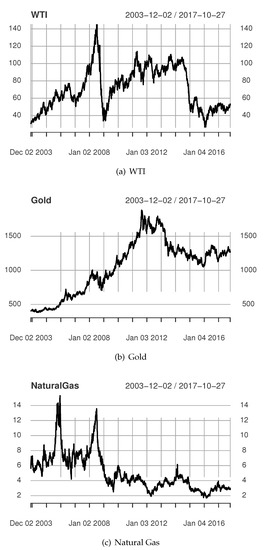
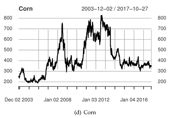
Figure 1.
Time-series plots for futures prices of the four commodities.
Daily returns for each commodity i are computed as log differences in futures price ():
Table 1 reports the descriptive statistics for daily futures returns. From the table, it is clear that the commodity with highest volatility is natural gas. Indeed, the standard deviations suggest that this energy commodity records the highest dispersion around the mean in comparison to other commodities, while gold shows the lowest volatility, thus confirming its characteristic of safe-haven. In addition, the average returns are higher for gold and WTI crude oil, while are negative for natural gas. The largest daily loss on commodity futures is 26.86 per cent for corn, followed by natural gas, crude oil and gold.

Table 1.
Summary Descriptive Statistics of Commodity Futures Returns.
Natural gas displays the highest positive skewness, which implies frequent small losses and a few extreme gains compared to the other commodities. Gold and corn returns are negatively skewed, meaning frequent small gains and a few extreme losses. All series are not distributed as a bell-shaped Gaussian, since the Jarque–Bera test displays a p-values of zero and there is an excess kurtosis especially for corn. The results of the Augmented Dickey–Fuller unit root test suggest that all return are stationary given that the null hypothesis of unit root is always rejected.
Table 2 presents the correlation coefficients of the four commodity returns. It can be noticed that the correlation across commodities is always positive and it never overcomes 25 per cent. This means that there are not significant relationships among commodities, and they can be used to diversify investment portfolios.
Table 2.
Correlation Matrix of Commodity Returns.
In our analysis, commodity log returns represent our dependent variable and commodity implied volatility is used as explanatory variable in some variants of the adopted CARL models.
In particular, the implied volatility is calculated from prices of at-the-money (call) options expiring at least twenty business days from the observation date. This metrics is considered a forward-looking indicator for future return volatility. We consider the inverse of the implied volatility in line with Algieri and Leccadito (2019).
To assess how accurately our predictive model performs, we build out-of sample predictions. Specifically, we recursively estimate the parameters using a rolling window of observations to obtain a new one-period-ahead forecast. We use 2500 rolling windows each of length 1000. This implies that the first prediction is made for the end of November 2007.
Figure 2 plots the (negative of the) returns over an evaluation period of about 10 years. We select the threshold Q to the 85% unconditional quantile of the losses . This choice guarantees that the exceedance probability is larger than for each in-sample period with an exceedance. In particular, Figure 2 shows that the estimated measures of risk probability tend to move in the same fashion of returns. The VaR measures lay always below the ES measures by construction.
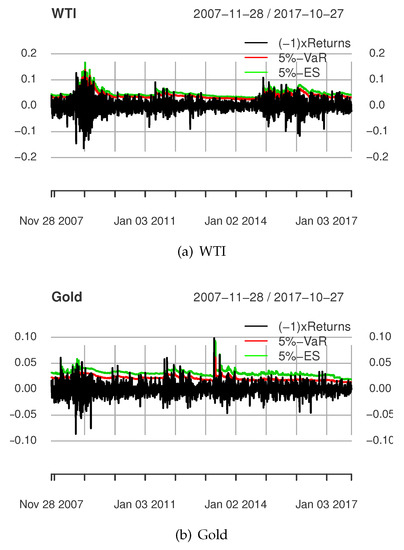
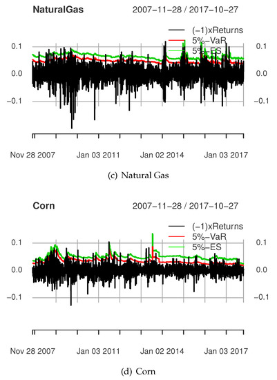
Figure 2.
Evolution over time of 5%-VaR and 5%-ES calculated using the ABS model combined with the POT method.
3.2. ES Testing Procedures
To evaluate the accuracy of the considered models to predict ES, we implement the multinomial test of Kratz et al. (2018). The testing procedure is based on a formula that approximates the -ES as the mean of a number of quantiles associated to equally spaced probability levels, with the largest one equal to . Explicitly:
The idea is therefore that is successfully backtested if the VaRs with levels with are deemed reliable since they have been simultaneously backtested. Assume K critical thresholds so that and ; we have, by convention, , , . Violations are defined for via the exception indicator series ( denotes the indicator function taking on value 1 if A is true and 0 otherwise.) Let be the total number of VaR violations in period at the different thresholds. Denote by the probability of falling in between the VaR associated to and , with . Assuming a number of observations equal to T, the number of observations falling between and are defined as . If both the unconditional coverage hypothesis—i.e., that , , for all t—and the independence hypothesis—i.e., is independent of for —hold, then the random vector follows the multinomial distribution, . Kratz et al. (2018) proposed several procedures to test the above hypotheses. The Pearson type of test is defined as:
and under the null it has a chi-square distribution with K degrees of freedom. A correction to the above test is given by the Nass test defined as where The null distribution of the Nass test statistic is chi-square with degrees of freedom. Finally, Kratz et al. (2018) considered the Likelihood-Ratio Test (LRT) defined as:
which, under the null, is chi-squared distributed with K degrees of freedom.
Results of the above testing procedures for and are reported in Table 3 and Table 4, respectively. In detail, the tables show the estimated p-values for the Indicator and Absolute CARL models and their augmented version with the implied volatility used as explanatory variable. For a comparison with alternative models, Table 3 and Table 4 further report the p-values obtained using a Normal GARCH (1,1), the Historical Simulation (HS), the Filtered Historical Simulation (FHS) methods (the FHS method we consider involves modeling the variance) and the Quantile-Augmented Volatility (QAV) model (see Han 2016 and Appendix A of Algieri and Leccadito 2019 for details on QAV models) proposed by Han (2016).
Table 3.
p-values for the Testing Procedures for -ES based on . The threshold Q is equal to the 85% unconditional quantile of the losses .
Table 4.
p-values for the Testing Procedures for -ES based on . The threshold Q is equal to the 85% unconditional quantile of the losses .
According to all the procedures, the best model to forecast 5%-ES is the augmented CARL-Abs-X model for crude oil, the augmented CARL-Ind-X models for gold and natural gas and the simple CARL-Ind model for corn. Conventional econometric models based on GARCH-methods are less capable to model and predict extreme commodity returns showing relevant time-varying volatility. This finding is consistent with most of the previous conclusions that commodity markets tend to suffer from extreme shocks (Ji and Fan 2012; Pindyck and Rotemberg 1990), and that there is some heterogeneity between oil and gas markets that indicates that the two commodities are not perfect substitutes (Ji et al. 2018) and, therefore, different prediction models can be necessary to forecast their tail risks. In addition, the results confirm that implied volatility linked to products can be considered a important variable to improve forecasting models and thereby facilitate risk management (Algieri and Leccadito 2017; Mensi et al. 2017).
The threshold Q plays a crucial role in the TVPOT-CARL models (and EVT in general). Indeed, there is a trade-off in the choice of Q. If the threshold is too large, then only few observations are left in the tail and it becomes difficult to accurately estimate the parameters of the GPD. However, choosing Q too small on the one hand increases the number of exceedances and, hence, the number of observations used when estimating the GPD parameters, but on the other hand it implies that the focus is no longer (only) on the tail of the distribution and the GPD may not be used to describe exceedances. As a robustness check, we consider alternative values for Q. In particular, Table 5 and Table 6 give the results of the testing procedures to assess the accuracy of -ES predicted using the TVPOT-CARL models when Q is equal to the 83% and 87% unconditional quantile of the losses, respectively. Overall, the findings presented in Table 5 and Table 6 confirm the outcomes registered for the 85% quantile.
Table 5.
p-values for the Testing Procedures for -ES based on and . The threshold Q is equal to the 83% unconditional quantile of the losses .
Table 6.
p-values for the Testing Procedures for -ES based on and . The threshold Q is equal to the 87% unconditional quantile of the losses .
In brief, the adoption of CARL with the POT methods could be considered an important technical tool to regularly monitor and minimise the market exposure to price risks and, at the same time, build optimal strategies that maximise investors’ profitability given a certain acceptable amount of risk.
4. Conclusions
Commodity markets are often characterised by high uncertainty and pronounced price volatility. These dynamics and the consequent hazy market conditions make necessary an examination of the most appropriate methodologies and tools to predict extreme price risks. To this purpose, we considered a novel class of models to measure and forecast tail events for WTI crude oil, natural gas, gold and corn over the years 2007–2017.
In particular, we used the Time Varying Peaks-Over-Threshold (TVPOT) method combined with a set of Conditional Auto-Regressive Logit (CARL) models and compared them with alternative benchmark models. After predicting the Value-at-Risk and Expected Shortfall risk measures specific to each commodity, we backtested 5%-ES to establish which model is accurate in measuring market risk.
We found that conventional econometric models based on GARCH, HS, FHS and QAV methods are less able to characterise the dynamics of commodity returns and forecast tail events and, hence, Expected Shortfall. Conversely, the TVPOT methodology in combination with CARL models and their augmented versions, which include time-varying implied volatility, generally allows more accurate risk predictions. The results further highlight that different commodities appear to work better with different variants of CARL-models. In particular, better forecasts are obtained using the augmented CARL-Abs-X model for crude oil, the augmented CARL-Ind-X models for gold and natural gas and the simple CARL-Ind model for corn. Some heterogeneity between oil and gas markets would confirm that the two commodities are not perfect substitutes and, therefore, different prediction models are necessary to forecast their tail risks.
The adoption of CARL within the POT framework could be useful for portfolio managers, risk arbitrageurs and traders who closely monitor commodity market trends and need to have a better knowledge on possible changes in prices for their investments and risk management decisions. At the same time, CARL and POT models would be useful to policy makers to predict in advance risks and therefore protect the poor from the severe impact of high food and energy prices. This is because the poorest segments of society are more exposed to increases in commodity prices given the large share especially of food and in their overall consumption basket.
Author Contributions
All authors contributed equally to the paper. All authors have read and agreed to the published version of the manuscript.
Funding
This research received no external funding.
Acknowledgments
The authors are grateful to the Editor, Mogens Steffensen and three anonymous reviewers for their insightful comments. The authors wish to thank Joachim von Braun and Antonio Aquino for their valuable suggestions and comments. The first author gratefully acknowledges financial support from the Federal Ministry for Economic Cooperation and Development, BMZ under the Center for Development Research (ZEF) (Scientific Research Program on ‘Volatility in commodity markets, trade policy and the poor’).
Conflicts of Interest
The authors declare no conflict of interest.
References
- Acerbi, Carlo, and Dirk Tasche. 2002. On the coherence of expected shortfall. Journal of Banking & Finance 26: 1487–503. [Google Scholar]
- Algieri, Bernardina. 2014a. The influence of biofuels, economic and financial factors on daily returns of commodity futures prices. Energy Policy 69: 227–47. [Google Scholar] [CrossRef]
- Algieri, Bernardina. 2014b. A roller coaster ride: an empirical investigation of the main drivers of the international wheat price. Agricultural Economics 45: 459–75. [Google Scholar] [CrossRef]
- Algieri, Bernardina, and Arturo Leccadito. 2017. Assessing contagion risk from energy and non-energy commodity markets. Energy Economics 62: 312–22. [Google Scholar] [CrossRef]
- Algieri, Bernardina, and Arturo Leccadito. 2019. Ask CARL: Forecasting tail probabilities for energy commodities. Energy Economics 84: 104497. [Google Scholar] [CrossRef]
- Anatolyev, Stanislav, and Nikolay Gospodinov. 2010. Modeling financial return dynamics via decomposition. Journal of Business & Economic Statistics 28: 232–45. [Google Scholar]
- Antonakakis, Nikolaos, Tsangyao Chang, Juncal Cunado, and Rangan Gupta. 2018. The relationship between commodity markets and commodity mutual funds: A wavelet-based analysis. Finance Research Letters 24: 1–9. [Google Scholar] [CrossRef]
- Artzner, Philippe, Freddy Delbaen, Jean-Marc Eber, and David Heath. 1999. Coherent measures of risk. Mathematical Finance 9: 203–28. [Google Scholar] [CrossRef]
- Bhardwaj, Geetesh, Gary B. Gorton, and Kevin G. Rouwenhorst. 2016. Investor interestand the returns tocommodity investing. The Journal of Portfolio Management 42: 44–55. [Google Scholar] [CrossRef]
- Bouri, Elie, Rangan Gupta, Amine Lahiani, and Muhammad Shahbaz. 2018. Testing for asymmetric nonlinear short- and long-run relationships between bitcoin, aggregate commodity and gold prices. Resources Policy 57: 224–35. [Google Scholar] [CrossRef]
- Davison, A. C., and R. L. Smith. 1990. Models for exceedances over high thresholds. Journal of the Royal Statistical Society. Series B (Methodological) 52: 393–442. [Google Scholar] [CrossRef]
- de Nicola, Francesca, Pierangelo De Pace, and Manuel A. Hernandez. 2016. Co-movement of major energy, agricultural, and food commodity price returns: A time-series assessment. Energy Economics 57: 28–41. [Google Scholar] [CrossRef]
- Fernandez-Perez, Adrian, Bart Frijns, and Alireza Tourani-Rad. 2016. Contemporaneous interactions among fuel, biofuel and agricultural commodities. Energy Economics 58: 1–10. [Google Scholar] [CrossRef]
- Giot, Pierre, and Sebastien Laurent. 2003. Market risk in commodity markets: A VaR approach. Energy Economics 25: 435–57. [Google Scholar] [CrossRef]
- Han, Heejoon. 2016. Quantile Dependence between Stock Markets and its Application in Volatility Forecasting. arXiv arXiv:1608.07193. [Google Scholar]
- Ji, Qiang, and Ying Fan. 2012. How does oil price volatility affect non-energy commodity markets? Special issue on Thermal Energy Management in the Process Industries. Applied Energy 89: 273–80. [Google Scholar] [CrossRef]
- Ji, Qiang, Elie Bouri, David Roubaud, and Syed Jawad Hussain Shahzad. 2018. Risk spillover between energy and agricultural commodity markets: A dependence-switching covar-copula model. Energy Economics 75: 14–27. [Google Scholar] [CrossRef]
- Kang, Sang Hoon, Ron McIver, and Seong-Min Yoon. 2017. Dynamic spillover effects among crude oil, precious metal, and agricultural commodity futures markets. Energy Economics 62: 19–32. [Google Scholar] [CrossRef]
- Kratz, Marie, Yen H. Lok, and Alexander J. McNeil. 2018. Multinomial VaR backtests: A simple implicit approach to backtesting expected shortfall. Journal of Banking & Finance 88: 393–407. [Google Scholar]
- Kumar, Satish, Aviral Kumar Tiwari, I. D. Raheem, and Qiang Ji. 2019. Dependence risk analysis in energy, agricultural and precious metals commodities: a pair vine copula approach. Applied Economics, 1–18. [Google Scholar] [CrossRef]
- McNeil, Alexander J., Rudiger Frey, and Paul Embrechts. 2005. Quantitative Risk Management: Concepts, Techniques And Tools. Princeton Series in Finance; Princeton: Princeton University Press. [Google Scholar]
- Mensi, Walid, Shawkat Hammoudeh, Duc Khuong Nguyen, and Seong-Min Yoon. 2014. Dynamic spillovers among major energy and cereal commodity prices. Energy Economics 43: 225–43. [Google Scholar] [CrossRef]
- Mensi, Walid, Aviral Tiwari, Elie Bouri, David Roubaud, and Khamis H. Al-Yahyaee. 2017. The dependence structure across oil, wheat, and corn: A wavelet-based copula approach using implied volatility indexes. Energy Economics 66: 122–39. [Google Scholar] [CrossRef]
- Nazlioglu, Saban, and Ugur Soytas. 2012. Oil price, agricultural commodity prices, and the dollar: A panel cointegration and causality analysis. Energy Economics 34: 1098–104. [Google Scholar] [CrossRef]
- Pickands, James, III. 1975. Statistical inference using extreme order statistics. Annals of Statistics 3: 119–31. [Google Scholar] [CrossRef]
- Pindyck, Robert S., and Julio J. Rotemberg. 1990. The excess co-movement of commodity prices. The Economic Journal 100: 1173–89. [Google Scholar] [CrossRef]
- Rehman, Mobeen Ur, Elie Bouri, Veysel Eraslan, and Satish Kumar. 2019. Energy and non-energy commodities: An asymmetric approach towards portfolio diversification in the commodity market. Resources Policy 63: 1–19. [Google Scholar] [CrossRef]
- Rydberg, Tina Hviid, and Neil Shephard. 2003. Dynamics of trade-by-trade price movements: Decomposition and models. Journal of Financial Econometrics 1: 2–25. [Google Scholar] [CrossRef]
- Sadorsky, Perry. 1999. Oil price shocks and stock market activity. Energy Economics 21: 449–69. [Google Scholar] [CrossRef]
- Shahzad, Jawad, Jose Arreola Hernandez, Khamis Al-Yahyaee, and Rania Jammazi. 2018. Asymmetric risk spillovers between oil and agricultural commodities. Energy Policy 118: 182–98. [Google Scholar] [CrossRef]
- Smith, Richard L. 1989. Extreme value analysis of environmental time series: An application to trend detection in ground-level ozone. Statistical Science 4: 367–77. [Google Scholar] [CrossRef]
- Tadesse, Getaw, Bernardina Algieri, Matthias Kalkuhl, and Joachim von Braun. 2014. Drivers and triggers of international food price spikes and volatility. Food Policy 47: 117–28. [Google Scholar] [CrossRef]
- Tang, Ke, and Wei Xiong. 2012. Index investment and the financialization of commodities. Financial Analysts Journal 68: 54–74. [Google Scholar] [CrossRef]
- Taylor, James W., and Keming Yu. 2016. Using auto-regressive logit models to forecast the exceedance probability for financial risk management. Journal of the Royal Statistical Society: Series A (Statistics in Society) 179: 1069–92. [Google Scholar] [CrossRef]
- Tiwari, Aviral Kumar, Nader Trabelsi, Faisal Alqahtani, and Ibrahim D. Raheem. 2020. Systemic risk spillovers between crude oil and stock index returns of g7 economies: Conditional value-at-risk and marginal expected shortfall approaches. Energy Economics 86: 104646. [Google Scholar] [CrossRef]
© 2020 by the authors. Licensee MDPI, Basel, Switzerland. This article is an open access article distributed under the terms and conditions of the Creative Commons Attribution (CC BY) license (http://creativecommons.org/licenses/by/4.0/).