Estimation of Star-Shaped Distributions

Abstract

Scatter plots of multivariate data sets motivate modeling of star-shaped distributions beyond elliptically contoured ones. We study properties of estimators for the density generator function, the star-generalized radius distribution and the density in a star-shaped distribution model. For the generator function and the star-generalized radius density, we consider a non-parametric kernel-type estimator. This estimator is combined with a parametric estimator for the contours which are assumed to follow a parametric model. Therefore, the semiparametric procedure features the flexibility of nonparametric estimators and the simple estimation and interpretation of parametric estimators. Alternatively, we consider pure parametric estimators for the density. For the semiparametric density estimator, we prove rates of uniform, almost sure convergence which coincide with the corresponding rates of one-dimensional kernel density estimators when excluding the center of the distribution. We show that the standardized density estimator is asymptotically normally distributed. Moreover, the almost sure convergence rate of the estimated distribution function of the star-generalized radius is derived. A particular new two-dimensional distribution class is adapted here to agricultural and financial data sets.

1. Introduction

The classes of multivariate Gaussian and elliptically contoured distributions have served as the probabilistic basis of many multivariate statistical models over a period of several decades. Accounts of the theory of elliptically contoured distributions may be found in [1,2,3]. The book [4] by Fang and Anderson contains a big chapter about statistical inference of elliptically contoured distributions. The theory of elliptically contoured distributions including applications to portfolio theory is presented in the monograph by [5] Gupta et al. On combining the advantages of several estimators, semiparametric density estimators for elliptical distributions were derived in papers [6,7,8] by Stute and Werner, by Cui and He and by Liebscher. In [9] Battey and Linton considered a density estimator for elliptical distributions based on Gaussian mixture sieves. The performance of their estimators heavily depends on how the density can be approximated by a mixture of normal distributions. Scatter plots of multivariate data sets, however, motivate modeling of star-shaped distributions beyond elliptically contoured ones.

The more flexible star-shaped densities were studied in [10] and later in [11]. The general structure of their normalizing constant given a density generating function was discovered, a geometric measure representation and, based upon it a stochastic representation were derived, and a survey of applications of such densities was given in [12]. Moreover, two-dimensional non-concentric elliptically contoured distributions are introduced there and, based upon two-dimensional star-shaped densities, a universal star-shaped generalization of the univariate von Mises density is derived. These results are further studied in detail in [13] for several particular classes. The big classes of norm and antinorm contoured distributions, being particular cases of star-shaped distributions, are considered in [14,15] for dimension two and for arbitrary finite dimension, respectively. In this paper we study several of those classes of distributions for arbitrary finite dimension and introduce a particular new class of distributions for dimension two. The rather general class of distributions considered in the present paper covers distributions with convex as well as such with non-convex contours.

The main goal of this paper is to develop estimation procedures for fitting multivariate generalized star-shaped distributions. The semiparametric procedure combines the flexibility of nonparametric estimators and the simple estimation and interpretation of parametric estimators. Since we apply nonparametric estimation to a univariate function, we avoid the disadvantages of nonparametric estimators in connection with the curse of dimensionality. The semiparametric approach of this paper is based on that in the earlier paper [7] on elliptical distributions but uses partially weaker assumptions. Alternatively, we consider a pure parametric method. In both cases, a parametric model is assumed for the density contours given by the star body and the Minkowski functional of it. For the semiparametric method, we assume that the contours are smooth, more precisely, that the Minkowski functional is continuously differentiable. The parameters are estimated using a method of moments. The star generalized radius density is estimated nonparametrically by use of a kernel density estimator, or parametrically.

The paper is structured as follows. The class of continuous star-shaped distributions and several of its subclasses are considered in Section 2. Section 3 deals with the estimation of the density and the star-generalized radius distribution. In Section 3, the statements on convergence rates and on the asymptotic normality of the density estimator as well as on the convergence rate of the estimated distribution function of the generalized radius are provided. First the case of a given star body is considered, later the more general case of a parametrized star body is taken into consideration. The particular Section 3.4 surveys on the one hand to a certain extent examples where different subclasses of star-shaped distributions appear in practice and deals on the other hand with applications of the methods developed here to the analysis of two-dimensional agricultural and financial data. The proofs can be found in Section 4.

2. Continuous Star-Shaped Distributions

2.1. The General Distribution Class

Throughout this paper, $K\subset {\mathbb{R}}^d$ denotes a star body, i.e., a non-empty star-shaped set that is compact and is equal to the closure of its interior, having the origin as an interior point. The Minkowski functional of K is defined by

$$h_K(x)=inf\{\lambda \ge 0:x\in \lambda K\}\mathrm{for}x\in {\mathbb{R}}^d.$$

The boundary of K is just the set $\{{(u,v)}^T:h_K({(u,v)}^T)=1\}$. Further we find a ball $\{y\in {\mathbb{R}}^d:∥y∥\le r\}$ which covers K where $\left|\right|.\left|\right|$ denotes Euclidean norm. Hence $h_K(x{∥x∥}^{-1})\ge 1/r$ and

$$h_K(x)\ge \frac{1}{r}∥x∥.$$

(1)

The function $h_K$ is assumed to be homogeneous of degree one,

$$h_K(\lambda x)=\lambda h_K(x)\mathrm{for}x\in {\mathbb{R}}^d,\lambda >0,$$

and to satisfy a further assumption.

A countable collection $\mathfrak{F}=\{C_1,C_2,\dots \}$ of pairwise disjoint sectors (closed convex cones $C_j$ containing no half-space, with non-empty interior and vertex being the origin $0_d$) such that ${\mathbb{R}}^d={\displaystyle \bigcup _j}{C}_j$ will be called a fan. By ${\mathfrak{B}}_d$ we denote the Borel-σ-field in ${\mathbb{R}}^d$ and by S, the boundary of K. We denote $S_j=S\cap C_j,S_j\cap {\mathfrak{B}}_d={\mathfrak{B}}_{S,j}$ and ${\mathfrak{B}}_S=\sigma \{{\mathfrak{B}}_{S,1},{\mathfrak{B}}_{S,2},\dots \}$. We shall consider only star bodies K and sets $A\in {\mathfrak{B}}_S$ satisfying the following condition.

Assumption 1.

The star body K and the set $A\in {\mathfrak{B}}_S$ are chosen such that for every j the set

$$G(A\cap S_j)=\{\vartheta \in {\mathbb{R}}^{d-1}:\exists \eta \mathit{with}\theta ={({\vartheta }^T,\eta )}^T\in A\cap S_j\}$$

is well defined and such that for every $\vartheta ={({\vartheta }_1,\dots ,{\vartheta }_{d-1})}^T\in G(A\cap S_j)$ there is a uniquely determined $\eta >0$ satisfying $h_K({({\vartheta }_1,\dots ,{\vartheta }_{d-1},\eta )}^T)=1$.

A star body K satisfying this assumption will be called for short an $A1$-star-body.

Let $g:[0,+\infty )\to [0,+\infty )$ be a nonnegative function which fulfills the condition

$$0<{\int }_{{\mathbb{R}}^d}g(h_K(x))\mathrm{d}x<\infty .$$

Such function is called a density generating function (dgf).

We consider the class of continuous star-shaped distributions of random vectors X taking values in ${\mathbb{R}}^d$:

$$\begin{array}{ccc}\hfill CStS{h}^{(d)}& =& \{{\mathrm{\Phi }}_{g,K,\mu }:\mu \in {\mathbb{R}}^d,K\mathrm{is}\mathrm{an}\mathrm{A}\mathrm{1-star-body}\mathrm{with}{0}_d\in intK,g\mathrm{is}\mathrm{a}\mathrm{dgf}\}\hfill \end{array}$$

where $intK$ means the interior of K. Suppose that the distribution law ${\mathrm{\Phi }}_{g,K,\mu }$ has the density

$${\phi }_{g,K,\mu }(x)=C(g,K)g\left(h_K(x-\mu )\right)\mathrm{for}x\in {\mathbb{R}}^d,$$

(2)

where $C(g,K)$ is a suitable normalizing constant. Moreover, K is called the contour defining star body of ${\phi }_{g,K,\mu }$.

We consider the random vector X having the density (2) (in symbols $X\sim {\mathrm{\Phi }}_{g,K,\mu }$). According to Theorem 8 in [12], this random vector has the representation

$$X-\mu \stackrel{d}{=}RU,$$

(3)

where the star-generalized radius variable $R=h_K(X-\mu )$ and the star-generalized uniform basis vector $U=\frac{1}{R}\left(X-\mu \right)$ are independent.

Moreover, R has the density

$$f_R(r)=\frac{1}{I(g,d)}{r}^{d-1}g(r)$$

(4)

with $I(g,d)={\int }_0^{\infty }{r}^{d-1}g(r)dr$, and U has a star-generalized uniform probability distribution on the boundary of K, i.e., $P(U\in A)={\mathcal{O}}_S(A)/{\mathcal{O}}_S(S)$ for $A\in {\mathcal{B}}_S$. According to [12], ${\mathcal{O}}_S$ means the star-generalized surface measure which is a non-Euclidean one unless for S being the Euclidean sphere, and which is well defined if Assumption 1 is fulfilled. Note that ${\mathcal{O}}_S(S)=d·vol(K)$. If ${lim}_{r\to 0+0}g(r)>0$ is finite, then in view of (4), R takes values in the neighbourhood of zero with a rather small probability. This behaviour is called the volcano effect and is the stronger the higher the dimension is. The density (2) may be written as

$${\phi }_{g,K,\mu }(x)=\frac{1}{{\mathcal{O}}_S(S)}{\left(h_K(x-\mu )\right)}^{1-d}{f}_R\left(h_K(x-\mu )\right),x\in {\mathbb{R}}^d.$$

(5)

Estimating such density may be studied under various assumptions concerning the degree of knowledge on the groups of parameters $K,h_K,{\mathcal{O}}_S(S)$ and $f_R$, as well as μ. Let $X={(X^{(1)},\dots ,X^{(d)})}^T$ and $U={(U_1,\dots ,U_d)}^T$. The next lemma gives helpful information about the mean and the covariances. Here and in what follows $\mathbf{1}\{A\}$ denotes the indicator function of an event A.

Lemma 1.

If $\mathbb{E}{R}^2<+\infty$ and K is symmetric w.r.t. the origin, then

$$\mathbb{E}X=\mathsf{\mu },\mathit{and}\mathbb{C}\mathbf{ov}(X^{(j)},X^{(k)})=\mathbb{E}{U}_j{U}_k\mathbb{E}{R}^2\mathrm{for}j,k=1,\dots ,d.$$

Proof. 

In view of (3), we have first to show that $\mathbb{E}U=0$. Because of the symmetry of K, U has the same distribution as $-U$, and $U_j=0$ with probability 0 for each j. Thus we obtain

$$\begin{array}{ccc}\hfill \mathbb{E}X-\mathsf{\mu }& =& \mathbb{E}R\mathbb{E}U=\mathbb{E}R\left(\mathbb{E}\left(U\mathbf{1}\left\{U_1>0\right\}\right)+\mathbb{E}\left(U\mathbf{1}\left\{U_1<0\right\}\right)\right)\hfill \\ & =& \mathbb{E}R\left(\mathbb{E}\left(U\mathbf{1}\left\{U_1>0\right\}\right)+\mathbb{E}\left(-U\mathbf{1}\left\{U_1<0\right\}\right)\right)=0.\hfill \end{array}$$

Moreover, it follows that

$$\mathbb{C}\mathbf{ov}(X^{(j)},X^{(k)})=\mathbb{E}\left(R^2{U}_j{U}_k\right)=\mathbb{E}{U}_j{U}_k\mathbb{E}{R}^2.$$

☐

The general approach followed here includes non-convex bodies which can occur in applications. Obviously, $h_K(U)=1$ and the distribution of the random vector U is concentrated on the set $\{u\in {\mathbb{R}}^d:h_K(u)=1\}$.

2.2. A Class of Two-Dimensional Distributions Whose Contour Defining Star Bodies Are Squared Sine Transformed Euclidean Circles

We define $\alpha (u,v)\in (-\pi ,\pi ]$ to be the angle in radians between the positive x-axis and the line through the point $(u,v)$ and the origin: $\alpha (u,v)=arctan(v/u)$ for $u>0$, $\alpha (u,v)=arctan(v/u)+sgn(v)\pi$ for $u<0$, $\alpha (0,v)=\frac{\pi }{2}·sgn(v)$. The Minkowski functional of any two-dimensional star body K can then be written as

$$h_K({(u,v)}^T)=\sqrt{u^2+v^2}H(\alpha (u,v)),$$

where $H:(-\pi ,\pi ]\to (0,\infty )$ is a bounded function. In the following examples we consider two-dimensional star bodies with smooth boundaries; i.e., H is differentiable. Here, the following generator function is used

$$g_0(r)=\frac{1+r}{3}{e}^{-r}$$

which corresponds to the star-generalized radius density of mixed Erlang type

$$f_{0R}(r)=\frac{r+r^2}{3}{e}^{-r}.$$

Example 1.

Here we consider the Minkowski functional

$$h_K({(u,v)}^T)=\sqrt{u^2+v^2}\left(1+a\frac{v^2}{u^2+v^2}\right)=\sqrt{u^2+v^2}\left(1+a{sin}^2\alpha (u,v)\right)$$

where $a\in (-1,+\infty )$ is a parameter. The Figure 1, Figure 2, Figure 3 and Figure 4 show the contour lines of the boundary of the body for several values of a and the resulting density for one choice of a. These figures show that the distribution class includes densities with convex as well as with non-convex contours.

Figure 1. Plot of the boundaries of K in the cases $a=10$ (solid line), $a=3$ (dashed line), $a=1$ (dotted line) and $a=0.3$ (dashed/dotted line).

Figure 2. Plot of the boundaries of K in the cases $a=10$ (solid line), $a=3$ (dashed line), $a=1$ (dotted line) and $a=0.3$ (dashed/dotted line).

Figure 3. Plot of the boundaries of K in the cases $a=-0.8$ (solid line), $a=-0.6$ (dashed line), $a=-0.4$ (dotted line), $a=-0.2$ (dashed/dotted line).

Figure 4. Contour plot of the density of ${\phi }_{g,K,\mu }$ for $a=-0.8$ and levels $0.39,0.38,\cdots 0.19$.

Example 2.

We consider the star body K with Minkowski functional

$$h_K({(u,v)}^T)=\sqrt{u^2+v^2}\left(1+a_1\frac{{\left(u-a_{2}v\right)}^2}{u^2+v^2}\right),$$

where $a_1$ and $a_2\in \mathbb{R}$ are parameters such that $1+a_1\left(1+a_2^2\right)>0$, and

$$H(\alpha )=1+a_1\frac{{(1-a_{2}tan\alpha )}^2}{1+{tan}^2\alpha }.$$

This star body arises from a rotation of K in Example 1 by an angle ${\alpha }_0$ where $a_2=1/tan{\alpha }_0$. In Figure 5 and Figure 6 the boundaries of (multiples of) K are depicted.

Figure 5. Plot of the boundaries of K for $a_2=2$ in the cases $a_1=10$ (solid line), $a_1=3$ (dashed line), $a_1=1$ (dotted line) and $a_1=0.3$ (dashed/dotted line).

Figure 6. Contour plot of the density ${\phi }_{g,K,\mu }$ for $a_1=3$ and levels as in Figure 4.

A specific motivation for considering a star body K as in Example 2 arises when studying the dataset 5 of [38], see Figure 10 below.

Figure 10. Scatter plot of the dataset 5 of [38].

2.3. Norm-Contoured Distributions

Specific norm-contoured distributions were studied in several papers which are in part surveyed in Richter [14]. A geometric measure representation of arbitrary norm contoured distributions is proved in [15]. The class of all norm-contoured distributions is denoted, according to these papers, by $\mathcal{NC}$. The class $\mathcal{NC}$ is a subclass of the class StSh of star-shaped distributions. Here, we consider the subclass of continuous norm-contoured distributions CNC.

It is well known that there is a one-to-one correspondence between the class of convex bodies being symmetric w.r.t. the origin, where $x\in K$ implies $-x\in K$, and the class of norms in ${\mathbb{R}}^d$. If K is any such symmetric convex body then $h_K(x)=∥x∥$ where $∥.∥$ is the uniquely determined norm. On the other hand, if $∥.∥$ is any norm, then $K=\{x:∥x∥\le 1\}$ is the corresponding convex symmetric body having the origin as interior point, and $∥x∥=h_K(x)$.

Throughout this section, let $∥.∥$ be any norm and $K=\{x:∥x∥\le 1\}$, and let the density of a norm-contoured distribution be

$$\phi (x;g,∥.∥,O,\mu )=C(g,∥.∥)g\left(∥O^{-1}(x-\mu )∥\right)\mathrm{for}x\in {\mathbb{R}}^d$$

where O is any orthogonal $d\times d$-matrix. Because any rotated or mirrored norm-ball is again a norm ball we shall restrict our attention to the case O being the unit matrix and will write then $X\sim CNC(g,∥.∥,\mu )$. In the present situation, $S=\{x:∥x∥=1\}$ is considered to be the unit sphere in the Minkowski space $({\mathbb{R}}^d,∥.∥)$.

In the following we consider several specific cases of norms and the corresponding norm-contoured distributions.

Example 3.

If K is the Euclidean unit ball then $h_K$ is the Euclidean norm and (2) defines a shifted spherical distribution.

Example 4.

Let $A\in {\mathbb{R}}^{d,d}$ be a $d\times d$-matrix satisfying $det(A)>0$, ${∥.∥}^{\circ }$ any norm, and

$$∥x∥={∥Ax∥}^{\circ }$$

another norm. If X is ${∥.∥}^{\circ }$-contoured distributed and A is a symmetric and positive definite then we call the distribution of $AX$ an elliptically generalized ${∥.∥}^{\circ }$-contoured distribution.

Example 5.

Let $a={(a_1,\dots ,a_d)}^T$ be a vector with $a_i>0,i=1,\dots ,d$ and $A=diag(1/a_1,\dots ,1/a_d)$. If, in Example 4, ${∥.∥}^{\circ }$ is the p-norm, $p\ge 1,$ then the corresponding norm $∥.∥$ is

$$∥x∥={\left(\sum _{i=1}^d{\left|\frac{x_i}{a_i}\right|}^p\right)}^{1/p}.$$

The distribution of X is called an axes aligned p-generalized elliptically contoured distribution.

Example 6.

Assume that data are grouped into k groups, and let $k>1,n=n_1+\dots +n_k,n_i\ge 1,p_i\ge 1,i=1\dots k$ and

$$h_K(x)=\sum _{j=1}^k{\left(\sum _{i=1}^d{\left|\frac{x_i}{a_i}\right|}^{p_j}\right)}^{1/p_j}.$$

K may be called then an $(a,p_1,\dots ,p_k)$-generalized axis-aligned ellipsoid and we will say that X follows a grouped $(a,p_1,\dots ,p_k)$-generalized axis-aligned elliptically contoured distribution in ${\mathbb{R}}^n$.

Example 7.

In the case of two-dimensional observations, let $P_n$ denote the polygon having the n vertices $I_{n,i}={(cos\left(\frac{2\pi }{n}\left(i-1\right)\right),sin\left(\frac{2\pi }{n}\left(i-1\right)\right))}^T$, $i=1,\dots ,n,n\ge 3$. The convex body which is circumscribed by $P_n$ will be denoted by K. Then $h_K$ is a norm defined in ${\mathbb{R}}^2$ and ${\phi }_{g,K,0}$ a polygonally contoured density which was used implicitly in [13] to construct a corresponding geometric generalization of the von Mises density. For the more general class of multivariate polyhedral star-shaped distributions, see [16].

Example 8.

Given a homogeneous polynomial p of degree k with $p(|x_1|,$ $\dots ,|x_d|)\ge 0$, the function $N(x):={\left(p(|x_1|,\dots ,|x_d|)\right)}^{1/k}$ defines a norm in ${\mathbb{R}}^d$ if it is subadditive. An example for a homogeneous polynomial of degree 3 and $d=2$ is $p(x_1,x_2)=x_1^3+x_2^3+2x_1^2{x}_2$.

2.4. Antinorm-Contoured Distributions

A function $g:{\mathbb{R}}^n\to [0,\infty )$ which is continuous, positively homogeneous, non-degenerate and superadditive in some fan is called an antinorm in [17]. Thereby, g is called superadditive in a sector C or in the fan $\mathfrak{F}$ if it satisfies the reverse triangle inequality in C or in every sector of the fan $\mathfrak{F}$, respectively.

Example 9.

If the $(a,p)$-functional ${|.|}_{a,p}$ is defined as $∥.∥$ in Example 5 but with $p\in (0,1)$ then it is an antinorm.

For geometric measure representations of elements from a big class of continuous antinorm contoured distributions we refer to [14,15]. For figures of two-dimensional antinorm balls, see [17]).

2.5. Continuous Non-Concentric Elliptically Contoured Distributions

Let $a={(a_1,\dots ,a_d)}^T,a_i>0;i=1\dots n$ and $K_a=\{x\in {\mathbb{R}}^d:{\sum }_{i=1}^d{\left(x_i/a_i\right)}^2\le 1\}$. If $e={(e_1,\dots ,e_d)}^T$ satisfies ${\sum }_{i=1}^d{\left(e_i/a_i\right)}^2<1$ then $K_{a,e}=K_a-e$ is a star body having the origin as an interior point, and

$$r{K}_{a,e}=\left\{x\in {\mathbb{R}}^d:\sum _{i=1}^d{\left(\frac{x_i+r{e}_i}{r{a}_i}\right)}^2\le 1\right\}=K_{ra,re}.$$

Moreover, $r_1{K}_{a,e}\subset r_2{K}_{a,e}$ for $r_1\le r_2$. A Minkowski functional $h_{K_{a,e}}$ which is homogeneous of degree one will be called a non-concentric elliptically contoured function and ${\phi }_{g,K_{a,e},\mu }$ a non-concentric elliptically contoured density. If $\mathcal{O}:{\mathbb{R}}^d\to {\mathbb{R}}^d$ denotes an arbitrary orthogonal transformation then $h_{\mathcal{O}{K}_{a,e}}$ is also a non-concentric elliptically contoured function which is homogeneous of degree one. For the special case of $d=2$ see [12,13].

3. Estimation for Continuous Star-Shaped Distributions

3.1. Parametric Estimators

Let $X_1,\dots ,X_n$ be a sample of independent random vectors, where $X_i\sim {\mathrm{\Phi }}_{g,K,\mu }$ and $X_i={(X_{i1},\dots ,X_{id})}^T$. Assume that the star body K is given and Assumption 1 is satisfied. From now on, we suppose that K is symmetric w.r.t. the origin. We consider a model family $\{f_{\theta }:\theta \in {\mathrm{\Theta }}_1\}$ of continuously differentiable densities for the star-generalized radius R on $[0,\infty )$, see (4). $\mathrm{\Theta }={\mathrm{\Theta }}_1\times {\mathrm{\Theta }}_2,{\mathrm{\Theta }}_1\subset {\mathbb{R}}^q,{\mathrm{\Theta }}_2\subset {\mathbb{R}}^d$ is the parameter space which is assumed to be compact. Suppose that $h_K(.)$ is a continuous function.

Next we give two reasonable model classes for $f_{\theta }$:

(1)

Modified exponential model. $\theta =\tau \in (0,+\infty )$,

$$f_{\tau }(r)=\frac{1}{(d+1)(d-1)!}{\tau }^{-d}{r}^{d-1}\left(1+\frac{r}{\tau }\right)e^{-r/\tau }\mathrm{for}r>0$$

with the expectation

$${\int }_0^{\infty }r{f}_{\theta }(r)\mathrm{d}r=\frac{d(d+2)\tau }{d+1}.$$

(6)

(2)

Weibull model. $\theta =(\tau ,a)\in (0,+\infty )\times (1,+\infty )$,

$$f_{\theta }(r)=\frac{a}{{\tau }^d\mathrm{\Gamma }(d/a)}{r}^{d-1}{e}^{-{(r/\tau )}^a}\mathrm{for}r>0$$

with the expectation

$${\int }_0^{\infty }r{f}_{\theta }(r)\mathrm{d}r=\frac{\mathrm{\Gamma }(\frac{d+1}{a})\tau }{\mathrm{\Gamma }(\frac{d}{a})}.$$

Let $f_R\in \{f_{\theta }:\theta \in {\mathrm{\Theta }}_1\}$. In this section the aim is to fit the specific parametric model for the density ${\phi }_{g,K,\mu }$ to the data by estimating the parameters θ and μ where ${\phi }_{g,K,\mu }$ is given according to (5) and (4) with $f_R=f_{\theta }$. Therefore, the two models [1] and [2] fulfill the condition ${lim}_{r\to 0+0}{g}^{\prime }(r)=0$ which ensures the differentiability of the density ${\phi }_{g,K,\mu }$ at zero.

For the statistical analysis we suppose that the data $X_1,\dots ,X_n$ are given and these data comprise independent random vectors having density ${\phi }_{g,K,\mu }$. Suppose that θ and μ are interior points of ${\mathrm{\Theta }}_1$ and ${\mathrm{\Theta }}_2$, respectively. The concentrated log likelihood function (constant addends can be omitted) reads as follows

$$L(\theta ,\mu )=\sum _{i=1}^n\left(ln{f}_{\theta }(h_K(X_i-\mu ))+(1-d)ln{h}_K(X_i-\mu )\right).$$

We introduce the maximum likelihood estimators ${\widehat{\theta }}_n,{\widehat{\mu }}_n$ of θ and μ as joint maximizers of the likelihood function:

$$L({\widehat{\theta }}_n,{\widehat{\mu }}_n)=\underset{(\theta ,\mu )\in \mathrm{\Theta }}{max}L(\theta ,\mu ).$$

Under appropriate assumptions, the maximum-likelihood-estimator are asymptotically normally distributed (cf. Theorem 5.1 in [18], p. 463)

$$\sqrt{n}{({\widehat{\theta }}_n-\theta ,{\widehat{\mu }}_n-\mu )}^T\stackrel{d}{⟶}\mathcal{N}(0,I{(\theta ,\mu )}^{-1})\mathrm{for}n\to \infty ,$$

where $\stackrel{d}{⟶}$ is the symbol for convergence in distribution and the information matrix is given by $I(\theta ,\mu )={(I_{ij}(\delta ))}_{i,j=1\dots d+q}$ with ${\delta }^T=({\delta }_1,\dots ,{\delta }_{d+q})=({\theta }^T,{\mu }^T)$ and

$$I_{ij}(\delta )=-\mathbb{E}\left(\frac{\partial }{\partial {\delta }_i\partial {\delta }_j}\left(ln{f}_{\theta }(h_K(X_k-\mu ))+(1-d)ln{h}_K(X_k-\mu )\right)\right).$$

3.2. Nonparametric Estimators without Scale Fit

In the present section we deal with nonparametric estimators in the context of star-shaped distributions. This type of estimators is of special interest if no suitable parametric model can be found. The cdf of R will be denoted by $F_R$.

3.2.1. Estimating μ and $F_R$

Let $X_1,\dots ,X_n$ be the sample as in Section 3.1. In the following the focus is on the estimation of the parameter μ and the distribution function of the generalized radius R.

First we choose an estimator for μ. For this purpose we assume that $\mathbb{E}\left|X\right|<+\infty$. In view of Lemma 1,

$${\widehat{\mu }}_n=\frac{1}{n}\sum _{i=1}^n{X}_i$$

(7)

is an unbiased estimator for the unknown parameter μ. Define $R_i=h_K(X_i-\mu )$ and ${\widehat{R}}_i=h_K(X_i-{\widehat{\mu }}_n)$ for $i=1,\dots ,n$. Using this definition, an estimator for the cdf of $R=h_K(X-\mu )$ (cf. (3)) is given by the formula

$${\widehat{F}}_n^R(r)=\frac{1}{n}\sum _{i=1}^n\mathbf{1}\left\{{\widehat{R}}_i\le r\right\}$$

(8)

for $r\ge 0$. At a first glance, ${\widehat{F}}_n^R(r)$ just approximates the empirical distribution function

$$F_n^R(x)=\frac{1}{n}\sum _{i=1}^n\mathbf{1}\left\{R_i\le r\right\}$$

which is not available from the data because of the unknown μ. We can prove that ${\widehat{F}}_n^R$ converges to $F_R$ $a.s.$, in fact at the same rate as every common empirical distribution function converges to the cdf. This is the assertion of the following theorem.

Theorem 1.

Suppose that Assumption 1 is satisfied, $h_K(.)$ is Lipschitz-continuous on ${\mathbb{R}}^d$, and

$${\int }_0^{\infty }{r}^{d+1}g(r)dr<+\infty .$$

(9)

If further f is bounded on $[0,+\infty )$, then, for $n\to \infty$,

$$\underset{r\ge 0}{sup}\left|{\widehat{F}}_n^R(r)-F_R(r)\right|=O\left(\sqrt{\frac{lnlnn}{n}}\right)a.s.$$

Here the condition (9) ensures that $\mathbb{E}{R}^2<+\infty$ which in turn is an assumption for the law of iterated logarithm of ${\widehat{\mu }}_n$.

3.2.2. Density Estimation

In the remainder of Section 3.2, we establish an estimator for the density ${\phi }_{g,K,\mu }$ in the case of a bounded generator function g, and provide statements on convergence properties of the estimator. An estimator for μ is available by Formula (7), the estimation of g is still an open problem. If we want to estimate g, then it is necessary that this function is identifiable. In (2), however, function g is determined up to a constant factor. Therefore, we require $I(g,d)=1$ to obtain the uniqueness and identifiability. As a consequence, we get, according to [12]

$$C(g,K)=\frac{1}{{\mathcal{O}}_S(S)}.$$

In the following we adopt the approach introduced in Section 2 of [7] to the present much more general situation. This approach combines the advantages of two estimators and avoids their disadvantages. Let $\psi :[0,\infty )\to [0,+\infty )$ be a function having a derivative ${\psi }^{\prime }$ with ${\psi }^{\prime }(y)>0$ for $y\ge 0,$ and the property $\psi (0)=0$. We introduce the random variable $Y=\psi (h_K(X-\mu ))$ and denote the inverse function of ψ by Ψ. The transformation using ψ is applied to adjust the volcano effect described above. In view of (4), the density χ of $Y=\psi (R)$ is given by

$$\chi (y)=\mathrm{\Psi }{(y)}^{d-1}g(\mathrm{\Psi }(y))·{\mathrm{\Psi }}^{\prime }(y)$$

for $y\ge 0$. This equation implies the following formula for g:

$$g(z)=z^{1-d}{\psi }^{\prime }(z)\chi (\psi (z)).$$

The next step is to establish the estimator for χ. Nonparametric estimators have the advantage that they are flexible and there is no need to assume a specific model. Let us consider the transformed sample $Y_{1n},\dots ,Y_{nn}$ with $Y_{in}=\psi ({\widehat{R}}_i)$. Further we apply the following kernel density estimator for χ:

$${\widehat{\chi }}_n(y)=n^{-1}{b}^{-1}\sum _{i=1}^n\left(k\left((y-Y_{in})b^{-1}\right)+k\left((y+Y_{in})b^{-1}\right)\right)\mathrm{for}y\ge 0,$$

(10)

where $b=b(n)$ is the bandwidth and k the kernel function. Note that ${\widehat{\chi }}_n$ represents the usual kernel density estimator for χ based upon the $Y_{in}$’s and including a boundary correction at zero (the second addend in the outer parentheses of (10)). The mirror rule is used as a simple boundary correction. Other more elegant corrections can be applied at the price of a higher technical effort. The properties of ${\widehat{\chi }}_n$ are essentially influenced by the bandwidth b. Since the kernel estimator shows reasonable properties only in the case of bounded χ, we have to guarantee by suitable assumptions that ${lim}_{z\to 0+}{z}^{1-d}{\psi }^{\prime }(z)>0$ in order to get the boundedness of χ (see below). On the basis of ${\widehat{\chi }}_n$, we can establish the following estimator for ${\phi }_{g,K,\mu }$:

$${\widehat{\phi }}_n(x)={\mathcal{O}}_S{(S)}^{-1}{\widehat{g}}_n\left(h_K(x-{\widehat{\mu }}_n)\right),$$

where

$${\widehat{g}}_n(z)=z^{1-d}{\psi }^{\prime }(z){\widehat{\chi }}_n(\psi (z)).$$

(11)

This approach has the property that the theory of kernel density estimators applies here (cf. [19]). The kernel estimators are a very popular type of nonparametric density estimators because of their comparatively simple structure. In the literature the reader can find a lot of hints concerning the choice of the bandwidth.

Let us add here some words to the comparison between this paper and [7]. Although the main idea for the construction of estimators is the same, there is a difference in the definition of the generator functions (say g and $g_L$). Considering the special case $h_K(x)=∥{\mathrm{\Sigma }}^{-1/2}(x-\mu )∥$, identity $g(t)=g_L(t^2)$ can be established for $t\ge 0$. This causes some changes in the formulas. For more details in a particular case, see Section 3 in [20].

3.2.3. Assumptions Ensuring Convergence Properties of Estimators

Next we provide the assumptions for the theorems below. Assumption 2 concerns the parameter $b=b(n)$ and the function k of the kernel estimator whereas Assumption 3 is posed on function ψ.

Assumption 2.

(a) We assume that

$$\underset{n\to \infty }{lim}blnlnn=0and\overline{b}\ge b\ge C_1·n^{-1/5}$$

with constants $\overline{b},C_1>0$.

(b) Suppose that the kernel function $k:\mathbb{R}⟶\mathbb{R}$ is continuous and vanishes outside the interval $[-1,1]$, and has a Lipschitz continuous derivative on $[-1,1]$. Moreover, assume that $k(-t)=k(t)$ holds for $t\in [-1,1]$,

$${\int }_{-1}^{1}k(t)dt=1and{\int }_{-1}^1{t}^{j}k(t)dt=0$$

(12)

for even $j:0<j<p$, where $p\ge 2$ is an integer.

Note that continuity of the derivative at an enclosed boundary point means that the one-sided derivative exists and is the limit of the derivatives in a neighbourhood of this point. Symmetric kernel functions k satisfying (12) are called kernels of order p. Assumption 2 ensures that the bias of the density estimator ${\widehat{\chi }}_n$ converges to zero at a certain rate. Under Assumption 2 with $p=2$ and $k(t)\ge 0$, the estimator ${\widehat{\chi }}_n$ is indeed a density. The case $p>2$ is added to complete the presentation and is of minor practical importance unless we have a very large sample size (cf. the discussion in [21]). From the asymptotic theory for density estimators, it is known that the Epanechnikov kernel

$$k_{\mathrm{epa}}(t)=\left\{\begin{array}{c}\frac{3}{4}\left(1-t^2\right)\mathrm{for}t\in [-1,1],\hfill \\ 0\mathrm{otherwise}\hfill \end{array}\right.$$

is an optimal kernel of order 2 (i.e., in the case $p=2$ in Assumption 2) with respect to the asymptotic mean square error (cf. [19]). This kernel function is simple in structure and leads to fast computations. The consideration of optimal kernels can be extended to higher-order kernels. It turned out that their use is advantageous only in the case of sufficiently large sample sizes (for instance, for a size greater than 1000).

Assumption 3.

The $(p+1)$-th order derivative of ${\mathrm{\Psi }}^d$ exists and is continuous on $[0,\infty )$, ${\psi }^{\prime }$ is positive and bounded on $(0,+\infty )$ for some integer $p\ge 2$, and ${\psi }^{″}$ is bounded on $(0,+\infty )$. The functions $z⇝z^{d-1}{\psi }^{\prime }{(z)}^{-1}$ and $z⇝z^{-1}{\psi }^{\prime }(z)$ have bounded derivatives on $[0,M_1]$ with some $M_1>0$. Moreover,

$$\underset{t\to 0+}{lim}{\left({\mathrm{\Psi }}^d(t)\right)}^{\prime }>0.$$

(13)

Notice that in Assumption 3 we require that the right-sided limit of the $(p+1)$-th order derivative of ${\mathrm{\Psi }}^d$ is finite at zero. Hence Assumption 3 implies that

$$\begin{array}{ccc}\hfill {\mathrm{\Psi }}^d(t)& =& {({\mathrm{\Psi }}^d(\tilde{t}))}^{\prime }t,\tilde{t}\in (0,t),\hfill \\ \hfill \underset{t\to 0+}{lim}{t}^{-1/d}\mathrm{\Psi }(t)& =& C_2,\hfill \end{array}$$

(14)

and

$$\underset{z\to 0+}{lim}{z}^{-d}\psi (z)=C_2^{-d}$$

with a finite constant $C_2>0$. On the other hand, it follows from (13) that

$$\underset{z\to 0+}{lim}{z}^{1-d}{\psi }^{\prime }(z)=\underset{t\to 0+}{lim}\mathrm{\Psi }{(t)}^{1-d}{\mathrm{\Psi }}^{\prime }{(t)}^{-1}=d\underset{t\to 0+}{lim}{\left({\left({\mathrm{\Psi }}^d(t)\right)}^{\prime }\right)}^{-1}=C_3$$

with a finite constant $C_3>0$. Therefore, χ is bounded under Assumption 3.

Example 10.

Let

$$\psi (z)=-a+{\left(a^d+z^d\right)}^{1/d}$$

with a constant $a>0$. Then ${\mathrm{\Psi }}^d(t)={\left(t+a\right)}^d-a^d$, ${\left({\mathrm{\Psi }}^d(t)\right)}^{\prime }=d{\left(t+a\right)}^{d-1}$,

$$\begin{array}{ccc}\hfill z^{-1}{\psi }^{\prime }(z)& =& z^{d-2}{\left(a^d+z^d\right)}^{-1+1/d},z^{d-1}{\psi }^{\prime }{(z)}^{-1}={\left(a^d+z^d\right)}^{1-1/d},\hfill \\ \hfill {\left(z^{-1}{\psi }^{\prime }(z)\right)}^{\prime }& =& {\left(a^d+z^d\right)}^{1/d-2}{z}^{d-3}\left(a^{d}d-2a^d-z^d\right),and\hfill \\ \hfill {\left(z^{d-1}{\psi }^{\prime }{(z)}^{-1}\right)}^{\prime }& =& \left(d-1\right)z^{d-1}{\left(a^d+z^d\right)}^{-1/d}.\hfill \end{array}$$

Hence, Assumption 3 is satisfied for every $p\ge 2$.

Another condition is required now for $h_K$.

Assumption 4.

For any bounded subset Q of ${\mathbb{R}}^d,0\notin Q$, the partial derivatives $G_1,\dots ,G_d$ of $h_K(.)$ exist and are bounded on Q, and $x⇝{\psi }^{\prime }(h_K(x))G_j(x)$ is Hölder continuous of order $\alpha >0.2$ on Q for each $j\in \{1,\dots ,d\}$.

Assumption 5.

For any bounded subset Q of ${\mathbb{R}}^d,0\notin Q$, $h_K$ is Hölder continuous of order $\overline{\alpha }>0.2$.

If Assumption 3 is fulfilled, the function $h_K$ has second order derivatives $\frac{{\partial }^2}{\partial x_j\partial x_J}{h}_K(x)=G_{jJ}(x)$, and these are bounded on bounded subsets of ${\mathbb{R}}^d$, then the Assumption 4 is satisfied.

Example 11.

We consider the q-norm/antinorm: $h_K(x)={∥x∥}_q$,

$$\begin{array}{ccc}\hfill G_j(x)& =& \frac{x_j{\left|x_j\right|}^{q-2}}{{∥x∥}_q^{q-1}}\mathit{for}j=1,\dots ,d,\hfill \\ \hfill G_{jJ}(x)& =& \left\{\begin{array}{c}\frac{\left(1-q\right)x_j|x_j{|}^{q-2}{x}_J{\left|x_J\right|}^{q-2}}{{∥x∥}_q^{2q-1}}\mathit{for}j\ne J,\\ \frac{\left(q-1\right)}{{∥x∥}_q^{2q-1}}|x_j{|}^{q-2}{\displaystyle \sum _{\nu \ne j}}{\left|x_{\nu }\right|}^q\mathit{for}j=J.\end{array}\right.\hfill \end{array}$$

Therefore, Assumption 4 is fulfilled in the case $q>1.2$, and Assumption 5 is fulfilled in the case $q>0.2$.

Examples 1 and 2: (Continued) One can show that $G_j(x)$ exists for $x\ne 0,j\in \{1,\dots ,d\}$, and is bounded. Moreover, ${\psi }^{\prime }(h_K(.))G_j$ is Lipschitz continuous on ${\mathbb{R}}^d\backslash \{0\}$. Hence, Assumption 4 is satisfied.

3.2.4. Properties of the Density Estimator

First we provide the result on strong convergence of the density estimator.

Theorem 2.

Suppose that the p-th order derivative $g^{(p)}$ of g exists and is bounded on $[0,\infty )$ for some even integer $p\ge 2$. Moreover, assume that condition (9) as well as Assumptions 1 to 3 are satisfied for the given p. Let Assumption 4 or Assumption 5 be satisfied. In the first case define $r_n:=\sqrt{lnn}{(nb)}^{-1/2}$, in the latter case $r_n:=n^{-\overline{\alpha }/2}{b}^{-1}$. Then, for any compact set D with $\mu \notin D$ and $n\to \infty$,

$$\underset{x\in D}{sup}\left|{\widehat{\phi }}_n(x)-{\phi }_{g,K,\mu }(x)\right|=O\left(r_n+b^p\right)a.s.$$

(15)

For any compact set D with $\mu \in D$ and $n\to \infty$,

$$\underset{x\in D}{sup}\left|{\widehat{\phi }}_n(x)-{\phi }_{g,K,\mu }(x)\right|=O\left(r_n+b^{1/d}\right)a.s.$$

Theorem 2 applies in particular to the Euclidean case $h_K={∥.∥}_2$. Since Assumption 2 is weaker than the corresponding assumption on the kernel in [7], Theorem 2 extends Theorem 3.1 in [7] even in the case of $h_K={∥.∥}_2$. The convergence rate in (15) is the same as that known for one-dimensional kernel density estimators and cannot be improved under the assumptions posed here (cf. [22]).

The next theorem represents the result about the asymptotic normality of the estimator ${\widehat{\phi }}_n$.

Theorem 3.

Suppose that the assumptions of Theorem 2 and Assumption 4 are satisfied. Let $x\in {\mathbb{R}}^d,x\ne \mu$ such that $g^{(p)}$ is continuous at $\tilde{x}:=h_K(x-\mu )$.

(i) 

Define

$$\begin{array}{ccc}\hfill {\overline{\sigma }}^2(\tilde{x})& =& {\mathcal{O}}_S{(S)}^{-2}{\tilde{x}}^{1-d}{\psi }^{\prime }(\tilde{x})g(\tilde{x}){\int }_{-1}^1{k}^2(t)dt,\hfill \\ \hfill \mathrm{\Lambda }(\tilde{x})& =& {\mathcal{O}}_S{(S)}^{-1}{\tilde{x}}^{1-d}{\psi }^{\prime }(\tilde{x})\frac{1}{p!}{\chi }^{(p)}(\psi (\tilde{x})){\int }_{-1}^1{t}^{p}k(t)dt.\hfill \end{array}$$

Then

$${\widehat{\phi }}_n(x)-{\phi }_{g,K,\mu }(x)=Z_n+e_n,$$

where $e_n=\mathrm{\Lambda }(\tilde{x})b^p+o(b^p),$

$$\sqrt{nb}{Z}_n\stackrel{d}{⟶}\mathcal{N}(0,{\overline{\sigma }}^2(\tilde{x}))\mathit{for}n\to \infty .$$

(ii) 

If additionally ${lim}_{n\to \infty }{n}^{1/(2p+1)}b=C_4$ holds true with a constant $C_4\ge 0$, then, for $n\to \infty$,

$$\sqrt{nb}\left({\widehat{\phi }}_n(x)-{\phi }_{g,K,\mu }(x)\right)\stackrel{d}{⟶}\mathcal{N}(C_4^{(2p+1)/2}\mathrm{\Lambda }(\tilde{x}),{\overline{\sigma }}^2(\tilde{x})).$$

The assertion of Theorem 3 can be used to construct an asymptotic confidence region for ${\phi }_{g,K,\mu }(x)$. Term $e_n$ describes the asymptotic behaviour of the the bias of the estimator ${\widehat{\phi }}_n$ whereas the fluctuations of the estimator are represented by $Z_n$. In view of Theorem 3, $\sqrt{nb}{Z}_n$ converges in distribution to $Z\sim \mathcal{N}(0,{\overline{\sigma }}^2(\tilde{x}))$. The mean squared deviation of the leading terms in the asymptotic expansion of ${\widehat{\phi }}_n$ is thus given by

$$\mathbb{E}{\left(n^{-1/2}{b}^{-1/2}Z+\mathrm{\Lambda }(\tilde{x})b^p\right)}^2=n^{-1}{b}^{-1}{\overline{\sigma }}^2(\tilde{x})+{\mathrm{\Lambda }}^2(\tilde{x})b^{2p}.$$

The minimization of this function w.r.t. b leads to the asymptotically optimal bandwidth

$$b^{*}={\left(\frac{{\overline{\sigma }}^2(\tilde{x})}{2p{\mathrm{\Lambda }}^2(\tilde{x})n}\right)}^{1/(2p+1)}.$$

(16)

The bandwidth $b^{*}$ converges at rate $n^{-1/(2p+1)}$ to zero. Under the conditions of Theorem 3(ii), ${\widehat{\phi }}_n(x)-{\phi }_{g,K,\mu }(x)$ has the convergence rate $n^{-p/(2p+1)}$. This convergence rate of ${\widehat{\phi }}_n$ is better than that of a nonparametric density estimator but slower than the usual rate $n^{-1/2}$ for parametric estimators. In principle, Formula (16) could be used for the optimal choice of the bandwidth. However, one would need then an estimator for ${\chi }^{(p)}$ and typically, estimators of derivatives of densities do not exhibit a good performance unless n is very large. As a resort, one can consider a bandwidth which makes reference to a specific radius distribution.

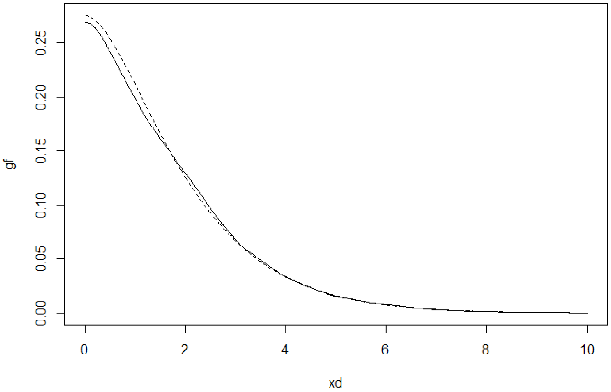
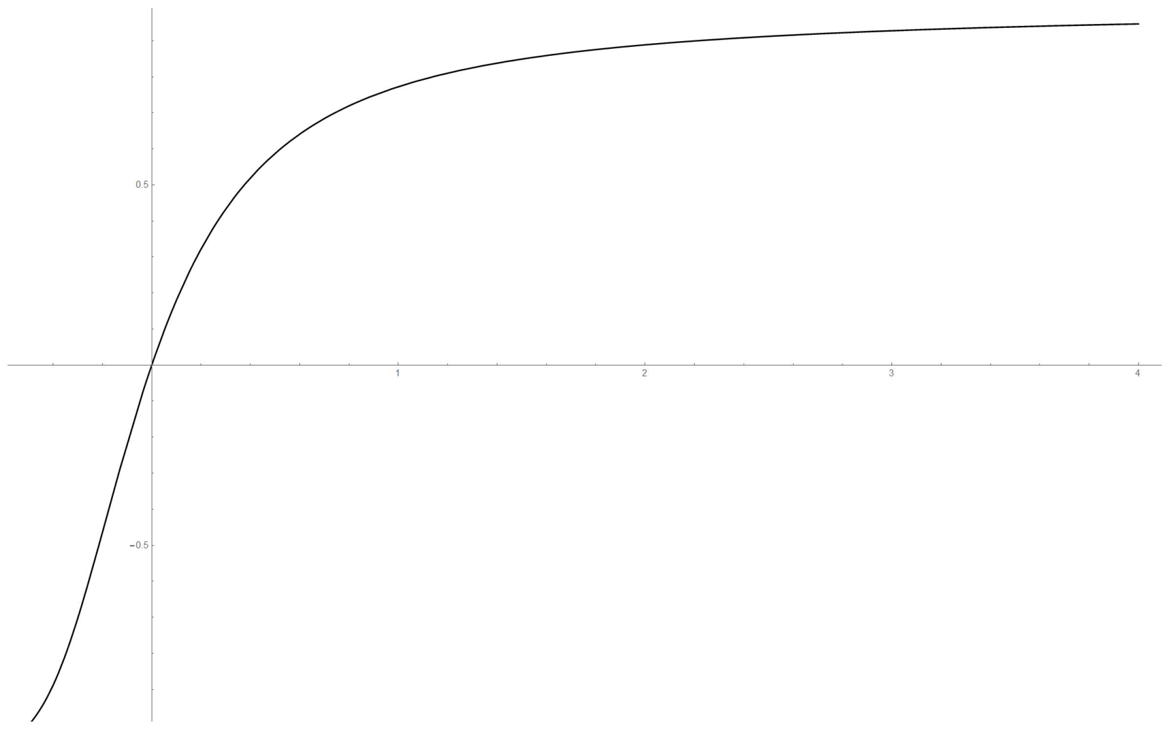
To illustrate how the estimators work in practice, we simulated data from a q-norm distribution with $q=1.3$ and the radius distribution to be the modified exponential distribution with $\tau =1.1$. The Figure 7 and Figure 8 include graphs of the underlying function g and its estimator in two cases.

Figure 7. Estimator of g (solid line) and the model function (dashed line) for $n=1000$.

Figure 8. Estimator of g (solid line) and the model function (dashed line) for $n=\mathrm{10,000}$.

3.2.5. Reference Bandwidth

Let us consider an estimator ${\widehat{\phi }}_n(x)$ with Epanechnikov kernel, function ψ as in Example 10, and modified exponential radius density in the case $p=2$. According to (16), the reference bandwidth is then

$$b^{*}={\left(15(d+1)(d-1)!e^{\tilde{x}/\tau }{\tilde{x}}^{4d}{\tau }^{5/d}{(1+{\tilde{x}}^d)}^{-1+5/d}(\tilde{x}+\tau ){\left({\mathcal{O}}_S(S)D^{2}n\right)}^{-1}\right)}^{1/5},$$

where

$$\begin{array}{ccc}\hfill D& =& {\tilde{x}}^2(\tilde{x}+(d-2)\tau )+{\tilde{x}}^{d+2}(2\tilde{x}-(d+1)\tau )\hfill \\ & & +{\tilde{x}}^{2d}\left({\tilde{x}}^3+(d-2)(d-1)(\tilde{x}+\tau ){\tau }^2+{\tilde{x}}^2\tau (1-2d)\right).\hfill \end{array}$$

This formula was generated using the computer algebra system Mathematica. The parameter τ can be estimated by utilizing the above Formula (6) for the expectation of the radius.

3.3. Semiparametric Estimators Involving a Scale and a Parameter Fit

In this section we consider the situation where the contour of the body K depends on scale parameters ${\sigma }_1,\dots ,{\sigma }_d$. Suppose that $I(g,d)=1$. We introduce the diagonal matrix $\mathrm{\Sigma }=diag({\sigma }_1,\dots ,{\sigma }_d)$ and a master body $K_0$, which is symmetric w.r.t. the origin. Define

$$K=\mathrm{\Sigma }{K}_0:=\{\mathrm{\Sigma }x:x\in K_0\},$$

and $\tilde{U}={\mathrm{\Sigma }}^{-1}U$. The distribution of $\tilde{U}$ is concentrated on the boundary $S_0$ of $K_0$. We assume that $K_0$ is given such that

$$\mathbb{E}{\tilde{U}}_j^2=1\mathrm{for}j=1,\dots ,d.$$

(17)

Otherwise, $K_0$ is rescaled. Suppose that $h_{K_0}$ depends on a further parameter vector $\theta \in \mathrm{\Theta }$ where the parameter space $\mathrm{\Theta }\subset {\mathbb{R}}^q$ is a compact set. Then

$$h_K(x)=h_{K_0}(\theta ,{\mathrm{\Sigma }}^{-1}x)\mathrm{for}x\in {\mathbb{R}}^d.$$

The parameter vector θ is able to describe the shape of the boundary of body K, see Examples 1 and 2 (parameters $a_1$ and $a_2$). From Lemma 1, we obtain

$$\begin{array}{ccc}\hfill \mathbb{V}(X^{(j)})& =& {\sigma }_j^2\mathbb{E}{\tilde{U}}_j^2\mathbb{E}{R}^2={\sigma }_j^2\mathbb{E}{R}^2,\hfill \\ \hfill \mathbb{C}\mathbf{ov}(X^{(j)},X^{(k)})& =& {\sigma }_j{\sigma }_k\mathbb{E}{\tilde{U}}_j{\tilde{U}}_k\mathbb{E}{R}^2,\hfill \end{array}$$

and

$${\rho }_{jk}=\mathbb{C}\mathbf{orr}(X^{(j)},X^{(k)})=\mathbb{E}{\tilde{U}}_j{\tilde{U}}_k\mathrm{for}j,k=1,\dots ,d.$$

Here we see that (17) results in $\mathbb{V}(X^{(j)})={\sigma }_j^2\mathbb{E}{R}^2$. The density is given by

$${\phi }_{g,K,\mu }(x)={\mathcal{O}}_{S_0}{(S_0)}^{-1}det{(\mathrm{\Sigma })}^{-1}g\left(h_{K_0}(\theta ,{\mathrm{\Sigma }}^{-1}(x-\mu ))\right),x\in {\mathbb{R}}^d.$$

In this context, a scaling problem occurs concerning g. Assume that g is a suitably given generator function satisfying $I(g,d)=1$. Then $x⇝g_t^{*}(x):=t^{d-1}g(tx)$ is a modified generator for every $t\in \mathbb{R}$ with $I(g_t^{*},d)=1$. For any $t\in \mathbb{R}$, we obtain the same model when g is replaced by $g_t^{*}$ and ${\sigma }_j$ is replaced by ${\sigma }_{j}t$ for $j=1,\dots ,d$. To get uniqueness, we choose t such that

$$\mathbb{E}{R}^2={\int }_0^{\infty }{r}^{d+1}{g}_t^{*}(r)dr=t^{-2}{\int }_0^{\infty }{r}^{d+1}g(r)dr=1.$$

Let ${\widehat{\mu }}_n={({\widehat{\mu }}_{n1},\dots ,{\widehat{\mu }}_{nd})}^T$ as above. Then ${\sigma }_j^2$ represents the variance of the j-th component of X. Based on this property, the sample variances of the components of X can be used as estimators for ${\sigma }_j^2$:

$${\widehat{\sigma }}_{nj}^2=\frac{1}{n-1}\sum _{i=1}^n{\left(X_{ij}-{\widehat{\mu }}_{nj}\right)}^2\mathrm{for}j=1,\dots ,d.$$

Moreover, we have the sample correlations

$${\widehat{\rho }}_{njk}={\widehat{\sigma }}_j^{-1}{\widehat{\sigma }}_k^{-1}\frac{1}{n-1}\sum _{i=1}^n\left(X_{ij}-{\widehat{\mu }}_{nj}\right)\left(X_{ik}-{\widehat{\mu }}_{nk}\right)\mathrm{for}j,k=1,\dots ,d.$$

In the following we use the notation ${\widehat{\mathrm{\Sigma }}}_n=$ diag$({\widehat{\sigma }}_{n1},\dots ,{\widehat{\sigma }}_{nd})$. If θ is unknown, we consider moment estimators based on the correlations. For this we need the following assumptions.

Assumption 6.

Let I be a subset of $\{(j,k):j,k=1,\dots ,d,j<k\}$ with cardinality q. There is a vector $\rho ={({\rho }_{jk})}_{(j,k)\in I}\in {\mathbb{R}}^q$ such that for $l=1,\dots ,q$,

$${\theta }_l={\gamma }_l(\rho ).$$

Assume that ${\gamma }_l:\mathcal{C}\to \mathrm{\Theta }$ has bounded partial derivatives, $\rho \in \mathcal{C}$ and θ is an interior point of Θ.

Assumption 7.

For any bounded subset Q of ${\mathbb{R}}^d,0\notin Q$, the partial derivatives ${\tilde{G}}_1,\dots ,{\tilde{G}}_q$, $G_1,\dots ,G_d$ of $(\theta ,x)⇝h_{K_0}(\theta ,x)$ exist, are bounded for $\theta \in \mathrm{\Theta },x\in Q$, and $(\theta ,x)⇝{\psi }^{\prime }(h_{K_0}(\theta ,x))G_j(\theta ,x)$, ${\psi }^{\prime }(h_{K_0}(\theta ,x)){\tilde{G}}_j(\theta ,x)$ is Hölder continuous of order $\alpha >0.2$ on $\mathrm{\Theta }\times Q$ for each $j\in \{1,\dots ,d\}$.

Assumption 8.

For any bounded subset Q of ${\mathbb{R}}^d,0\notin Q$, $h_{K_0}$ is Hölder continuous of order $\overline{\alpha }>0.2$.

Examples 1 and 2: (Continued) Similarly as above, it can be proven that Assumption 7 is fulfilled.

Let $\widehat{\rho }$ be the sample version of ρ. Then

$${\widehat{\theta }}_{nl}={\gamma }_l(\widehat{\rho })\mathrm{for}l=1,\dots ,q$$

is the estimator for θ, ${\widehat{\theta }}_n={({\widehat{\theta }}_{nl})}_{l=1\dots q}$. Define ${\widehat{R}}_i={\widehat{\mathrm{\Sigma }}}^{-1}(X_i-{\widehat{\mu }}_n)$. With this definition, ${\widehat{F}}_n^R$ is determined according to Formula (8). The following result on the convergence rate of ${\widehat{F}}_n^R$ can be proven:

Theorem 4.

Suppose that Assumptions 1 and 6 are satisfied, and

$${\int }_0^{\infty }{r}^{d+3}g(r)dr<+\infty .$$

(18)

Let $r⇝r{f}_R(r)$ be bounded on $[0,+\infty )$. Then, for $n\to \infty$,

$$\underset{r\ge 0}{sup}\left|{\widehat{F}}_n^R(r)-F_R(r)\right|=O\left(\sqrt{\frac{lnln(n)}{n}}\right)a.s.$$

In this section the transformed sample $Y_{1n},\dots ,Y_{nn}$ is given by $Y_{in}=\psi (h_{K_0}({\widehat{\theta }}_n,{\widehat{R}}_i))$ with ψ as in Section 3.2. The estimator ${\widehat{g}}_n$ for the generator g is calculated using Formulas (10) and (11) from the previous section. The following estimator for the density has thus been established:

$${\widehat{\phi }}_n(x)={\mathcal{O}}_{S_0}{(S_0)}^{-1}det{({\widehat{\mathrm{\Sigma }}}_n)}^{-1}{\widehat{g}}_n\left(h_{K_0}({\widehat{\theta }}_n,{\widehat{\mathrm{\Sigma }}}_n^{-1}(x-{\widehat{\mu }}_n))\right)$$

(19)

The next two theorems show the results concerning strong convergence and asymptotic normality of the density estimator:

Theorem 5.

Suppose that the p-th order derivative $g^{(p)}$ of g exists and is bounded on $[0,\infty )$ for some even integer $p\ge 2$. Where needed, with this p, assume further that Assumptions 1, 2, 3, 6, (1) and (18) are satisfied. Let Assumption 7 or Assumption 8 be satisfied, and define in the first case $r_n:=\sqrt{lnn}{(nb)}^{-1/2}$ and in the latter case $r_n:=n^{-\overline{\alpha }/2}{b}^{-1}$.Then the claim of Theorem 2 holds true for estimator ${\widehat{\phi }}_n$ defined in (19).

Theorem 6.

Suppose that the assumptions of Theorem 5 are satisfied. Let $x\in {\mathbb{R}}^d,x\ne \mu$ such that $g^{(p)}$ is continuous at $\tilde{x}:=h_{K_0}(\theta ,{\mathrm{\Sigma }}^{-1}(x-\mu ))$. Assume that ${lim}_{n\to \infty }{n}^{1/(2p+1)}b=C_4$ holds true with a constant $C_4\ge 0$. Then for $n\to \infty$,

$$\sqrt{nb}\left({\widehat{\phi }}_n(x)-{\phi }_{g,K,\mu }(x)\right)\stackrel{d}{⟶}\mathcal{N}(C_4^{(2p+1)/2}\mathrm{\Lambda }(\tilde{x}),{\overline{\sigma }}^2(\tilde{x})),$$

where ${\widehat{\phi }}_n$ is defined in (19),

$$\begin{array}{ccc}\hfill {\overline{\sigma }}^2(\tilde{x})& =& {\mathcal{O}}_{S_0}{(S_0)}^{-2}det{(\mathrm{\Sigma })}^{-2}{\tilde{x}}^{1-d}{\psi }^{\prime }(\tilde{x})g(\tilde{x}){\int }_{-1}^1{k}^2(t)dt,\hfill \\ \hfill \mathrm{\Lambda }(\tilde{x})& =& {\mathcal{O}}_{S_0}{(S_0)}^{-1}det{(\mathrm{\Sigma })}^{-1}{\tilde{x}}^{1-d}{\psi }^{\prime }(\tilde{x})\frac{1}{p!}{\chi }^{(p)}(\psi (\tilde{x})){\int }_{-1}^1{t}^{p}k(t)dt.\hfill \end{array}$$

The remarks following Theorems 2 and 3 are valid similarly.

3.4. Applications

For many decades, statistical applications of multivariate distribution theory were manly based upon Gaussian and elliptically contoured distributions. Studies using non-elliptically contoured star-shaped distributions were basically made during the last two decades and are dealing in most cases with p-generalized normal distributions. Such distributions are convex or radially concave contoured if $p\ge 1$ or $0<p\le 1,$ respectively, and are also called power exponential distributions. Moreover, common elliptically contoured power exponential (ecpe) distributions build a particular class of the wide class of star-shaped distributions that allows modeling much more flexible contours than elliptically ones.

The class of ecpe distributions is used in a crossover trial on insulin applied to rabbits in [23], in image denoising in [24] and in colour texture retrieval in [25]. Applications of multivariate g-and-h distributions to jointly modeling body mass index and lean body mass are demonstrated in [26] and accompanied by star-shaped contoured density illustrations. The $l_{n,p}$-elliptically contoured distributions build another big class of star-shaped distributions and are used in [27] to explore to which extent orientation selectivity and contrast gain control can be used to model the statistics of natural images. Mixtures of ecpe distributions are considered for bioinformation data sets in [28]. Texture retrieval using the p-generalized Gaussian densities is studied in [29]. A random vector modeling data from quantitative genetics presented in [30] are shown in [31] to be more likely to have a power exponential distribution different from a normal one. The reconstruction of the signal induced by cosmic strings in the cosmic microwave background, from radio-interferometric data, is made in [32] based upon generalized Gaussian distributions. These distributions are also used in [33] for voice detection.

More recently, the considerations in [11] opened a new field of financial applications of more general star-shaped asymptotic distributions, where suitably scaled sample clouds converge onto a deterministic set.

Figure 3 in [34] represents a sample cloud which might be modeled with a density being star-shaped w.r.t. a fan having six cones that include sample points and other cones that do not. Note, however, that Figure 1 d-f in the same paper do not reflect a homogeneous density but might be compared in some sense to the level sets of the characteristic functions of certain polyhedral star-shaped distributions in [16], Figure 5.2.

When modeling Lymphoma data, [35] analyze sample clouds of points, see Figures 2 and 3, which might be interpreted as mixtures of densities having contours in part looking similar like that in [36] where flow cytometric data, Australian Institute of Sport data and Iris data are analyzed, or like that of certain skewed densities as they were (analytically derived and) drawn in [37]. In a similar manner, Figures 2 and 5 in [20] indicate that mixtures of different types of star-shaped distributions might be suitable for modeling residuals of certain stock exchange indices. It could be of interest to closer study in future work more possible connections of all the models behind.

The following numerical examples of the present section are aimed to illustrate the agricultural and financial application of the estimators described in this paper. To this end, we make use of the new particular non-elliptically contoured but star-shaped distribution class introduced in Section 2.2 of the present paper.

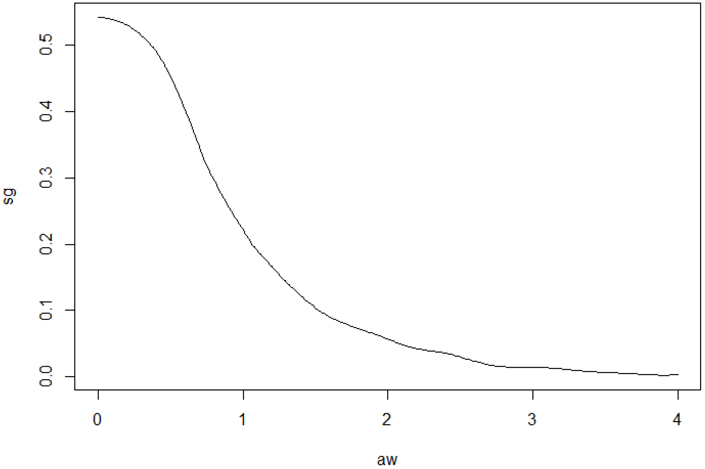
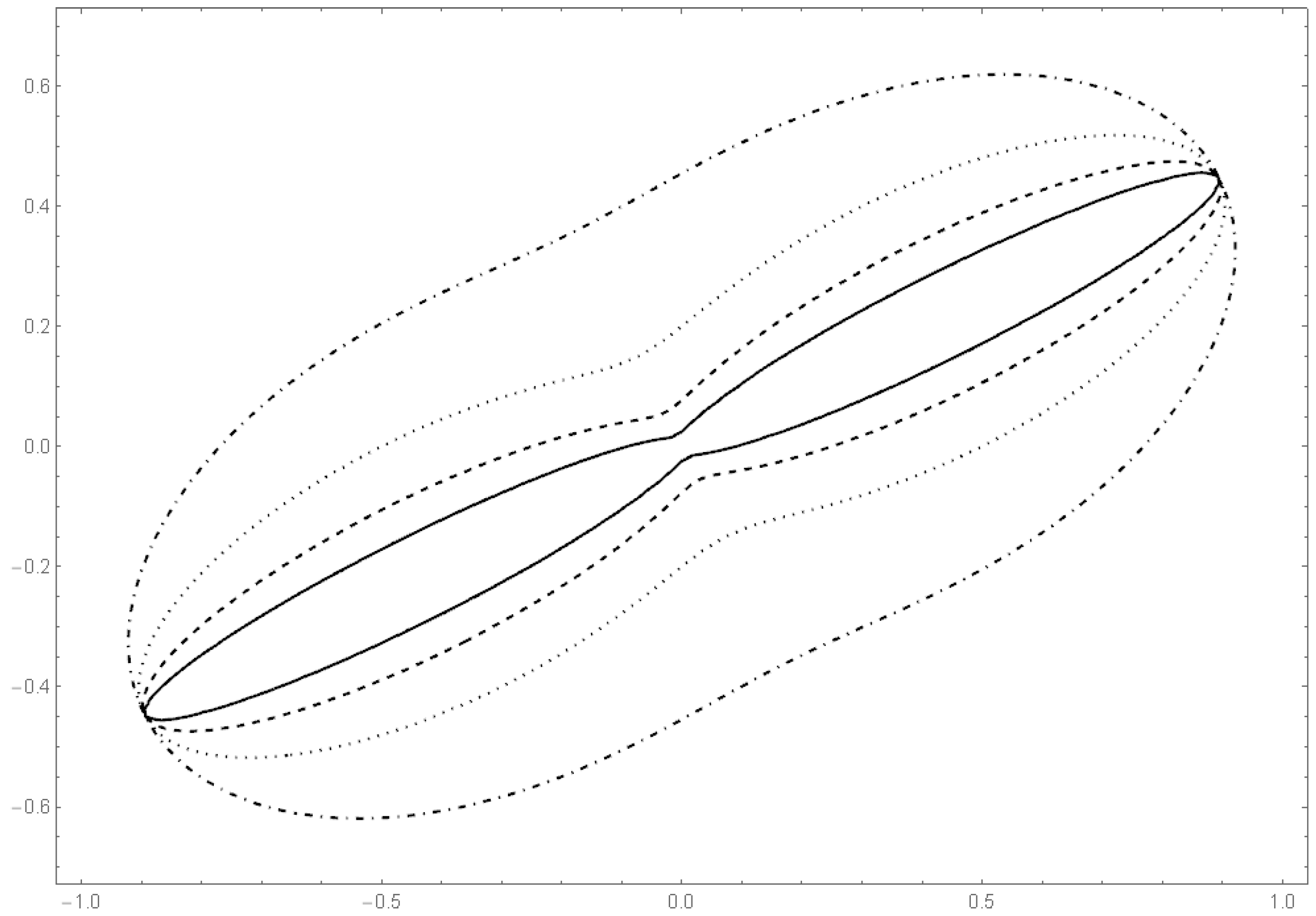
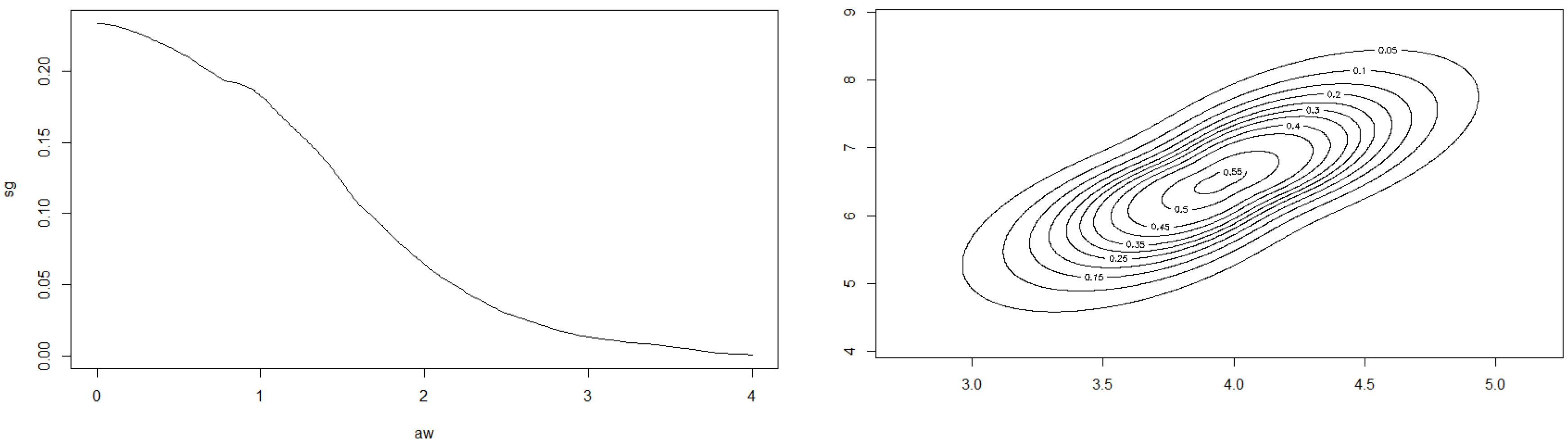
Example 12.

Example 2 of Section 2.2 continued. We consider the class of bodies K of Example 2. Let $a_2=1$. Figure 9 shows the dependence of the correlation on the parameter $a_1$.

Figure 9. Function ${\gamma }_1^{-1}$ with $a_1$ on the x-axis, ρ on the y-axis; ${\gamma }_1$ is defined in Assumption 6.

Here we apply the above described methods to the dataset 5 of [38]. The yield of grain and straw are the two variables. The sample correlation is 0.73077. Starting from that value, we can calculate the moment estimator for $a_1$: ${\widehat{a}}_1=0.83641$. Moreover, we obtain

$$\begin{array}{ccc}\hfill {\mathcal{O}}_{S_0}(S_0)& =& 2.6406,{\widehat{\mu }}_1=3.9480,{\widehat{\mu }}_2=6.5148\hfill \\ \hfill {\widehat{\sigma }}_1& =& 0.45798,{\widehat{\sigma }}_2=0.89831.\hfill \end{array}$$

The data and the shape of the estimated multivariate density are depicted in Figure 10 and Figure 11.

Figure 11. Estimated generator function g at left (bandwidth $b=0.5$) and contour plot of $\widehat{\phi }$ at right.

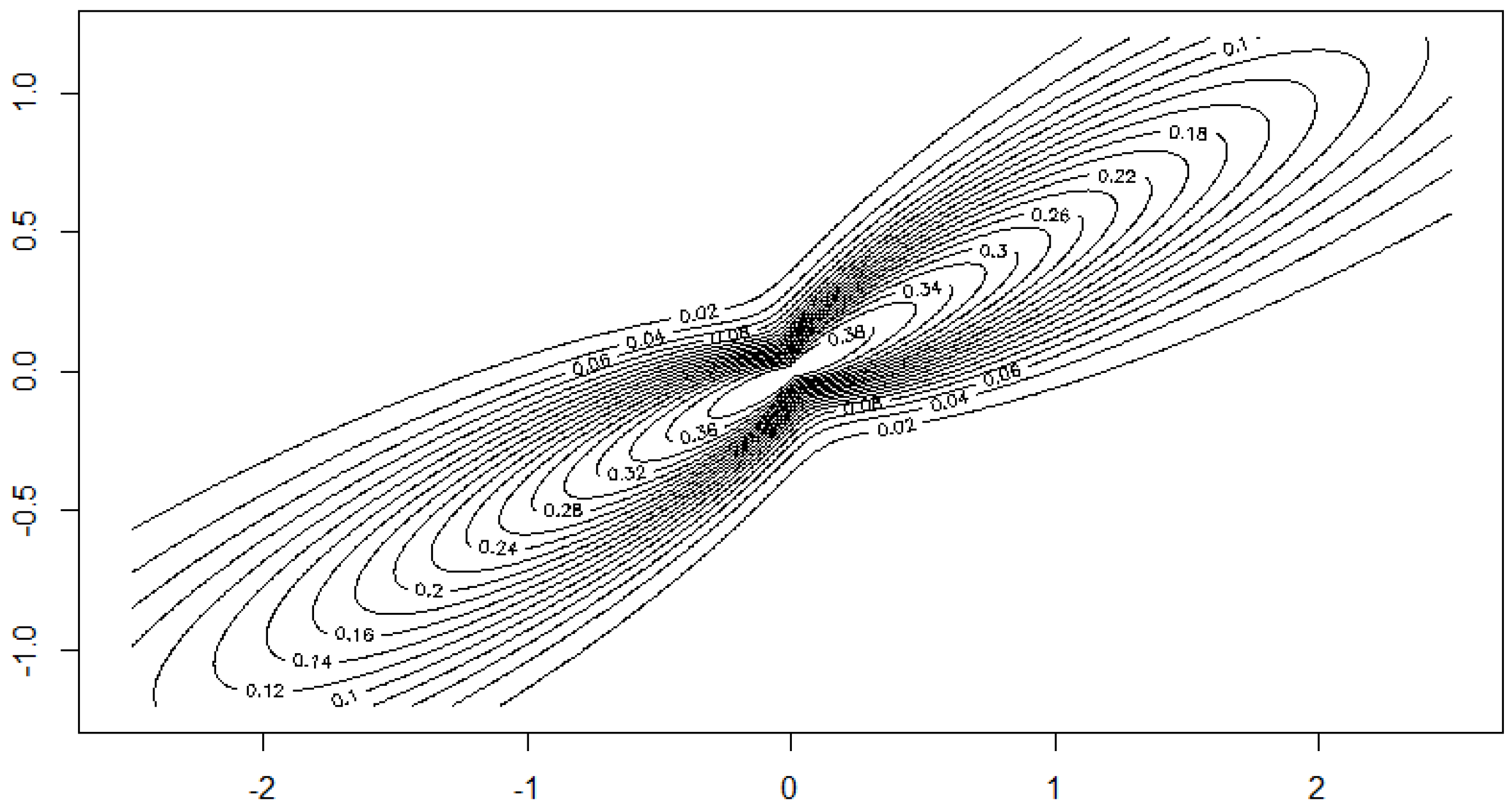
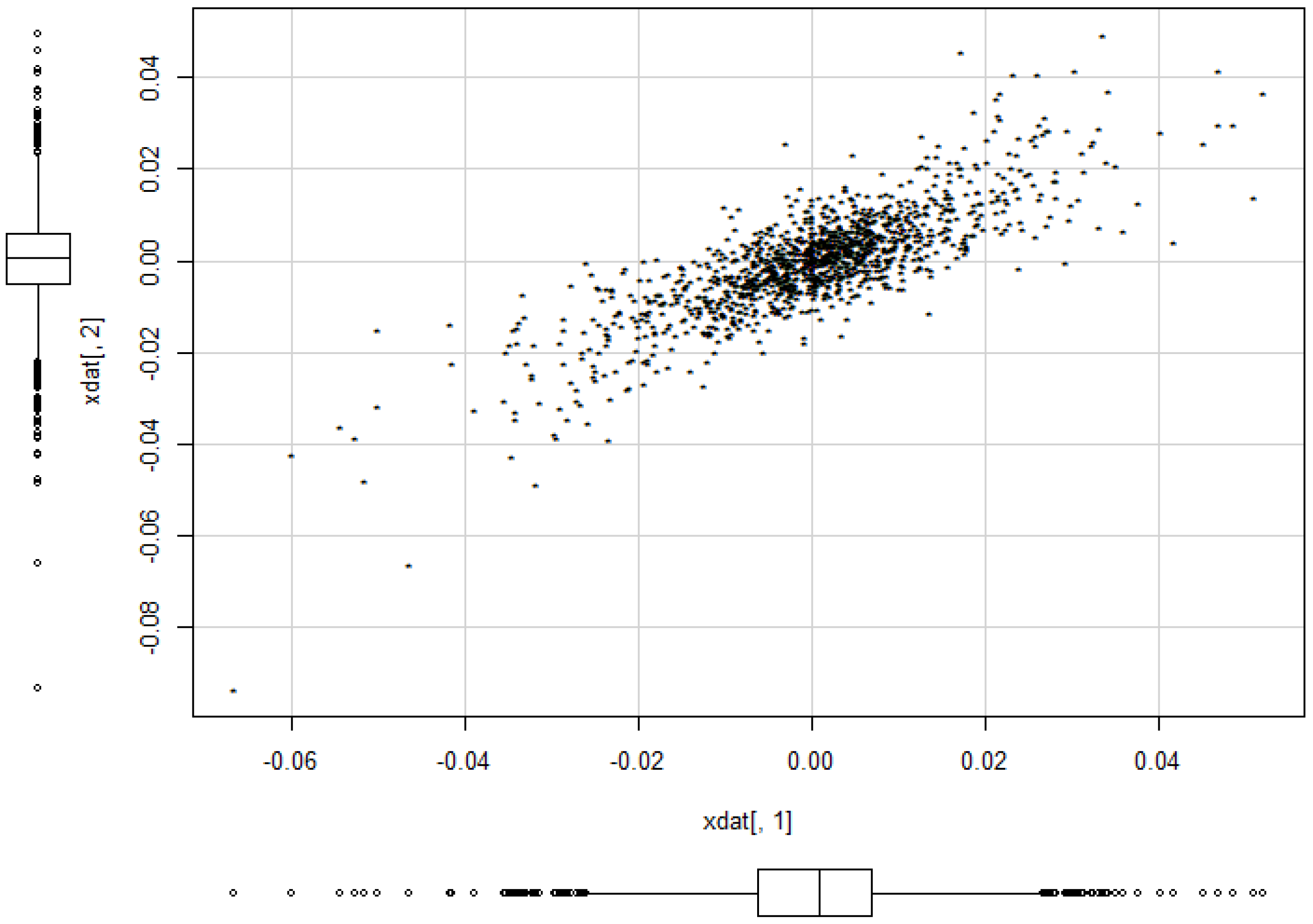
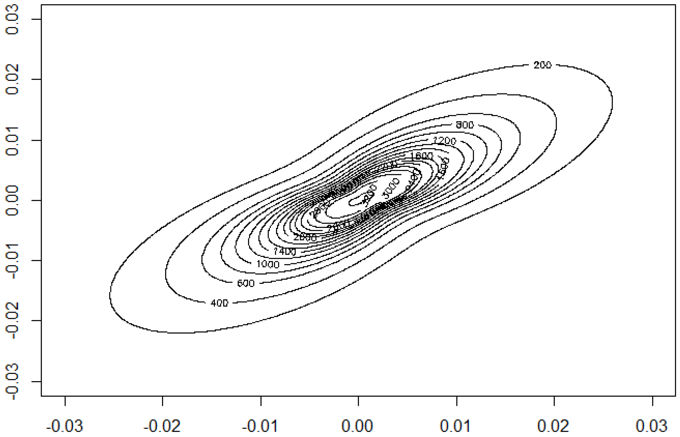
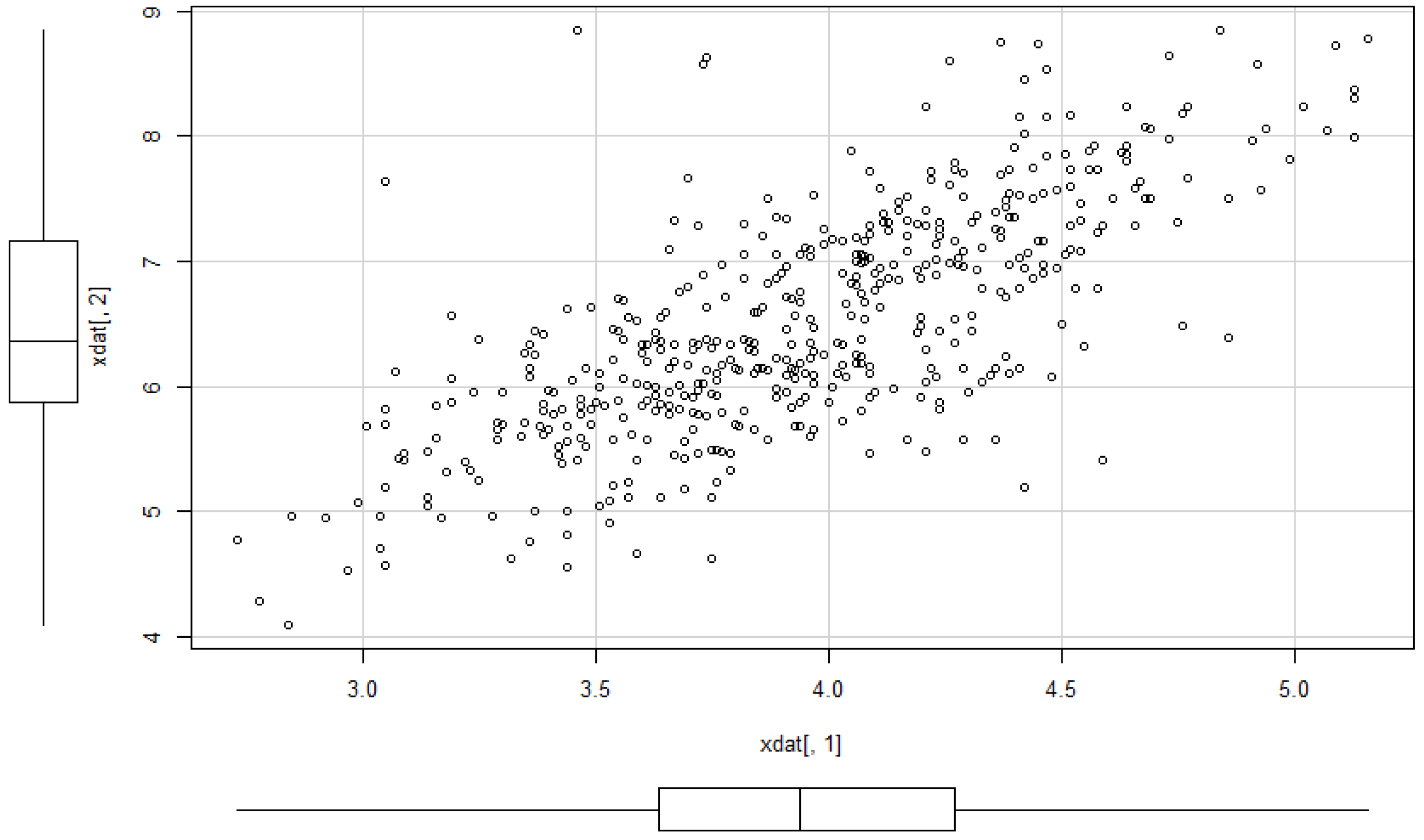
Example 13.

We want to illustrate the potential of our approach for applications to financial data and consider daily index data from Morgan Stanley Capital International of the countries Germany and UK for the period August 2011 to June 2016. The data indicate the continuous daily return values computed as logarithm of the ratio of two subsequent index values. The modelling of MSCI data using elliptical models is considered in [5]. The data are depicted in Figure 12. A visual inspection seems to give some preference for our model from Section 2.2 compared to the elliptically contoured model. Figure 13 and Figure 14 show the estimated model for the data. The basic numerical results are:

$$\begin{array}{ccc}\hfill {\mathcal{O}}_{S_0}(S_0)& =& 2.1966,{\widehat{a}}_1=1.2088,{\widehat{\mu }}_1=0.00026725,{\widehat{\mu }}_2=0.00026855\hfill \\ \hfill {\widehat{\sigma }}_1& =& 0.013519,{\widehat{\sigma }}_2=0.011715.\hfill \end{array}$$

Figure 12. Scatter plot of the MSCI data.

Figure 13. Contour plot of the estimated density.

Figure 14. Estimated generator function g (bandwidth $b=0.25$).

Further we proceed with proving the results.

4. Proofs

Throughout the remainder of the paper, suppose that Assumptions 1–3 are satisfied for some integer $p\ge 2$. First, we prove auxiliary statements which are used in the proof of strong convergence of ${\widehat{\phi }}_n$ and later.

4.1. Proof of Auxiliary Statements

The following Lemma 2 clarifies the asymptotic behaviour of χ in the neighbourhood of zero.

Lemma 2.

Suppose that $g^{\prime }$ exists and is bounded. Then

$$\underset{t,u\in [0,\overline{M}]}{sup}\left|\chi (t)-\chi (u)\right|{|t-u|}^{-1/d}<+\infty$$

for any $\overline{M}>0$.

Proof. 

Observe that by the Lipschitz continuity of the functions g and $z⇝z^{d-1}{\psi }^{\prime }{(z)}^{-1}$ in view of Assumption 3,

$$\begin{array}{ccc}& & \left|\chi (t)-\chi (u)\right|\hfill \\ & \le & C·\left(\frac{\mathrm{\Psi }{(t)}^{d-1}}{{\psi }^{\prime }(\mathrm{\Psi }(t))}\left|g(\mathrm{\Psi }(t))-g(\mathrm{\Psi }(u))\right|+\left|\frac{\mathrm{\Psi }{(t)}^{d-1}}{{\psi }^{\prime }(\mathrm{\Psi }(t))}-\frac{\mathrm{\Psi }{(u)}^{d-1}}{{\psi }^{\prime }(\mathrm{\Psi }(u))}\right|g(\mathrm{\Psi }(u))\right)\hfill \\ & \le & C·\left|\mathrm{\Psi }(t)-\mathrm{\Psi }(u)\right|\hfill \end{array}$$

(20)

uniformly for $t,v\in [0,\overline{M}]$. Here and in the following C is a generic constant which may differ from formula to formula. By assumption, we have

$$\left|{\mathrm{\Psi }}^d(t)-{\mathrm{\Psi }}^d(u)\right|\le C·|t-u|.$$

On the other hand,

$$\underset{t,u\ge 0}{sup}\frac{|t^{1/d}-u^{1/d}|}{{|t-u|}^{1/d}}<+\infty .$$

Hence

$$\left|\mathrm{\Psi }(t)-\mathrm{\Psi }(u)\right|\le C·{\left|{\mathrm{\Psi }}^d(t)-{\mathrm{\Psi }}^d(u)\right|}^{1/d}\le C·{|t-u|}^{1/d}.$$

In view of (20), the proof is complete. ☐

Lemma 3.

Let (9) be fulfilled. Then, for $n\to \infty$,

$${∥{\widehat{\mu }}_n-\mu ∥}_2=O\left(\sqrt{\frac{lnln(n)}{n}}\right)a.s.$$

If in addition (18) is satisfied then, for $n\to \infty$,

$$\underset{j=1,\dots ,d}{max}\left|{\widehat{\sigma }}_{nj}-{\sigma }_j\right|=O\left(\sqrt{\frac{lnln(n)}{n}}\right)a.s.$$

Proof. 

Because of (9), the law of iterated logarithm applies and leads to

$$\underset{n\to \infty }{limsup}\sqrt{\frac{n}{lnlnn}}\left|{\widehat{\mu }}_{nj}-{\mu }_j\right|=\sqrt{2\mathbb{V}{X}_j}a.s.$$

(21)

Since there is a constant $C>0$ such that ${∥y∥}_2\le C{∥y∥}_{\infty }$ for all $y\in {\mathbb{R}}^d$ in view of the norm equivalence property, the first part of the lemma follows from (21). The second part can be shown similarly. ☐

In several places, we will use the following property:

Lemma 4.

Suppose that $\mathrm{\Lambda }:{\mathbb{R}}^d\to \mathbb{R}$ is a measurable function with $\mathrm{\Lambda }(-x)=-\mathrm{\Lambda }(x)$. Then

$$\mathbb{E}\left(\mathrm{\Lambda }(X-\mu )\right)=0$$

Proof. 

Since $-X+\mu$ has the same distribution as $X-\mu$, we have

$$\begin{array}{ccc}\hfill \mathbb{E}\left(\mathrm{\Lambda }(X-\mu )\right)& =& \mathbb{E}\left(\mathrm{\Lambda }(X-\mu )\mathbf{1}\{X_1-{\mu }_1<0\}\right)+\mathbb{E}\left(\mathrm{\Lambda }(X-\mu )\mathbf{1}\{X_1-{\mu }_1>0\}\right)\hfill \\ & =& \mathbb{E}\left(\mathrm{\Lambda }(-X+\mu )\mathbf{1}\{X_1-{\mu }_1>0\}\right)+\mathbb{E}\left(\mathrm{\Lambda }(X-\mu )\mathbf{1}\{X_1-{\mu }_1>0\}\right)=0\hfill \end{array}$$

which proves the lemma. ☐

4.2. Proving Convergence of ${\widehat{F}}_n^R$

In this section we prove Theorem 1. The law of the iterated logarithm for the empirical process says (cf. [39], p. 268, for example)

$${\mathrm{\Delta }}_n:=\underset{r\in \mathbb{R}}{sup}\left|F_n^R(r)-F_R(r)\right|=O\left(\sqrt{\frac{lnln(n)}{n}}\right)a.s.$$

By Lipschitz-continuity of $h_K$ and Lemma 3,

$$\begin{array}{ccc}\hfill {\overline{\mathrm{\Delta }}}_n& :& =\underset{x\in {\mathbb{R}}^d}{sup}\left|h_K(x-{\widehat{\mu }}_n)-h_K(x-\mu )\right|\hfill \\ & \le & C{∥{\widehat{\mu }}_n-\mu ∥}_2=O\left(\sqrt{\frac{lnln(n)}{n}}\right)a.s.\hfill \end{array}$$

Moreover,

$$\begin{array}{ccc}\hfill {\widehat{F}}_n^R(r)-F_R(r)& =& \frac{1}{n}\sum _{i=1}^n\left(\mathbf{1}\left\{h_K(X_i-{\widehat{\mu }}_n)\le r\right\}-\mathbf{1}\left\{h_K(X_i-\mu )\le r\right\}\right)+F_n^R(r)-F_R(r)\hfill \\ & \le & \frac{1}{n}\sum _{i=1}^n\left(\mathbf{1}\left\{h_K(X_i-{\widehat{\mu }}_n)\le r,h_K(X_i-\mu )>r\right\}\right.\hfill \\ & & \left.-\mathbf{1}\left\{h_K(X_i-\mu )\le r,h_K(X_i-{\widehat{\mu }}_n)>r\right\}\right)+F_n^R(r)-F_R(r)\hfill \\ & \le & \frac{1}{n}\sum _{i=1}^n\mathbf{1}\left\{r<h_K(X_i-\mu )\le r+{\overline{\mathrm{\Delta }}}_n\right\}+{\mathrm{\Delta }}_n,\hfill \end{array}$$

and

$${\widehat{F}}_n^R(r)-F_R(r)\ge -\frac{1}{n}\sum _{i=1}^n\mathbf{1}\left\{r-{\overline{\mathrm{\Delta }}}_n<h_K(X_i-\mu )\le r\right\}-{\mathrm{\Delta }}_n.$$

Hence, by the boundedness of $f_R$,

$$\begin{array}{ccc}& & \underset{r\ge 0}{sup}\left|{\widehat{F}}_n^R(r)-F_R(r)\right|\hfill \\ & \le & \frac{1}{n}\underset{r\ge 0}{sup}\sum _{i=1}^n\mathbf{1}\left\{r-{\overline{\mathrm{\Delta }}}_n<h_K(X_i-\mu )\le r+{\overline{\mathrm{\Delta }}}_n\right\}+{\mathrm{\Delta }}_n\hfill \\ & =& \underset{r\ge 0}{sup}\left(F_n^R(r+{\overline{\mathrm{\Delta }}}_n)-F_n^R(r-{\overline{\mathrm{\Delta }}}_n)\right)+{\mathrm{\Delta }}_n\hfill \\ & \le & \underset{r\ge 0}{sup}\left(F_R(r+{\overline{\mathrm{\Delta }}}_n)-F_R(r-{\overline{\mathrm{\Delta }}}_n)\right)+3{\mathrm{\Delta }}_n\hfill \\ & \le & 2\underset{r\ge 0}{sup}{f}_R(r){\overline{\mathrm{\Delta }}}_n+O\left(\sqrt{\frac{lnlnn}{n}}\right)=O\left(\sqrt{\frac{lnlnn}{n}}\right)a.s.,\hfill \end{array}$$

which leads to the theorem. ☐

4.3. Proving Strong Convergence of the Density Estimator

Let ${\tilde{Y}}_i=\psi \left(h_K(X_i-\mu )\right)$ for $i=1,\dots ,n$, $K_b(y,t)=k((y-t)/b)+k((y+t)/b)$ for $y,t\ge 0$, $Y_{in}=\psi (h_K(X_i-{\widehat{\mu }}_n))$, and

$${\tilde{\chi }}_n(y)=\frac{1}{nb}\sum _{i=1}^n{K}_b(y,{\tilde{Y}}_i)$$

for $y\ge 0$. Then (cf. (10))

$${\widehat{\chi }}_n(y)=\frac{1}{nb}\sum _{i=1}^n{K}_b(y,Y_{in}).$$

Next we prove strong convergence rates for ${\widehat{\chi }}_n$ and later for ${\widehat{\phi }}_n$. Throughout this section we suppose that Assumptions 1 to 3 and (9) are fulfilled for some even integer $p\ge 2$. The compact set $[m,M]$ with arbitrary m and M, $0\le m<M$ can be covered with closed intervals $U_1,\dots ,U_n$ having sides of length $(M-m)n^{-1}$ and centres $u_1,\dots ,u_n$ such that ${\bigcup }_{i=1}^n{U}_i=[m,M]$. The constants m and M will be specified later. Note that

$$\begin{array}{ccc}\hfill \underset{y\in [m,M]}{sup}\left|{\widehat{\chi }}_n(y)-\chi (y)\right|& \le & \underset{l=1,\dots ,n}{max}\left(\underset{y\in U_l}{sup}\left|{\widehat{\chi }}_n(y)-{\widehat{\chi }}_n(u_l)\right|+\left|{\widehat{\chi }}_n(u_l)-{\tilde{\chi }}_n(u_l)\right|\right.\hfill \\ & & \left.+\left|{\tilde{\chi }}_n(u_l)-\chi (u_l)\right|+\underset{y\in U_l}{sup}\left|\chi (u_l)-\chi (y)\right|\right).\hfill \end{array}$$

(22)

The asymptotic behaviour of the right hand side in (22) as $n\to \infty$ is analyzed term by term in the next lemmas.

Lemma 5.

Assume that the p-th order derivative ${\chi }^{(p)}$ of χ exists for some even integer $p\ge 2$ and is bounded on every finite closed subinterval of $(0,\infty )$. Let $g^{\prime }$ be bounded. Then

$$\underset{l=1,\dots ,n}{max}\left|{\tilde{\chi }}_n(u_l)-\chi (u_l)\right|=O\left(\sqrt{lnn}{(nb)}^{-1/2}+{\beta }_n\right)a.s.$$

where ${\beta }_n=b^p$ if $m>0$ and ${\beta }_n=b^{1/d}$ if $m=0$.

The proof of this lemma is omitted since, with minor changes, this lemma can be proven in the same way as Lemma 4.4 in [7]. The following lemma is used later several times in proofs of almost sure convergence rates. We provide it without proof. The proof is almost identical to that of Lemma 4.6 in [7].

Lemma 6.

Assume that χ is bounded. Let $\overline{k},\lambda :\mathbb{R}\to \mathbb{R}$ be bounded measurable functions with $\overline{k}(t)=0$ for $t:\left|t\right|>1$. Then

$$\begin{array}{ccc}\hfill \underset{l=1,\dots ,n}{max}\left|\sum _{i=1}^n\left(U_{nil}-\mathbb{E}{U}_{nil}\right)\right|& =& O\left(\sqrt{nbln(n)}\right)a.s.,\hfill \\ \hfill \underset{l=1,\dots ,n}{max}\left|\sum _{i=1}^n\left({\overline{U}}_{nil}-\mathbb{E}{\overline{U}}_{nil}\right)\right|& =& O\left(\sqrt{nbln(n)}\right)a.s.,\hfill \\ \hfill \underset{l=1,\dots ,n}{max}\left|\sum _{i=1}^n\left(V_{nil}-\mathbb{E}{V}_{nil}\right)\right|& =& O\left(\sqrt{nbln(n)}\right)a.s.\hfill \end{array}$$

• where $U_{nil}:=\overline{k}((u_l-{\tilde{Y}}_i)/b)\mathbf{1}\{|{\tilde{Y}}_i-u_l|\le b-w_n\}\lambda (X_i)$,
• ${\overline{U}}_{nil}:=\overline{k}((u_l+{\tilde{Y}}_i)/b)\mathbf{1}\{|{\tilde{Y}}_i-u_l|\le b-w_n\}\lambda (X_i)$,
• $V_{inl}:=\mathbf{1}\{b-w_n<|{\tilde{Y}}_i-u_l|<b+w_n\}$.

We proceed with proving convergence rates of the terms in (22).

Lemma 7.

Suppose that Assumption 4 or 5 is satisfied. Then, as $n\to \infty ,$

$$\underset{l=1,\dots ,n}{max}\left|{\widehat{\chi }}_n(u_l)-{\tilde{\chi }}_n(u_l)\right|=\left\{\begin{array}{c}o\left({(nb)}^{-1/2}\right)\mathit{under}\mathit{Assumption}4,\hfill \\ O(b^{-1}{\left(n^{-1}lnlnn\right)}^{\overline{\alpha }/2})\mathit{under}\mathit{Assumption}5\hfill \end{array}\right.a.s.$$

Proof. 

(a) Let Assumption 4 be satisfied. In view of Lemma 3, we obtain

$$\begin{array}{ccc}\hfill \left|Y_{in}-{\tilde{Y}}_i\right|& \le & \underset{t\in [0,\infty )}{sup}\left|{\psi }^{\prime }(t)\right|\left|h_K(X_i-{\widehat{\mu }}_n)-h_K(X_i-\mu )\right|\hfill \\ & \le & C_5·\sqrt{\frac{lnlnn}{n}}=:w_n\hfill \end{array}$$

with a suitable constant $C_5>0$ for $n\ge n_1(\omega )$. We introduce

$${\kappa }_n(u,t)=\left(k^{\prime }((u-t)/b)-k^{\prime }((u+t)/b)\right)\mathbf{1}\left(\left|u-t\right|\le b-w_n\right).$$

Let $\overline{\psi }(z):=z^{-1}{\psi }^{\prime }(z)$. Observe that $k^{\prime }$ is bounded and Lipschitz continuous on $[-1,1]$, ${\psi }^{\prime },\overline{\psi }$ and ${\overline{\psi }}^{\prime }$ are bounded on $[0,+\infty )$, functions $G_j$ are bounded, and functions ${\psi }^{\prime }(h_K(.))G_j$ are Hölder continuous of order $\alpha >0.2$. We have then by Taylor expansion

$$\begin{array}{ccc}& & k\left(\frac{u-Y_{in}}{b}\right)+k\left(\frac{u+Y_{in}}{b}\right)-k\left(\frac{u-{\tilde{Y}}_i}{b}\right)-k\left(\frac{u+{\tilde{Y}}_i}{b}\right)\hfill \\ & =& -\frac{1}{b}\left(k^{\prime }((u-{\tilde{Y}}_i)/b)-k^{\prime }((u+{\tilde{Y}}_i)/b)\right){\psi }^{\prime }(h_K({\overline{X}}_i))\hfill \\ & & \times \sum _{j=1}^d{G}_j({\overline{X}}_i)\left({\widehat{\mu }}_{nj}-{\mu }_j\right)\mathbf{1}\left\{\left|{\tilde{Y}}_i-u\right|\le b-w_n\right\}+W_{ni}(u),\hfill \end{array}$$

where

$$\begin{array}{ccc}\hfill \left|W_{ni}(u)\right|& \le & C\left(b^{-2}{w}_n^2+b^{-1}{w}_n^{1+\alpha }\right)\mathbf{1}\left\{\left|{\tilde{Y}}_i-u\right|\le b-w_n\right\}\hfill \\ & & +C{b}^{-1}{w}_n\mathbf{1}\left\{b-w_n<\left|{\tilde{Y}}_i-u\right|<b+w_n\right\}a.s.\hfill \end{array}$$

uniformly w.r.t. $u\in [0,M]$. Here we have used Assumption 4 and Lipschitz continuity of k on $\mathbb{R}$. This leads to

$$\underset{l=1,\dots ,n}{max}\left|{\widehat{\chi }}_n(u_l)-{\tilde{\chi }}_n(u_l)\right|\le C\sum _{j=1}^d{B}_{1nj}\left|{\widehat{\mu }}_{nj}-{\mu }_j\right|+B_{2n}+B_{3n},$$

(23)

where

$$\begin{array}{ccc}\hfill B_{1nj}& =& n^{-1}{b}^{-2}\underset{l=1,\dots ,n}{max}\left|\sum _{i=1}^n{\kappa }_n(u_l,{\tilde{Y}}_i){\psi }^{\prime }(h_K({\overline{X}}_i))G_j({\overline{X}}_i)\right|,\hfill \\ \hfill B_{2n}& =& C\left(b^{-3}{w}_n^2+b^{-2}{w}_n^{1+\alpha }\right)\underset{l=1,\dots ,n}{max}\sum _{i=1}^n\mathbf{1}\left\{\left|{\tilde{Y}}_i-u_l\right|\le b-w_n\right\},\hfill \\ \hfill B_{3n}& =& C{n}^{-1}{b}^{-2}{w}_n\underset{l=1,\dots ,n}{max}\sum _{i=1}^n\mathbf{1}\left\{b-w_n<\left|{\tilde{Y}}_i-u_l\right|<b+w_n\right\}a.s.\hfill \end{array}$$

Note that

$$\begin{array}{ccc}\hfill B_{1nj}& =& n^{-1}{b}^{-2}\underset{l=1,\dots ,n}{max}\left|\sum _{i=1}^n{\kappa }_n(u_l,{\tilde{Y}}_i){\psi }^{\prime }(h_K({\overline{X}}_i))G_j({\overline{X}}_i)\right.\hfill \\ & & \left.-\sum _{i=1}^n\mathbb{E}\left({\kappa }_n(u_l,\psi (h_K({\overline{X}}_i))){\psi }^{\prime }(h_K({\overline{X}}_i))G_j({\overline{X}}_i)\right)\right|\hfill \end{array}$$

since the expectation in the last term is zero in view of Lemma 4 ($G_j(-x)=-G_j(x)$ holds for all $x\in {\mathbb{R}}^d$). Applying Lemma 6, it follows that

$$\sum _{j=1}^d{B}_{1nj}\left|{\widehat{\mu }}_{nj}-{\mu }_j\right|\le C{n}^{-3/2}{b}^{-2}\sqrt{lnlnn}·\sqrt{nblnn}=o\left({(nb)}^{-1/2}\right).$$

(24)

On the other hand, we obtain

$$\begin{array}{ccc}\hfill B_{2n}& \le & C\frac{lnlnn}{n^2{b}^3}\left(1+b{n}^{(1-\alpha )/2}\right)\underset{l=1,\dots ,n}{max}\sum _{i=1}^{n}I\left(\left|{\tilde{Y}}_i-u_l\right|\le b-w_n\right)\le C\frac{lnlnn}{n^2{b}^3}\left(1+b{n}^{(1-\alpha )/2}\right)\hfill \\ & & \left(\underset{l=1,\dots ,n}{max}\left|\sum _{i=1}^n\left(\mathbf{1}\left\{\left|{\tilde{Y}}_i-u_l\right|\le b-w_n\right\}-\mathbb{P}\left\{\left|{\tilde{Y}}_i-u_l\right|\le b-w_n\right\}\right)\right|\right.\hfill \\ & & \left.+n·\underset{v\in [0,\infty )}{sup}\mathbb{P}\left\{v\le {\tilde{Y}}_i\le v+2b-2w_n\right\}\right)\hfill \\ & \le & C\frac{lnlnn}{n^2{b}^3}\left(1+n^{(1-\alpha )/2}b\right)\left(\sqrt{nblnn}+nb\right)\hfill \\ & \le & Clnlnn\left(n^{-1}{b}^{-2}+n^{-(1+\alpha )/2}{b}^{-1}\right)=o\left({(nb)}^{-1/2}\right)a.s.,\hfill \end{array}$$

(25)

by utilizing Lemma 6 and taking $\alpha >0.2$ into account. Similarly, it follows that

$$\begin{array}{ccc}\hfill B_{3n}& \le & C\sqrt{\frac{lnlnn}{n^3{b}^4}}\underset{l=1,\dots ,n}{max}\sum _{i=1}^n\mathbf{1}\left\{b-w_n\le \left|{\tilde{Y}}_i-u_l\right|\le b+w_n\right\}\hfill \\ & \le & C\sqrt{\frac{lnlnn}{n^3{b}^4}}\underset{l=1,\dots ,n}{max}\left(\left|\sum _{i=1}^n\left(\mathbf{1}\left\{b-w_n\le \left|{\tilde{Y}}_i-u_l\right|\le b+w_n\right\}\right.\right.\right.\hfill \\ & & \left.\left.-\mathbb{P}\left\{b-w_n\le \left|{\tilde{Y}}_i-u_l\right|\le b+w_n\right\}\right)\right|+n·\mathbb{P}\left\{u_l+b-w_n<{\tilde{Y}}_i\le u_l+b+w_n\right\}\hfill \\ & & \left.+n·\mathbb{P}\left\{u_l-b-w_n<{\tilde{Y}}_i\le u_l-b+w_n\right\}\right)\hfill \\ & =& C\sqrt{\frac{lnlnn}{n^3{b}^4}}\left(\sqrt{nblnn}+n{w}_n\right)\hfill \\ & =& o\left({(nb)}^{-1/2}\right)a.s.\hfill \end{array}$$

(26)

Therefore, an application of (23)–(26) leads to the lemma under Assumption 4.

(b) Let Assumption 5 be satisfied. We obtain

$$\begin{array}{ccc}\hfill \left|Y_{in}-{\tilde{Y}}_i\right|& \le & \underset{t\in [0,\infty )}{sup}\left|{\psi }^{\prime }(t)\right|\left|h_K(X_i-{\widehat{\mu }}_n)-h_K(X_i-\mu )\right|\hfill \\ & \le & C_5·{\left(\frac{lnlnn}{n}\right)}^{\overline{\alpha }}=:w_n.\hfill \end{array}$$

Further, by Lipschitz continuity of k,

$$\begin{array}{c}\hfill \left|k\left(\frac{u-Y_{in}}{b}\right)+k\left(\frac{u+Y_{in}}{b}\right)-k\left(\frac{u-{\tilde{Y}}_i}{b}\right)-k\left(\frac{u+{\tilde{Y}}_i}{b}\right)\right|\le C{b}^{-1}{w}_n\mathbf{1}\left\{\left|{\tilde{Y}}_i-u\right|\le b+w_n\right\}\end{array}$$

uniformly w.r.t. $u\in [0,M]$. Hence

$$\begin{array}{ccc}& & \underset{l=1,\dots ,n}{max}\left|{\widehat{\chi }}_n(u_l)-{\tilde{\chi }}_n(u_l)\right|\hfill \\ & \le & C{n}^{-1}{b}^{-2}{w}_n\underset{l=1,\dots ,n}{max}\left(\sum _{i=1}^n\left(\mathbf{1}\left\{\left|{\tilde{Y}}_i-u_l\right|\le b+w_n\right\}-\mathbb{P}\left\{\left|{\tilde{Y}}_i-u_l\right|\le b+w_n\right\}\right)\right.\hfill \\ & & \left.+n·\mathbb{P}\left\{u_l-b-w_n\le {\tilde{Y}}_i\le u_l+b+w_n\right\}\right)\hfill \\ & =& n^{-1}{b}^{-2}{w}_n\left(\sqrt{n(b+w_n)lnn}+n(b+w_n)\right)=O(w_n{b}^{-1})a.s.\hfill \end{array}$$

☐

Lemma 8.

Suppose that the assumptions of Lemma 5 are satisfied. Then

$$\begin{array}{cccc}\mathit{\left(}a\mathit{\right)}& \hfill \underset{l=1,\dots ,n}{max}\underset{y\in U_l}{sup}\left|{\widehat{\chi }}_n(y)-{\widehat{\chi }}_n(u_l)\right|& =& O(n^{-1}{b}^{-2})a.s.,\hfill \\ \mathit{\left(}b\mathit{\right)}& \hfill \underset{l=1,\dots ,n}{max}\underset{y\in U_l}{sup}\left|{\tilde{\chi }}_n(y)-{\tilde{\chi }}_n(u_l)\right|& =& O(n^{-1}{b}^{-2})a.s.,\hfill \\ \mathit{\left(}c\mathit{\right)}& \hfill \underset{y\in [m,M]}{sup}\left|{\widehat{\chi }}_n(y)-\chi (y)\right|& =& O\left(\sqrt{lnn}{(nb)}^{-1/2}+{\beta }_n\right)a.s.,\hfill \end{array}$$

${\beta }_n$ as in Lemma 5.

Proof. 

In view of Lemma 2, we have

$$\underset{l=1,\dots ,n}{max}\underset{y\in U_l}{sup}\left|\chi (u_l)-\chi (y)\right|=\left\{\begin{array}{c}O(n^{-1})\mathrm{if}m\ne 0,\hfill \\ O(n^{-1/d})\mathrm{if}m=0.\hfill \end{array}\right.$$

Moreover, by the Lipschitz continuity of k, we obtain

$$\begin{array}{ccc}& & \underset{l=1,\dots ,n}{max}\underset{y\in U_l}{sup}\left|{\widehat{\chi }}_n(y)-{\widehat{\chi }}_n(u_l)\right|\hfill \\ & =& n^{-1}{b}^{-1}\underset{l=1,\dots ,n}{max}\underset{y\in U_l}{sup}\left|\sum _{i=1}^n\left(K_b(y,Y_{in})-K_b(u_l,Y_{in})\right)\right|\hfill \\ & \le & C{b}^{-2}\underset{l=1,\dots ,n}{max}\underset{y\in U_l}{sup}|y-u_l|\hfill \\ & =& O(n^{-1}{b}^{-2})a.s.\hfill \end{array}$$

which proves assertion (a). Analogously, the validity of assertion (b) can be shown. In view of (22), the lemma follows by Lemma 5 and 7. ☐

We are now in a position to prove the result on strong convergence of ${\widehat{\phi }}_n$.

Proof of Theorem 2:

(i) Case $\mu \notin D$. By Lemma 3, there are $M_0>m_0>0$ such that $h_K(x-{\widehat{\mu }}_n)\in [m_0,M_0]$ for $x\in D$, $n\ge n_2(\omega )$. In view of (11), we obtain

$$\begin{array}{ccc}\hfill \underset{x\in D}{sup}\left|{\widehat{\phi }}_n(x)-\phi (x)\right|& \le & {\mathcal{O}}_S{(S)}^{-1}\left(\underset{x\in D}{sup}\left|{\widehat{g}}_n\left(h_K(x-{\widehat{\mu }}_n)\right)-g\left(h_K(x-{\widehat{\mu }}_n)\right)\right|\right.\hfill \\ & & \left.+\underset{z\ge 0}{sup}\left|g^{\prime }(z)\right|\underset{x\in D}{sup}\left|h_K(x-{\widehat{\mu }}_n)-h_K(x-\mu )\right|\right)\hfill \\ & \le & {\mathcal{O}}_S{(S)}^{-1}\underset{z\in [m_0,M_0]}{sup}\left|{\widehat{g}}_n(z)-g(z)\right|+C\sqrt{\frac{lnlnn}{n}}\hfill \\ & \le & {\mathcal{O}}_S{(S)}^{-1}\underset{z\ge 0}{sup}\left(z^{1-d}{\psi }^{\prime }(z)\right)\underset{z\in [\psi (m_0),\psi (M_0)]}{sup}\left|{\widehat{\chi }}_n(z)-\chi (z)\right|+C\sqrt{\frac{lnlnn}{n}}a.s.\hfill \end{array}$$

for $n\ge n_3(\omega )$. Lemma 8 applies to complete the proof of part (i).

(ii) Case $\mu \in D$. The proof can be done analogously to part (i) taking $m_0=0$ into account. ☐

4.4. Proving Asymptotic Normality of ${\widehat{\phi }}_n(x)$

Throughout this subsection, assume that Assumptions 1–3 and (9) are fulfilled for some integer $p\ge 2$. First, an auxiliary result is proven. Define $\widehat{x}:=h_K(x-{\widehat{\mu }}_n)$ and $\tilde{x}:=h_K(x-\mu )$.

Lemma 9.

Under Assumption 4, we have

$$\begin{array}{ccc}\hfill \mathit{\left(}a\mathit{\right)}\left|{\widehat{\chi }}_n(\psi (\tilde{x}))-{\tilde{\chi }}_n(\psi (\tilde{x}))\right|& =& o\left({(nb)}^{-1/2}\right)a.s.\hfill \\ \hfill \mathit{\left(}b\mathit{\right)}\left|{\widehat{\chi }}_n(\psi (\widehat{x}))-{\widehat{\chi }}_n(\psi (\tilde{x}))\right|& =& o\left({(nb)}^{-1/2}\right)a.s.\mathrm{as}n\to \infty .\hfill \end{array}$$

Proof. 

Let $U_l$ and $u_l$ as in Section 4.3. We can choose $m,M:0<m<M$ such that $\psi (\widehat{x})$, $\psi (\tilde{x})\in [m,M]$ for $n\ge n_4(\omega )$. By Lemmas 7 and 8,

$$\begin{array}{ccc}\hfill \underset{y\in [m,M]}{sup}\left|{\widehat{\chi }}_n(y)-{\tilde{\chi }}_n(y)\right|& \le & \underset{l=1,\dots ,n}{max}\underset{y\in U_l}{sup}\left|{\widehat{\chi }}_n(y)-{\widehat{\chi }}_n(u_l)\right|+\underset{l=1,\dots ,n}{max}\left|{\widehat{\chi }}_n(u_l)-{\tilde{\chi }}_n(u_l)\right|\hfill \\ & & +\underset{l=1,\dots ,n}{max}\underset{y\in U_l}{sup}\left|{\tilde{\chi }}_n(y)-{\tilde{\chi }}_n(u_l)\right|\hfill \\ & \le & C{n}^{-1}{b}^{-2}+o\left({(nb)}^{-1/2}\right)=o\left({(nb)}^{-1/2}\right)a.s.\hfill \end{array}$$

(27)

which yields immediately assertion (a). Since

$$\left|\widehat{x}-\tilde{x}\right|=O(w_n)a.s.$$

by Lemma 3, we obtain the inequality

$$\left|{\tilde{\chi }}_n\left(\psi (\widehat{x})\right)-{\tilde{\chi }}_n\left(\psi (\tilde{x})\right)\right|\le D_{1n}+D_{2n}+D_{3n}$$

by Taylor expansion, where

$$\begin{array}{ccc}\hfill D_{1n}& =& \left|n^{-1}{b}^{-2}\sum _{i=1}^n\sum _{j=1}^d{k}^{\prime }((\psi (\tilde{x}))-{\tilde{Y}}_i)b^{-1})\mathbf{1}\left\{\left|\psi (\tilde{x})-{\tilde{Y}}_i\right|\le b-w_n\right\}\right.\left.{\psi }^{\prime }(\tilde{x})G_j(x-\mu )\left({\widehat{\mu }}_{nj}-{\mu }_j\right)\right|,\hfill \\ \hfill D_{2n}& \le & C{n}^{-1}{b}^{-3}·w_n^2\sum _{i=1}^n\mathbf{1}\left\{\left|\psi (\tilde{x})-{\tilde{Y}}_i\right|\le b-w_n\right\},\hfill \\ \hfill D_{3n}& \le & C{n}^{-1}{b}^{-2}·w_n\sum _{i=1}^n\mathbf{1}\left\{b-w_n<\left|\psi (\tilde{x})-{\tilde{Y}}_i\right|<b+w_n\right\}\hfill \end{array}$$

a.s. Observe that $k^{\prime }(-t)=-k^{\prime }(t)$ and

$$\begin{array}{ccc}& & \mathbb{E}{k}^{\prime }((\psi (\tilde{x})-{\tilde{Y}}_i)b^{-1})\mathbf{1}\left\{\left|\psi (\tilde{x})-{\tilde{Y}}_i\right|\le b-w_n\right\}=b{\int }_{-1+w_n{b}^{-1}}^{1-w_n{b}^{-1}}{k}^{\prime }(t)\chi (\psi (\tilde{x})-tb)\mathrm{d}t\hfill \\ & =& b{\int }_0^{1-w_n{b}^{-1}}{k}^{\prime }(t)\left(\chi (\psi (\tilde{x})-tb)-\chi (\psi (\tilde{x})+tb)\right)\mathrm{d}t\hfill \\ & =& O(b^2).\hfill \end{array}$$

Analogously to Lemma 6, we can deduce

$$\begin{array}{ccc}\hfill D_{1n}& \le & C{n}^{-1}{b}^{-2}·w_n·\sum _{j=1}^d\left|\sum _{i=1}^n{k}^{\prime }((\psi (\tilde{x})-{\tilde{Y}}_i)b^{-1})\right.\left.\mathbf{1}\left\{\left|\psi (\tilde{x})-{\tilde{Y}}_i\right|\le b-w_n\right\}{\psi }^{\prime }(\tilde{x})G_j(x-\mu )\right|\hfill \\ & \le & C{n}^{-3/2}{b}^{-2}\sqrt{lnlnn}·\left(\sqrt{nblnn}+n{b}^2\right)\hfill \\ & =& o\left({(nb)}^{-1/2}\right)a.s.\hfill \end{array}$$

since the expectation is zero due to Lemma 4. Analogously to the examination of $B_{3n}$ and $B_{4n}$ in Lemma 7, we obtain

$$D_{2n}+D_{3n}=o\left({(nb)}^{-1/2}\right)a.s.$$

Hence

$$\left|{\tilde{\chi }}_n\left(\psi (\widehat{x})\right)-{\tilde{\chi }}_n\left(\psi (\tilde{x})\right)\right|=o\left({(nb)}^{-1/2}\right)a.s.$$

In view of (27), the proof of part b) is complete. ☐

From kernel density estimation theory, we can take the following lemma, see [40]. Subsequently, we prove asymptotic normality of ${\widehat{\phi }}_n$.

Lemma 10.

Suppose that χ is continuous at y. Then

$$\sqrt{nb}\left({\tilde{\chi }}_n(y)-\mathbb{E}{\tilde{\chi }}_n(y)\right)\stackrel{d}{⟶}\mathcal{N}(0,{\sigma }_1^2),{\sigma }_1^2=\chi (y){\int }_{-1}^1{k}^2(t)dt.$$

Proof of Theorem 3.

Note that $z⇝z^{1-d}{\psi }^{\prime }(z)$ has a bounded derivative on every finite subinterval of $(0,\infty )$. By Lemmas 3 and 9, we obtain

$$h_K{(x-{\widehat{\mu }}_n)}^{1-d}{\psi }^{\prime }(h_K(x-{\widehat{\mu }}_n))-{\tilde{x}}^{1-d}{\psi }^{\prime }(\tilde{x})=O\left(\sqrt{\frac{lnlnn}{n}}\right)$$

and hence

$$\begin{array}{ccc}\hfill {\widehat{\phi }}_n(x)-\phi (x)& =& {\mathcal{O}}_S{(S)}^{-1}{h}_K{(x-{\widehat{\mu }}_n)}^{1-d}{\psi }^{\prime }(h_K(x-{\widehat{\mu }}_n))\left({\widehat{\chi }}_n(\psi (h_K(x-{\widehat{\mu }}_n)))-{\widehat{\chi }}_n(\psi (\tilde{x}))\right)\hfill \\ & & +{\mathcal{O}}_S{(S)}^{-1}{\tilde{x}}^{1-d}{\psi }^{\prime }(\tilde{x})\left({\widehat{\chi }}_n(\psi (\tilde{x}))-\chi (\psi (\tilde{x}))\right)\hfill \\ & & +\left(h_K{(x-{\widehat{\mu }}_n)}^{1-d}{\psi }^{\prime }(h_K(x-{\widehat{\mu }}_n))-{\tilde{x}}^{1-d}{\psi }^{\prime }(\tilde{x})\right){\mathcal{O}}_S{(S)}^{-1}{\widehat{\chi }}_n(\psi (\tilde{x}))\hfill \\ & =& o\left({(nb)}^{-1/2}\right)+\left({\mathcal{O}}_S{(S)}^{-1}{\tilde{x}}^{1-d}{\psi }^{\prime }(\tilde{x})+o({(nb)}^{-1/2})\right)\left({\widehat{\chi }}_n(\psi (\tilde{x}))-\chi (\psi (\tilde{x}))\right)\hfill \\ & =& Z_n+e_n+o\left({(nb)}^{-1/2}\right)a.s.,\hfill \end{array}$$

where

$$\begin{array}{ccc}\hfill Z_n& =& {\mathcal{O}}_S{(S)}^{-1}{\tilde{x}}^{1-d}{\psi }^{\prime }(\tilde{x})\left({\widehat{\chi }}_n(\psi (\tilde{x}))-\mathbb{E}{\widehat{\chi }}_n(\psi (\tilde{x}))\right),\hfill \\ \hfill e_n& =& {\mathcal{O}}_S{(S)}^{-1}{\tilde{x}}^{1-d}{\psi }^{\prime }(\tilde{x})\left(\mathbb{E}{\widehat{\chi }}_n(\psi (\tilde{x}))-\chi (\psi (\tilde{x}))\right).\hfill \end{array}$$

Using Lemma 10, we have

$$\sqrt{nb}{Z}_n\stackrel{d}{⟶}\mathcal{N}(0,{\overline{\sigma }}^2)$$

where ${\overline{\sigma }}^2(\tilde{x})={\mathcal{O}}_S{(S)}^{-2}{\tilde{x}}^{2-2d}{\psi }^{\prime }{(\tilde{x})}^2{\sigma }_1^2$. By Taylor expansion, we obtain

$$\begin{array}{ccc}\hfill e_n& =& {\mathcal{O}}_S{(S)}^{-1}{\tilde{x}}^{1-d}{\psi }^{\prime }(\tilde{x})\left({\int }_0^{\infty }k\left(\frac{\psi (\tilde{x})-y}{b}\right)\chi (y)\mathrm{d}y-\chi (\psi (\tilde{x}))\right)\hfill \\ & =& {\mathcal{O}}_S{(S)}^{-1}{\tilde{x}}^{1-d}{\psi }^{\prime }(\tilde{x}){\int }_{-1}^{1}k(t)\left(\chi (\psi (\tilde{x})-tb)-\chi (\psi (\tilde{x}))\right)\mathrm{d}t\hfill \\ & =& {\mathcal{O}}_S{(S)}^{-1}{\tilde{x}}^{1-d}{\psi }^{\prime }(\tilde{x})·{\int }_{-1}^{1}k(t)\left(\sum _{j=1}^{p-1}{(j!)}^{-1}{\chi }^{(j)}(\psi (\tilde{x})){\left(-tb\right)}^j+{(p!)}^{-1}{\chi }^{(p)}({\tilde{x}}_n)t^p{b}^p\right)\mathrm{d}t\hfill \\ & =& {\mathcal{O}}_S{(S)}^{-1}{(p!)}^{-1}{\tilde{x}}^{1-d}{\psi }^{\prime }(\tilde{x}){\chi }^{(p)}(\psi (\tilde{x})){\int }_{-1}^1{t}^{p}k(t)\mathrm{d}t{b}^p+o(b^p),\hfill \end{array}$$

and ${\tilde{x}}_n$ lies between $\psi (\tilde{x})-tb$ and $\psi (\tilde{x})$. This completes the proof. ☐

4.5. Proofs When Additional Scale Fit Is Involved

When proving Theorem 4 we shall make use of the following lemma.

Lemma 11.

Let (18) be satisfied. Then

$${\widehat{\theta }}_{nl}-{\theta }_l=O\left(\sqrt{\frac{lnlnn}{n}}\right)a.s.forl=1,\dots ,q.$$

Proof. 

By the law of iterated logarithm and Lemma 3, we obtain

$$\begin{array}{ccc}\hfill {\widehat{\rho }}_{njk}-{\rho }_{jk}& =& {\widehat{\sigma }}_{nj}^{-1}{\widehat{\sigma }}_{nk}^{-1}\left(\frac{1}{n-1}\sum _{i=1}^n{X}_{ij}{X}_{ik}-\mathbb{E}{X}_j{X}_k\right.\hfill \\ & & \left.-\frac{n}{n-1}\left(\left({\widehat{\mu }}_{nj}-{\mu }_j\right){\widehat{\mu }}_{nk}+{\mu }_j\left({\widehat{\mu }}_{nk}-{\mu }_k\right)\right)+O(n^{-1})\right)\hfill \\ & & +\mathbb{E}{X}_j{X}_k{\left({\widehat{\sigma }}_{nj}{\widehat{\sigma }}_{nk}{\sigma }_j{\sigma }_k\right)}^{-1}\left({\sigma }_j\left({\sigma }_k-{\widehat{\sigma }}_{nk}\right)+{\widehat{\sigma }}_{nk}\left({\sigma }_j-{\widehat{\sigma }}_{nj}\right)\right)\hfill \\ & =& O\left(\sqrt{\frac{lnlnn}{n}}\right)a.s.\hfill \end{array}$$

for all $j,k=1,\dots ,d$. Since the partial derivatives of functions ${\gamma }_l$ are bounded, it follows that

$$\begin{array}{ccc}\hfill \left|{\widehat{\theta }}_{nl}-{\theta }_l\right|& \le & C\underset{j,k=1,\dots ,d}{max}\left|{\widehat{\rho }}_{njk}-{\rho }_{jk}\right|\hfill \\ & =& O\left(\sqrt{\frac{lnlnn}{n}}\right)a.s.\hfill \end{array}$$

☐

Proof of Theorem 4.

Let $u(x)=h_{K_0}(\theta ,{\mathrm{\Sigma }}^{-1}(x-\mu ))$. Note that $u(X_i)=R_i$. By Lipschitz-continuity of $h_{K_0}$, (1) and Lemma 3, we have

$$\begin{array}{ccc}\hfill {\overline{\mathrm{\Delta }}}_n& :& =\underset{x\in {\mathbb{R}}^d}{sup}\left|h_{K_0}({\widehat{\theta }}_n,{\widehat{\mathrm{\Sigma }}}_n^{-1}(x-{\widehat{\mu }}_n))-u(x)\right|{\left(1+u(x)\right)}^{-1}\hfill \\ & \le & C\underset{x\in {\mathbb{R}}^d}{sup}\left(∥{\widehat{\theta }}_n-\theta ∥+{\widehat{\mathrm{\Sigma }}}_n^{-1}∥{\widehat{\mu }}_n-\mu ∥+\sum _{j=1}^d\left|{\widehat{\sigma }}_{nj}^{-1}-{\sigma }_j^{-1}\right|\left|x_j-{\mu }_j\right|\right)·{\left(1+u(x)\right)}^{-1}\hfill \\ & \le & C\sqrt{\frac{lnlnn}{n}}·\underset{x\in {\mathbb{R}}^d}{sup}\left(1+∥x-\mu ∥\right)·{\left(1+u(x)\right)}^{-1}\hfill \\ & =& O\left(\sqrt{\frac{lnlnn}{n}}\right)a.s.\hfill \end{array}$$

We obtain the result as follows:

$$\begin{array}{ccc}& & \underset{r\ge 0}{sup}\left|{\widehat{F}}_n^R(r)-F_R(r)\right|\hfill \\ & \le & \frac{1}{n}\underset{r\ge 0}{sup}\sum _{i=1}^n\mathbf{1}\left\{r-{\overline{\mathrm{\Delta }}}_n(1+u(X_i))\le u(X_i)\le r+{\overline{\mathrm{\Delta }}}_n(1+u(X_i))\right\}+{\mathrm{\Delta }}_n\hfill \\ & =& \frac{1}{n}\underset{r\ge 0}{sup}\sum _{i=1}^n\mathbf{1}\left\{\frac{r-{\overline{\mathrm{\Delta }}}_n}{1+{\overline{\mathrm{\Delta }}}_n}\le R_i\le \frac{r+{\overline{\mathrm{\Delta }}}_n}{1-{\overline{\mathrm{\Delta }}}_n}\right\}+{\mathrm{\Delta }}_n\hfill \\ & =& \underset{r\ge 0}{sup}\left(F_n^R((r+{\overline{\mathrm{\Delta }}}_n)/(1-{\overline{\mathrm{\Delta }}}_n))-F_n^R((r-{\overline{\mathrm{\Delta }}}_n)/(1+{\overline{\mathrm{\Delta }}}_n))\right)+{\mathrm{\Delta }}_n\hfill \\ & \le & \underset{r\ge 0}{sup}\left(F_R((r+{\overline{\mathrm{\Delta }}}_n)/(1-{\overline{\mathrm{\Delta }}}_n))-F_R((r-{\overline{\mathrm{\Delta }}}_n)/(1+{\overline{\mathrm{\Delta }}}_n))\right)+3{\mathrm{\Delta }}_n\hfill \\ & \le & 2{\overline{\mathrm{\Delta }}}_n\underset{r\ge 0}{sup}r{f}_R(r){(1-{\overline{\mathrm{\Delta }}}_n^2)}^{-1}+C\sqrt{\frac{lnlnn}{n}}=O\left(\sqrt{\frac{lnlnn}{n}}\right)a.s.\hfill \end{array}$$

☐

We proceed with proving Theorem 5. The next two lemmas are used in the proof of this theorem. Here we define $Y_{in}=\psi (h_{K_0}({\widehat{\theta }}_n,{\widehat{\mathrm{\Sigma }}}_n^{-1}(X_i-{\widehat{\mu }}_n)))$ and ${\tilde{Y}}_i=\psi (h_{K_0}(\theta ,{\mathrm{\Sigma }}^{-1}(X_i-\mu )))$. Notice that ${\tilde{Y}}_i$ has density χ, and Lemmas 5 and 6 hold true for the modified $Y_{in}$ and ${\tilde{Y}}_i$, too.

Lemma 12.

Let $g^{\prime }$ be bounded. Then we have

$$\underset{u\in [0,M]}{sup}\left|\mathbb{E}{\kappa }_n(u,\psi (R_i)){\psi }^{\prime }(R_i)R_i\right|=O(b^2).$$

Proof. 

Note that

$${\int }_{-1+w_n/b}^{1-w_n/b}{k}^{\prime }\left(t\right)dt=k(1-w_n/b)-k(-1+w_n/b)=0.$$

For $u>b$, we obtain

$$\begin{array}{ccc}& & \mathbb{E}{k}^{\prime }((u-\psi (R_i))/b){\psi }^{\prime }(R_i)R_i\mathbf{1}\left\{\left|u-\psi (R_i)\right|\le b-w_n\right\}\hfill \\ & =& {\int }_0^{\infty }{k}^{\prime }\left(\frac{u-\psi (t)}{b}\right){\psi }^{\prime }(t)t^{d}g(t)\mathbf{1}\left(\left|u-\psi (t)\right|\le b-w_n\right)\mathrm{d}t\hfill \\ & =& -b{\int }_{-1+w_n/b}^{1-w_n/b}{k}^{\prime }\left(t\right)\left({\mathrm{\Psi }}^d(u-tb)g(\mathrm{\Psi }(u-tb))-{\mathrm{\Psi }}^d(u)g(\mathrm{\Psi }(u))\right)\mathrm{d}t.\hfill \end{array}$$

Since $g,g^{\prime },{\mathrm{\Psi }}^d$ and ${({\mathrm{\Psi }}^d)}^{\prime }$ are bounded, we can conclude

$$\underset{u\in (b,M]}{sup}\left|\mathbb{E}{\kappa }_n(u,\psi (R_i)){\psi }^{\prime }(R_i)R_i\right|=O(b^2).$$

Further we obtain

$$\begin{array}{ccc}& & \underset{u\in [0,b]}{sup}\left|\mathbb{E}\left(k^{\prime }\left(\frac{u-\psi (R_i)}{b}\right)-k^{\prime }\left(\frac{u+\psi (R_i)}{b}\right)\right){\psi }^{\prime }(R_i)R_i\right.\hfill \\ & & \left.\mathbf{1}\left\{\left|u-\psi (R_i)\right|\le b-w_n\right\}\right|\hfill \\ & \le & C\underset{u\in [-1,1]}{sup}|k^{\prime }(u)|\underset{u\ge 0}{sup}\left|g(u)\right|{\int }_0^{\mathrm{\Psi }(2b)}{t}^d{\psi }^{\prime }(t)\mathrm{d}t\hfill \\ & \le & C{\int }_0^{2b}{\mathrm{\Psi }}^d(t)\mathrm{d}t\le C{\int }_0^{2b}t\mathrm{d}t=O(b^2),\hfill \end{array}$$

by (14). This inequality completes the proof. ☐

Lemma 13.

Suppose that Assumption 7 or Assumption 8 is satisfied. Then

$$\underset{l=1,\dots ,n}{max}\left|{\widehat{\chi }}_n(u_l)-{\tilde{\chi }}_n(u_l)\right|=\left\{\begin{array}{c}o\left({(nb)}^{-1/2}\right)\mathit{under}\mathit{Assumption}7,\hfill \\ O(b^{-1}{\left(n^{-1}lnlnn\right)}^{\overline{\alpha }/2})\mathit{under}\mathit{Assumption}8\hfill \end{array}\right.a.s.$$

Proof. 

We prove the Lemma under Assumption 7, the proof of the other part is analogous to that of Lemma 7(b). As we see later, we need only to involve data vectors $X_i$ with $Y_{in}=\psi (h_{K_0}({\widehat{\theta }}_n,{\widehat{\mathrm{\Sigma }}}_n^{-1}(X_i-{\widehat{\mu }}_n)))\le M+\overline{b}$ or ${\tilde{Y}}_i=\psi (h_{K_0}(\theta ,{\mathrm{\Sigma }}^{-1}(X_i-\mu )))\le M+\overline{b}$. This implies $min\{∥X_i-{\widehat{\mu }}_n∥,∥X_i-\mu ∥\}\le C\mathrm{\Psi }(M+\overline{b})$ by (1), and therefore $∥X_i-\mu ∥\le C_5$ for $n\ge n_6(\omega )$ with a constant $C_5>0$. In view of Lemma 3 and by Assumption 7, we obtain

$$\begin{array}{ccc}\hfill \left|Y_{in}-{\tilde{Y}}_i\right|& \le & \underset{t\in [0,\infty )}{sup}\left|{\psi }^{\prime }(t)\right|\left|h_{K_0}({\widehat{\theta }}_n,{\widehat{\mathrm{\Sigma }}}_n^{-1}(X_i-{\widehat{\mu }}_n))-h_{K_0}(\theta ,{\mathrm{\Sigma }}^{-1}(X_i-\mu ))\right|\hfill \\ & \le & C\left(∥{\widehat{\theta }}_n-\theta ∥+\sum _{j=1}^d\left({\widehat{\sigma }}_{nj}^{-1}\left|{\mu }_j-{\widehat{\mu }}_{nj}\right|+\left|X_{ij}-{\mu }_j\right|\left|{\widehat{\sigma }}_{nj}^{-1}-{\sigma }_j^{-1}\right|\right)\right)\hfill \\ & \le & C_6·\sqrt{\frac{lnlnn}{n}}=:w_n\hfill \end{array}$$

($X_i={(X_{i1},\dots ,X_{id})}^T$) with a suitable constant $C_6>0$ for $n\ge n_7(\omega )$. We introduce

$${\kappa }_n(u,t)=\left(k^{\prime }((u-t)/b)-k^{\prime }((u+t)/b)\right)\mathbf{1}\left(\left|u-t\right|\le b-w_n\right).$$

Let $\overline{\psi }(z):=z^{-1}{\psi }^{\prime }(z),{\overline{X}}_i:={\mathrm{\Sigma }}^{-1}(X_i-\mu )={({\overline{X}}_{i1},\dots ,{\overline{X}}_{id})}^T$. Observe that $k^{\prime }$ is bounded and Lipschitz continuous on $[-1,1]$, ${\psi }^{\prime },\overline{\psi }$ and ${\overline{\psi }}^{\prime }$ are bounded on $[0,+\infty )$, functions $G_j,{\tilde{G}}_j$ are bounded, and functions ${\psi }^{\prime }(h_K(.))G_j$ are Hölder continuous of order $\alpha >0.2$. By Taylor expansion, Assumption 7 and Lipschitz continuity of k on $\mathbb{R}$, we have

$$\begin{array}{ccc}& & k\left(\frac{u-Y_{in}}{b}\right)+k\left(\frac{u+Y_{in}}{b}\right)-k\left(\frac{u-{\tilde{Y}}_i}{b}\right)-k\left(\frac{u+{\tilde{Y}}_i}{b}\right)\hfill \\ & =& -\frac{1}{b}\left(k^{\prime }((u-{\tilde{Y}}_i)/b)-k^{\prime }((u+{\tilde{Y}}_i)/b)\right){\psi }^{\prime }(h_{K_0}(\theta ,{\overline{X}}_i))\mathbf{1}\left\{\left|{\tilde{Y}}_i-u\right|\le b-w_n\right\}\hfill \\ & & ·\left(\sum _{j=1}^d{G}_j(\theta ,{\overline{X}}_i)\left({\widehat{\sigma }}_{nj}^{-1}\left({\mu }_j-{\widehat{\mu }}_{nj}\right)+\left(X_{ij}-{\mu }_j\right)\left({\widehat{\sigma }}_{nj}^{-1}-{\sigma }_j^{-1}\right)\right)\right.\hfill \\ & & \left.+\sum _{j=1}^q{\tilde{G}}_j(\theta ,{\overline{X}}_i)\left({\widehat{\theta }}_{nj}-{\theta }_j\right)\right)+W_{ni}(u),\hfill \end{array}$$

where, uniformly for $u\in [0,M]$,

$$\begin{array}{ccc}\hfill \left|W_{ni}(u)\right|& \le & C{b}^{-2}{w}_n^2\mathbf{1}\left\{\left|{\tilde{Y}}_i-u\right|\le b-w_n\right\}\hfill \\ & & +C{b}^{-1}{w}_n\mathbf{1}\left\{b-w_n<\left|{\tilde{Y}}_i-u\right|<b+w_n\right\}a.s.\hfill \end{array}$$

This leads to

$$\begin{array}{ccc}& & \underset{l=1,\dots ,n}{max}\left|{\widehat{\chi }}_n(u_l)-{\tilde{\chi }}_n(u_l)\right|\hfill \\ & \le & C\left(\sum _{j=1}^d\left(B_{1nj}{\widehat{\sigma }}_{nj}^{-1}\left|{\widehat{\mu }}_{nj}-{\mu }_j\right|+B_{4nj}\left|{\widehat{\sigma }}_{nj}^{-1}-{\sigma }_j\right|\right)+\sum _{j=1}^q{B}_{5nj}\left|{\widehat{\theta }}_{nj}-{\theta }_j\right|\right)\hfill \\ & & +B_{2n}+B_{3n},\hfill \end{array}$$

where $B_{2n},B_{3n}$ are as above, and

$$\begin{array}{ccc}\hfill B_{1nj}& =& n^{-1}{b}^{-2}\underset{l=1,\dots ,n}{max}\left|\sum _{i=1}^n{\kappa }_n(u_l,{\tilde{Y}}_i){\psi }^{\prime }(h_{K_0}(\theta ,{\overline{X}}_i))G_j(\theta ,{\overline{X}}_i)\right|,\hfill \\ \hfill B_{4nj}& =& n^{-1}{b}^{-2}\underset{l=1,\dots ,n}{max}\left|\sum _{i=1}^n{\kappa }_n(u_l,{\tilde{Y}}_i){\psi }^{\prime }(h_{K_0}(\theta ,{\overline{X}}_i))G_j(\theta ,{\overline{X}}_i){\overline{X}}_i\right|,\hfill \\ \hfill B_{5nj}& =& n^{-1}{b}^{-2}\underset{l=1,\dots ,n}{max}\left|\sum _{i=1}^n{\kappa }_n(u_l,{\tilde{Y}}_i){\psi }^{\prime }(h_{K_0}(\theta ,{\overline{X}}_i)){\tilde{G}}_j(\theta ,{\overline{X}}_i)\right|.\hfill \end{array}$$

Analogously to Lemma 7, we obtain

$$\sum _{j=1}^d{B}_{1nj}\left|{\widehat{\mu }}_{nj}-{\mu }_j\right|\le C{n}^{-3/2}{b}^{-2}\sqrt{lnlnn}·\sqrt{nblnn}=o\left({(nb)}^{-1/2}\right).$$

Observe that ${\overline{X}}_i=R_i{\overline{U}}_i$, $G_j(\theta ,R_i{\overline{U}}_i)=G_j(\theta ,{\overline{U}}_i)$and ${\tilde{G}}_j(\theta ,R_i{\overline{U}}_i)=R_i{\tilde{G}}_j(\theta ,{\overline{U}}_i)$ $a.s.$ ($h_{K_0}(\theta ,.)$ is a homogeneous function). Applying Lemmas 6 and 12, we can derive

$$\begin{array}{ccc}\hfill B_{4nj}& \le & n^{-1}{b}^{-2}\underset{l=1,\dots ,n}{max}\left|\sum _{i=1}^n\left({\kappa }_n(u_l,{\tilde{Y}}_i){\psi }^{\prime }(h_{K_0}(\theta ,{\overline{X}}_i))G_j(\theta ,{\overline{X}}_i){\overline{X}}_{ij}\right.\right.\hfill \\ & & \left.\left.-\mathbb{E}\left({\kappa }_n(u_l,\psi (h_{K_0}(\theta ,{\overline{X}}_i))){\psi }^{\prime }(h_{K_0}(\theta ,{\overline{X}}_i))G_j(\theta ,{\overline{X}}_i)\right){\overline{X}}_{ij}\right)\right|\hfill \\ & & +b^{-2}\underset{l=1,\dots ,n}{max}\left|\mathbb{E}\left({\kappa }_n(u_l,\psi (R_i)){\psi }^{\prime }(R_i)R_i\right)\mathbb{E}{\overline{U}}_{ij}{G}_j(\theta ,{\overline{U}}_i)\right|\hfill \\ & =& O\left(\sqrt{n^{-1}{b}^{-3}lnn}+1\right)\hfill \end{array}$$

(${\overline{U}}_i={({\overline{U}}_{i1},\dots ,{\overline{U}}_{id})}^T$) which implies

$$\sum _{j=1}^d{B}_{4nj}\left|{\widehat{\sigma }}_{nj}^{-1}-{\sigma }_j\right|=o\left({(nb)}^{-1/2}\right).$$

Further, by Lemma 12,

$$\begin{array}{ccc}\hfill B_{5nj}& \le & n^{-1}{b}^{-2}\underset{l=1,\dots ,n}{max}\left|\sum _{i=1}^n\left({\kappa }_n(u_l,{\tilde{Y}}_i){\psi }^{\prime }(h_{K_0}(\theta ,{\overline{X}}_i)){\tilde{G}}_j(\theta ,{\overline{X}}_i)\right.\right.\hfill \\ & & \left.\left.-\mathbb{E}\left({\kappa }_n(u_l,\psi (h_{K_0}(\theta ,{\overline{X}}_i))){\psi }^{\prime }(h_{K_0}(\theta ,{\overline{X}}_i)){\tilde{G}}_j(\theta ,{\overline{X}}_i)\right)\right)\right|\hfill \\ & & +b^{-2}\underset{l=1,\dots ,n}{max}\left|\mathbb{E}\left({\kappa }_n(u_l,\psi (R_i)){\psi }^{\prime }(R_i)R_i)\mathbb{E}{\tilde{G}}_j(\theta ,{\overline{U}}_i)\right)\right|\hfill \\ & =& O\left(\sqrt{n^{-1}{b}^{-3}lnn}+1\right)\hfill \end{array}$$

and

$$\sum _{j=1}^q{B}_{5nj}\left|{\widehat{\theta }}_{nj}-{\theta }_j\right|=o\left({(nb)}^{-1/2}\right).$$

This completes the proof. ☐

Proof of Theorem 5.

We consider only the case $\mu \notin D$, the proof in the other case is similar. By Lemma 3, there are $M_0>m_0>0$ such that $h_{K_0}({\widehat{\theta }}_n,{\widehat{\mathrm{\Sigma }}}^{-1}(x-{\widehat{\mu }}_n))\in [m_0,M_0]$ for $x\in D$, $n\ge n_8(\omega )$. In view of (11), we obtain

$$\begin{array}{ccc}& & \underset{x\in D}{sup}\left|{\widehat{\phi }}_n(x)-\phi (x)\right|\hfill \\ & \le & {\mathcal{O}}_S{(S)}^{-1}det{({\widehat{\mathrm{\Sigma }}}_n)}^{-1}\hfill \\ & & \left(\underset{x\in D}{sup}\left|{\widehat{g}}_n\left(h_{K_0}({\widehat{\theta }}_n,{\widehat{\mathrm{\Sigma }}}_n^{-1}(x-{\widehat{\mu }}_n))\right)-g\left(h_{K_0}({\widehat{\theta }}_n,{\widehat{\mathrm{\Sigma }}}_n^{-1}(x-{\widehat{\mu }}_n))\right)\right|\right.\hfill \\ & & \left.+\underset{z\ge 0}{sup}\left|g^{\prime }(z)\right|\underset{x\in D}{sup}\left|h_{K_0}({\widehat{\theta }}_n,{\widehat{\mathrm{\Sigma }}}_n^{-1}(x-{\widehat{\mu }}_n))-h_{K_0}(\theta ,{\mathrm{\Sigma }}^{-1}(x-\mu ))\right|\right)\hfill \\ & \le & C\left(\underset{z\in [m_0,M_0]}{sup}\left|{\widehat{g}}_n(z)-g(z)\right|+\sqrt{\frac{lnlnn}{n}}\right)\hfill \\ & \le & C\left(\underset{z\ge 0}{sup}\left(z^{1-d}{\psi }^{\prime }(z)\right)\underset{z\in [\psi (m_0),\psi (M_0)]}{sup}\left|{\widehat{\chi }}_n(z)-\chi (z)\right|+\sqrt{\frac{lnlnn}{n}}\right)a.s.\hfill \end{array}$$

for $n\ge n_9(\omega )$. An application of Lemma 8 completes the proof. ☐

In last part of this section, we prove the result on asymptotic normality. Define $\widehat{x}:=h_{K_0}({\widehat{\theta }}_n,{\widehat{\mathrm{\Sigma }}}_n^{-1}(x-{\widehat{\mu }}_n))$ and $\tilde{x}:=h_{K_0}(\theta ,{\mathrm{\Sigma }}^{-1}(x-\mu ))$.

Lemma 14.

Under Assumption 7, we have

$$\begin{array}{ccc}\hfill a\mathit{)}\left|{\widehat{\chi }}_n(\psi (\tilde{x}))-{\tilde{\chi }}_n(\psi (\tilde{x}))\right|& =& o\left({(nb)}^{-1/2}\right)a.s.\hfill \\ \hfill b\mathit{)}\left|{\widehat{\chi }}_n(\psi (\widehat{x}))-{\widehat{\chi }}_n(\psi (\tilde{x}))\right|& =& o\left({(nb)}^{-1/2}\right)a.s.\hfill \end{array}$$

Proof. 

Let $U_l$ and $u_l$ as in Section 4.3. We can choose $m,M:0<m<M$ such that $\psi (\widehat{x}),\psi (\tilde{x})\in [m,M]$ for $n\ge n_{10}(\omega )$. By Lemmas 7 and 8,

$$\begin{array}{ccc}\hfill \underset{y\in [m,M]}{sup}\left|{\widehat{\chi }}_n(y)-{\tilde{\chi }}_n(y)\right|& \le & \underset{l=1,\dots ,n}{max}\underset{y\in U_l}{sup}\left|{\widehat{\chi }}_n(y)-{\widehat{\chi }}_n(u_l)\right|+\underset{l=1,\dots ,n}{max}\left|{\widehat{\chi }}_n(u_l)-{\tilde{\chi }}_n(u_l)\right|\hfill \\ & & +\underset{l=1,\dots ,n}{max}\underset{y\in U_l}{sup}\left|{\tilde{\chi }}_n(y)-{\tilde{\chi }}_n(u_l)\right|\hfill \\ & \le & C{n}^{-1}{b}^{-2}+o\left({(nb)}^{-1/2}\right)=o\left({(nb)}^{-1/2}\right)a.s.\hfill \end{array}$$

(28)

which yields immediately assertion a). Since

$$\left|\widehat{x}-\tilde{x}\right|=O(w_n)a.s.$$

by Lemma 3, we obtain the inequality

$$\left|{\tilde{\chi }}_n\left(\psi (\widehat{x})\right)-{\tilde{\chi }}_n\left(\psi (\tilde{x})\right)\right|\le D_{1n}+D_{2n}+D_{3n}$$

by Taylor expansion, where

$$\begin{array}{ccc}\hfill D_{1n}& =& \left|n^{-1}{b}^{-2}\sum _{i=1}^n{k}^{\prime }((\psi (\tilde{x}))-{\tilde{Y}}_i)b^{-1}){\psi }^{\prime }(\tilde{x})\mathbf{1}\left\{\left|\psi (\tilde{x})-{\tilde{Y}}_i\right|\le b-w_n\right\}\right.\hfill \\ & & \left(\sum _{j=1}^d{G}_j(\theta ,\tilde{x})\left({\widehat{\sigma }}_{nj}^{-1}\left({\mu }_j-{\widehat{\mu }}_{nj}\right)+\left(X_{ij}-{\mu }_j\right)\left({\widehat{\sigma }}_{nj}^{-1}-{\sigma }_j^{-1}\right)\right)\right.\hfill \\ & & \left.\left.+\sum _{j=1}^q{\tilde{G}}_j(\theta ,\tilde{x})\left({\widehat{\theta }}_{nj}-{\theta }_j\right)\right)\right|,\hfill \end{array}$$

$D_{2n}$ and $D_{3n}$ are as in Section 4.3. Analogously to Lemma 6, we can deduce that

$$\begin{array}{ccc}\hfill D_{1n}& \le & C{n}^{-1}{b}^{-2}{w}_n·\left(\left|\sum _{i=1}^n{k}^{\prime }((\psi (\tilde{x})-{\tilde{Y}}_i)b^{-1})\mathbf{1}\left\{\left|\psi (\tilde{x})-{\tilde{Y}}_i\right|\le b-w_n\right\}\right|\right.\hfill \\ & & \left.{\psi }^{\prime }(\tilde{x})\left(\sum _{j=1}^d\left|G_j(\theta ,\tilde{x})\right|+\sum _{j=1}^q\left|{\tilde{G}}_j(\theta ,\tilde{x})\right|\right)\right|\hfill \\ & \le & C{n}^{-3/2}{b}^{-2}\sqrt{lnlnn}·\left(\sqrt{nblnn}\right.\hfill \\ & & \left.+n\left|\mathbb{E}\left(k^{\prime }((\psi (\tilde{x})-{\tilde{Y}}_i)b^{-1})\mathbf{1}\left\{\left|\psi (\tilde{x})-{\tilde{Y}}_i\right|\le b-w_n\right\}\right)\right|\right)\hfill \\ & =& o\left({(nb)}^{-1/2}\right)a.s.\hfill \end{array}$$

The remainder of the proof is done as in the proof of Lemma 9. ☐

Proof of Theorem 6.

By Lemmas 3 and 14, and analogously to the proof of Theorem 3, we obtain

$$\begin{array}{ccc}\hfill {\widehat{\phi }}_n(x)-\phi (x)& =& \left({\mathcal{O}}_S{(S)}^{-1}det{(\mathrm{\Sigma })}^{-1}{\tilde{x}}^{1-d}{\psi }^{\prime }(\tilde{x})+o({(nb)}^{-1/2}\right)\left({\tilde{\chi }}_n(\psi (\tilde{x}))-\chi (\psi (\tilde{x}))\right)\hfill \\ & & +o({(nb)}^{-1/2})a.s.\hfill \end{array}$$

The remainder of the proof can be done in the same manner as in the proof of Theorem 3. ☐

References

- M. Bilodeau, and D. Brenner. Theory of Multivariate Statistics. New York, NY, USA: Springer, 1999. [Google Scholar]
- K.-T. Fang, S. Kotz, and K. Ng. Symmetric Multivariate and Related Distributions. London, UK: Chapman & Hall, 1990. [Google Scholar]
- K.-T. Fang, and Y. Zhang. Generalized Multivariate Analysis. New York, NY, USA: Springer, 1990. [Google Scholar]
- K.-T. Fang, and T.W. Anderson, eds. Statistical Inference in Elliptically Contoured and Related Distributions. New York, NY, USA: Allerton Press, 1990.
- A.K. Gupta, T. Varga, and T. Bodnar. Elliptically Contoured Models in Statistics and Portfolio Theory. New York, NY, USA: Springer, 2013. [Google Scholar]
- H. Cui, and X. He. “The consistence of semiparametric estimation of elliptic densities.” Acta Math. Sin. Engl. Ser. 11 (1995): 44–58. [Google Scholar]
- E. Liebscher. “A semiparametric density estimator based on elliptical distributions.” J. Multivar. Anal. 92 (2005): 205–225. [Google Scholar] [CrossRef]
- W. Stute, and U. Werner. “Nonparametric estimation of elliptically contoured densities.” In Nonparametric Functional Estimation and Related Topics (Spetses, 1990). NATO Science Series C: Mathematical and Physical Sciences; Dordrecht, The Netherlands: Kluwer Academic Publisher, 1991, pp. 173–190. [Google Scholar]
- H. Battey, and O. Linton. “Nonparametric estimation of multivariate elliptic densities via finite mixture sieves.” J. Multivar. Anal. 123 (2014): 43–67. [Google Scholar] [CrossRef]
- C. Fernandez, J. Osiewalski, and M.F.J. Steel. “Modeling and inference with ν-spherical distributions.” J. Am. Stat. Assoc. 90 (1995): 1331–1340. [Google Scholar] [CrossRef]
- A.A. Balkema, P. Embrechts, and N. Nolde. “Meta densities and the shape of their sample clouds.” J. Multivar. Anal. 101 (2010): 1738–1754. [Google Scholar] [CrossRef]
- W.-D. Richter. “Geometric disintegration and star-shaped distributions.” J. Stat. Distrib. Appl. 1 (2014). [Google Scholar] [CrossRef]
- T. Dietrich, and W.-D. Richter. “Classes of geometrically generalized von Mises distributions.” Sankhya B, 2016. [Google Scholar] [CrossRef]
- W.-D. Richter. “Norm contoured distributions in R2.” Lect. Notes Semin. Interdiscip. Mat. 12 (2015): 179–199. [Google Scholar]
- W.-D. Richter. “Convex and radially concave contoured distributions.” J. Prob. Stat. 2015 (2015): 165468. [Google Scholar] [CrossRef]
- W.-D. Richter, and K. Schicker. “Polyhedral star-shaped distributions. Representations, properties and applications.” J. Prob. Stat., 2016, in press. [Google Scholar]
- M. Moszyńska, and W.-D. Richter. “Reverse triangle inequality. Antinorms and semi-antinorms.” Stud. Sci. Math. Hung. 49 (2012): 120–138. [Google Scholar] [CrossRef]
- E.L. Lehmann, and G. Casella. Theory of Point Estimation, 2nd ed. New York, NY, USA: Springer, 1998. [Google Scholar]
- B.W. Silverman. Density Estimation for Statistics and Data Analysis. London, UK: Chapman & Hall, 1986. [Google Scholar]
- K. Müller, and W.-D. Richter. “Exact distributions of order statistics of dependent random variables from ln,p-symmetric sample distributions.” Depend. Model. 4 (2016). [Google Scholar] [CrossRef]
- J.S. Marron, and M.P. Wand. “Exact mean integrated squared error.” Ann. Stat. 20 (1992): 712–736. [Google Scholar] [CrossRef]
- W. Stute. “A law of the logarithm for kernel density estimators.” Ann. Prob. 10 (1982): 414–422. [Google Scholar] [CrossRef]
- J.K. Lindsey. “Multivariate elliptically contoured distributions for repeated measurements.” Biometrics 55 (1999): 1277–1280. [Google Scholar] [CrossRef] [PubMed]
- D. Cho, and T.D. Bin. “Multivariate statistical modeling for image denoising using wavelet transforms.” Signal Process. Image Commun. 20 (2005): 77–89. [Google Scholar] [CrossRef]
- G. Verdoolaege, S. de Becker, and P. Scheunders. “Multiscale colour texture retrieval using the geodesic distance between multivariate generalized models.” In Proceedings of the 15th IEEE International Conference on Image Processing, San Diego, CA, USA, 12–15 October 2008; pp. 169–172.
- C. Field, and M.C. Genton. “The multivariate g-and h- distribution.” Technometrics 48 (2006): 104–111. [Google Scholar] [CrossRef]
- F. Sinz, and M. Bethge. “The conjoint effect of divisive normalization and orientation selectivity on redundancy reduction.” In Proceedings of the 2008 Conference on Advances in Neural Information Processing Systems 21, Vancouver, BC, Canada, 8–10 December 2008; pp. 1521–1628.
- U.J. Dang, R.P. Browne, and P.D. McNicholas. “Mixtures of multivariate power exponential distributions.” Biometrics 71 (2015): 1081–1089. [Google Scholar] [CrossRef] [PubMed]
- M.N. Do, and M. Vetterli. “Wavelet-based texture retrieval using generalized Gaussian density and Kullback-Leibler Distance.” IEEE Trans. Image Process. 11 (2002): 146–158. [Google Scholar] [CrossRef] [PubMed]
- E. Santiago, J. Albornoz, A. Domínguez, M.A. Toro, and C. López-Fanjul. “The distribution of spontaneous mutations on quantitative traits and fitness in Drosophilamelanogaster.” Genetics 132 (1992): 771–781. [Google Scholar] [PubMed]
- E. Gómez, M.A. Gomez-Viilegas, and J.M. Marín. “A multivariate generalization of the power exponential family of distributions.” Commun. Stat. Theory Methods 27 (1998): 589–600. [Google Scholar] [CrossRef]
- Y. Wiaux, G. Puy, and P. Vandergheynst. “Compressed sensing reconstruction of a string signal from interferometric observations of the cosmic microwave background.” Mon. Not. R. Astron. Soc. 402 (2010): 2626–2636. [Google Scholar] [CrossRef]
- J.-H. Chang, J.W. Shin, and N.S. Kim. “Voice activity detector employing generalized Gaussian distribution.” Electron. Lett. 40 (2004): 24. [Google Scholar] [CrossRef]
- F. Forbes, and D. Wraith. “A new family of multivariate heavy-tailed distributions with variable marginal amounts of tail weight: Application to robust clustering.” Stat. Comput. 24 (2014): 971–984. [Google Scholar] [CrossRef]
- D. Wraith, and F. Forbes. “Location and scale mixtures of Gaussians with flexible tail behaviour: Properties, inference and application to multivariate clustering.” Comput. Stat. Data Anal. 90 (2015): 61–73. [Google Scholar] [CrossRef]
- S.X. Lee, and G.J. McLachlan. “Finite mixtures of canonical fundamental skew t-distributions. The unification of the restricted and unrestricted skew t-mixture models.” Stat. Comput. 26 (2016): 573–589. [Google Scholar] [CrossRef]
- W.-D. Richter, and J. Venz. “Geometric representations of multivariate skewed elliptically contoured distributions.” Chil. J. Stat. 5 (2014): 71–90. [Google Scholar]
- D.F. Andrews, and A.M. Herzberg. Data: A Collection of Problems from Many Fields for the Student and Research Worker. New York, NY, USA: Springer, 1985. [Google Scholar]
- A.W. Van der Vaart. Asymptotic Statistics. Cambridge, UK: Cambridge University Press, 1998. [Google Scholar]
- E. Parzen. “On estimation of a probability density function and mode.” Ann. Math. Stat. 33 (1962): 1065–1076. [Google Scholar] [CrossRef]
© 2016 by the authors; licensee MDPI, Basel, Switzerland. This article is an open access article distributed under the terms and conditions of the Creative Commons Attribution (CC-BY) license (http://creativecommons.org/licenses/by/4.0/).