
Parameter Estimation in Stable Law

Abstract
:1. Introduction
2. Preliminaries
3. Main Results
4. Empirical Search for the Optimal Arguments of Cumulant Estimators
5. Simulations on the Effectiveness of Cumulant Estimates at
5.1. Simulations for
5.2. Simulations in the Neighbourhood of
5.3. Simulations for
5.4. Simulations for and
6. Application in Non-Life Insurance
6.1. Cumulant Estimates for Claim Sizes
6.2. Reduced Values’ Cumulant Estimates for Claim Sizes
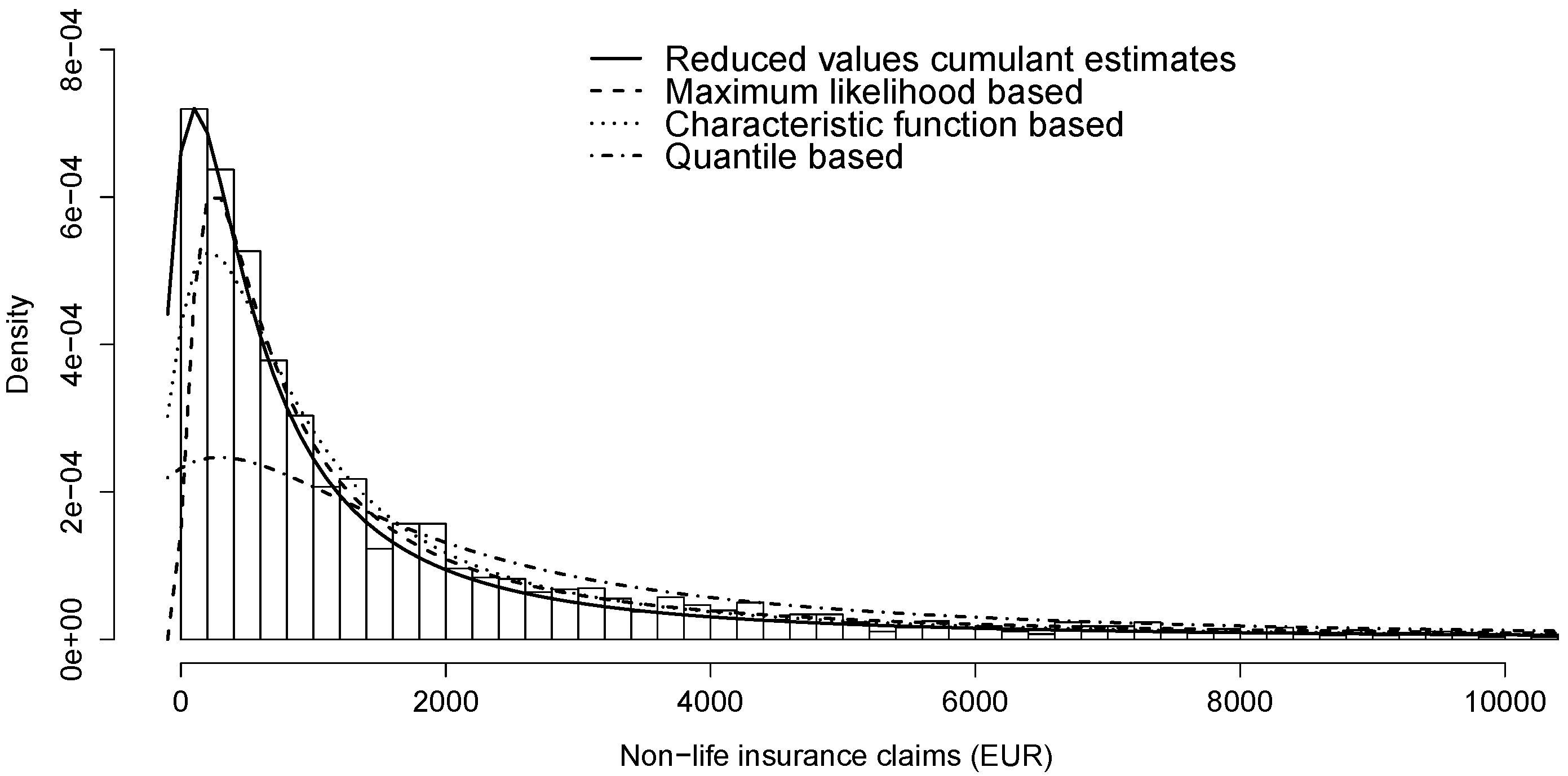
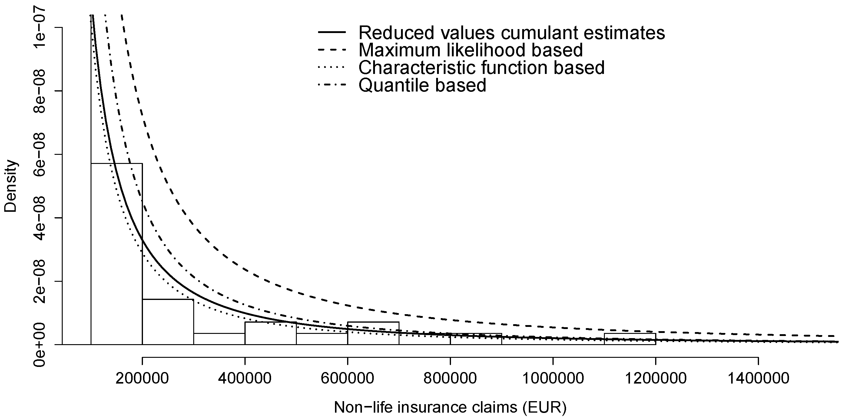
6.3. Comparison to Other Estimation Methods
7. Summary
- show that the parameters of stable law can be expressed through cumulant function of one pair of arguments, and hence
- propose the method of Press [6] at one pair of arguments only;
- suggest data scaling by median, i.e., introduce reduced values’ cumulant estimates;
- perform an empirical search for the selection of two arguments;
- carry out simulation experiments over parameter space at arguments of and ;
- present an application to non-life insurance losses;
Acknowledgments
Conflicts of Interest
Appendix A

| 0.03 | 0.03 | 0.03 | 0.03 | 0.3 | 0.3 | 0.3 | 0.3 | 3 | 3 | 3 | 3 | |
| 0.09 | 0.9 | 9 | 90 | 0.09 | 0.9 | 9 | 90 | 0.09 | 0.9 | 9 | 90 | |
| MSE () | 0.0000 | 0.0000 | 0.0059 | 0.0392 | 0.0000 | 0.0002 | 0.0163 | 0.0755 | 0.0007 | 0.0045 | 0.1520 | 0.2151 |
| MSE () | 0.0002 | 0.0001 | 0.0012 | 0.0091 | 0.0002 | 0.0007 | 0.0086 | 0.0311 | 0.0005 | 0.0231 | 4 × 101 | 3 × 101 |
| MSE () | 0.0001 | 0.0002 | 0.0425 | 0.3183 | 0.0001 | 0.0011 | 0.2077 | 7.7057 | 0.0002 | 0.1267 | Inf | Inf |
| MSE () | 0.0003 | 0.0000 | 0.0006 | 0.0000 | 0.0001 | 0.0002 | 0.0006 | 0.0000 | 0.0008 | 0.0030 | 0.0014 | 0.0000 |
| 0.03 | 0.03 | 0.03 | 0.03 | 0.3 | 0.3 | 0.3 | 0.3 | 3 | 3 | 3 | 3 | |
| 0.09 | 0.9 | 9 | 90 | 0.09 | 0.9 | 9 | 90 | 0.09 | 0.9 | 9 | 90 | |
| MSE () | 0.0001 | 0.0000 | 0.0000 | 0.0003 | 0.0000 | 0.0000 | 0.0000 | 0.0005 | 0.0000 | 0.0000 | 0.0001 | 0.0014 |
| MSE () | 0.0003 | 0.0001 | 0.0001 | 0.0043 | 0.0003 | 0.0002 | 0.0001 | 0.0146 | 0.0001 | 0.0002 | 0.0004 | 0.0993 |
| MSE () | 0.0036 | 0.0002 | 0.0002 | 0.0183 | 0.0012 | 0.0005 | 0.0002 | 0.0081 | 0.0001 | 0.0001 | 0.0003 | 0.0009 |
| MSE () | 0.0230 | 0.0006 | 0.0001 | 0.0218 | 0.0047 | 0.0013 | 0.0001 | 0.0235 | 0.0002 | 0.0004 | 0.0003 | 0.0318 |
| 0.03 | 0.03 | 0.03 | 0.03 | 0.3 | 0.3 | 0.3 | 0.3 | 3 | 3 | 3 | 3 | |
| 0.09 | 0.9 | 9 | 90 | 0.09 | 0.9 | 9 | 90 | 0.09 | 0.9 | 9 | 90 | |
| MSE () | 0.0001 | 0.3339 | 0.8957 | 1.2256 | 0.0933 | 2.2773 | 2.2475 | 2.2518 | 1.1632 | 2.2708 | 2.2755 | 2.2477 |
| MSE () | 0.0002 | 0.0414 | 0.0369 | 0.0594 | 0.2565 | 2 × 10² | 1 × 10² | 4 × 10² | 0.0653 | 2 × 10² | 2 × 10² | 4 × 10² |
| MSE () | 0.0000 | 0.1838 | 0.6175 | 0.8490 | 0.0056 | Inf | Inf | Inf | 1.0659 | Inf | Inf | Inf |
| MSE () | 0.0001 | 5 × 10³ | 0.0003 | 0.0000 | 8 × 101 | 0.1019 | 0.0004 | 0.0000 | 0.0029 | 0.0090 | 0.0010 | 0.0000 |
| 0.03 | 0.03 | 0.03 | 0.03 | 0.3 | 0.3 | 0.3 | 0.3 | 3 | 3 | 3 | 3 | |
| 0.09 | 0.9 | 9 | 90 | 0.09 | 0.9 | 9 | 90 | 0.09 | 0.9 | 9 | 90 | |
| MSE () | 0.0004 | 0.0001 | 0.1231 | 0.4640 | 0.0001 | 0.0000 | 0.3508 | 0.9181 | 0.0114 | 0.0928 | 2.2727 | 2.2629 |
| MSE () | 0.0011 | 0.0003 | 1.2741 | 1.9049 | 0.0002 | 0.0002 | 2.4033 | 4.4211 | 1.6320 | 5.1234 | 2 × 10² | 4 × 10² |
| MSE () | 0.0008 | 0.0000 | 0.3852 | 0.8615 | 0.0000 | 0.0000 | 0.1876 | 0.6170 | 0.0216 | 0.0039 | Inf | Inf |
| MSE () | 0.0003 | 0.0002 | 0.1416 | 0.0045 | 0.0002 | 0.0002 | 8.5030 | 0.0030 | 0.2452 | 5 × 101 | 0.0973 | 0.0005 |
Appendix B
| α | β | Method | MSE () | MSE () | MSE () | MSE () |
|---|---|---|---|---|---|---|
| 0.25 | 0.1 | RVCE | 5.7 × 10⁻⁶ | 6.9 × 10⁻⁵ | 1.5 × 10⁻⁴ | 1.7 × 10⁻⁶ |
| 0.25 | 0.1 | CE | 3.8 × 10⁻⁵ | 6.3 × 10⁻⁴ | 5.5 × 10⁻³ | 5.5 × 10⁻³ |
| 0.25 | 0.25 | RVCE | 4.1 × 10⁻⁶ | 4.9 × 10⁻⁵ | 6.6 × 10⁻⁵ | 1.4 × 10⁻⁵ |
| 0.25 | 0.25 | CE | 3.5 × 10⁻⁵ | 4.6 × 10⁻⁴ | 4.6 × 10⁻³ | 4.6 × 10⁻³ |
| 0.25 | 0.5 | RVCE | 4.3 × 10⁻⁶ | 5.2 × 10⁻⁵ | 3.8 × 10⁻⁴ | 1.7 × 10⁻⁴ |
| 0.25 | 0.5 | CE | 3.9 × 10⁻⁵ | 6.1 × 10⁻⁴ | 5.8 × 10⁻³ | 5.8 × 10⁻³ |
| 0.25 | 0.75 | RVCE | 3.4 × 10⁻⁶ | 5.9 × 10⁻⁵ | 5.8 × 10⁻⁴ | 8.9 × 10⁻⁴ |
| 0.25 | 0.75 | CE | 3.6 × 10⁻⁵ | 6.1 × 10⁻⁴ | 5.4 × 10⁻³ | 5.4 × 10⁻³ |
| 0.25 | 1 | RVCE | 4.2 × 10⁻⁶ | 1.0 × 10⁻⁴ | 1.1 × 10⁻³ | 4.3 × 10⁻³ |
| 0.25 | 1 | CE | 4.3 × 10⁻⁵ | 7.1 × 10⁻⁴ | 6.3 × 10⁻³ | 6.3 × 10⁻³ |
| 0.5 | 0.1 | RVCE | 4.1 × 10⁻⁶ | 1.8 × 10⁻⁵ | 1.5 × 10⁻⁵ | 3.0 × 10⁻⁵ |
| 0.5 | 0.1 | CE | 4.6 × 10⁻⁵ | 3.2 × 10⁻⁴ | 4.3 × 10⁻³ | 4.3 × 10⁻³ |
| 0.5 | 0.25 | RVCE | 3.7 × 10⁻⁶ | 2.5 × 10⁻⁵ | 5.5 × 10⁻⁵ | 1.2 × 10⁻⁴ |
| 0.5 | 0.25 | CE | 6.7 × 10⁻⁵ | 2.4 × 10⁻⁴ | 3.6 × 10⁻³ | 3.6 × 10⁻³ |
| 0.5 | 0.5 | RVCE | 5.5 × 10⁻⁶ | 2.4 × 10⁻⁵ | 1.5 × 10⁻⁴ | 3.2 × 10⁻⁴ |
| 0.5 | 0.5 | CE | 5.8 × 10⁻⁵ | 2.6 × 10⁻⁴ | 4.4 × 10⁻³ | 4.4 × 10⁻³ |
| 0.5 | 0.75 | RVCE | 7.4 × 10⁻⁶ | 3.6 × 10⁻⁵ | 2.9 × 10⁻⁴ | 1.1 × 10⁻³ |
| 0.5 | 0.75 | CE | 5.5 × 10⁻⁵ | 2.8 × 10⁻⁴ | 6.1 × 10⁻³ | 6.1 × 10⁻³ |
| 0.5 | 1 | RVCE | 8.5 × 10⁻⁶ | 3.9 × 10⁻⁵ | 4.5 × 10⁻⁴ | 2.5 × 10⁻³ |
| 0.5 | 1 | CE | 5.5 × 10⁻⁵ | 3.0 × 10⁻⁴ | 8.4 × 10⁻³ | 8.4 × 10⁻³ |
| 0.75 | 0.1 | RVCE | 4.5 × 10⁻⁶ | 1.6 × 10⁻⁵ | 2.0 × 10⁻⁵ | 1.9 × 10⁻⁴ |
| 0.75 | 0.1 | CE | 9.9 × 10⁻⁵ | 3.1 × 10⁻⁴ | 7.3 × 10⁻³ | 7.3 × 10⁻³ |
| 0.75 | 0.25 | RVCE | 8.3 × 10⁻⁶ | 2.5 × 10⁻⁵ | 8.8 × 10⁻⁵ | 6.7 × 10⁻⁴ |
| 0.75 | 0.25 | CE | 1.2 × 10⁻⁴ | 3.1 × 10⁻⁴ | 9.6 × 10⁻³ | 9.6 × 10⁻³ |
| 0.75 | 0.5 | RVCE | 1.2 × 10⁻⁵ | 3.9 × 10⁻⁵ | 2.0 × 10⁻⁴ | 2.5 × 10⁻³ |
| 0.75 | 0.5 | CE | 9.9 × 10⁻⁵ | 2.5 × 10⁻⁴ | 1.7 × 10⁻² | 1.7 × 10⁻² |
| 0.75 | 0.75 | RVCE | 2.0 × 10⁻⁵ | 4.0 × 10⁻⁵ | 4.2 × 10⁻⁴ | 8.3 × 10⁻³ |
| 0.75 | 0.75 | CE | 9.5 × 10⁻⁵ | 2.3 × 10⁻⁴ | 2.8 × 10⁻² | 2.8 × 10⁻² |
| 0.75 | 1 | RVCE | 2.1 × 10⁻⁵ | 5.4 × 10⁻⁵ | 5.3 × 10⁻⁴ | 1.6 × 10⁻² |
| 0.75 | 1 | CE | 9.4 × 10⁻⁵ | 2.3 × 10⁻⁴ | 4.3 × 10⁻² | 4.3 × 10⁻² |
| 0.1 | RVCE | 5.8 × 10⁻⁶ | 1.5 × 10⁻⁵ | 5.7 × 10⁻⁶ | 5.7 × 10⁻⁵ | |
| 0.1 | CE | 3.2 × 10⁻⁴ | 8.5 × 10⁻⁴ | 1.4 × 10⁻³ | 1.4 × 10⁻³ | |
| 0.25 | RVCE | 1.8 × 10⁻⁵ | 3.9 × 10⁻⁵ | 4.3 × 10⁻⁵ | 1.3 × 10⁻⁴ | |
| 0.25 | CE | 4.1 × 10⁻⁴ | 1.0 × 10⁻³ | 2.7 × 10⁻³ | 2.7 × 10⁻³ | |
| 0.5 | RVCE | 3.8 × 10⁻⁵ | 7.8 × 10⁻⁵ | 1.5 × 10⁻⁴ | 4.0 × 10⁻⁴ | |
| 0.5 | CE | 4.3 × 10⁻⁴ | 7.7 × 10⁻⁴ | 4.8 × 10⁻³ | 4.8 × 10⁻³ | |
| 0.75 | RVCE | 5.6 × 10⁻⁵ | 1.4 × 10⁻⁴ | 3.0 × 10⁻⁴ | 8.9 × 10⁻⁴ | |
| 0.75 | CE | 4.0 × 10⁻⁴ | 7.2 × 10⁻⁴ | 7.9 × 10⁻³ | 7.9 × 10⁻³ | |
| 1 | RVCE | 8.8 × 10⁻⁵ | 1.3 × 10⁻⁴ | 5.5 × 10⁻⁴ | 1.9 × 10⁻³ | |
| 1 | CE | 3.8 × 10⁻⁴ | 6.0 × 10⁻⁴ | 1.2 × 10⁻² | 1.2 × 10⁻² | |
| 0.1 | RVCE | 3.8 × 10⁻⁶ | 1.8 × 10⁻⁵ | 1.2 × 10⁻⁶ | 1.2 × 10⁻⁵ | |
| 0.1 | CE | 5.9 × 10⁻⁴ | 1.9 × 10⁻³ | 2.2 × 10⁻⁴ | 2.2 × 10⁻⁴ | |
| 0.25 | RVCE | 5.0 × 10⁻⁶ | 2.2 × 10⁻⁵ | 2.9 × 10⁻⁶ | 1.2 × 10⁻⁵ | |
| 0.25 | CE | 6.0 × 10⁻⁴ | 2.0 × 10⁻³ | 2.4 × 10⁻⁴ | 2.4 × 10⁻⁴ | |
| 0.5 | RVCE | 1.6 × 10⁻⁵ | 4.7 × 10⁻⁵ | 1.7 × 10⁻⁵ | 1.8 × 10⁻⁵ | |
| 0.5 | CE | 6.2 × 10⁻⁴ | 1.9 × 10⁻³ | 2.6 × 10⁻⁴ | 2.6 × 10⁻⁴ | |
| 0.75 | RVCE | 2.4 × 10⁻⁵ | 7.4 × 10⁻⁵ | 4.0 × 10⁻⁵ | 2.3 × 10⁻⁵ | |
| 0.75 | CE | 5.6 × 10⁻⁴ | 1.9 × 10⁻³ | 3.3 × 10⁻⁴ | 3.3 × 10⁻⁴ | |
| 1 | RVCE | 3.4 × 10⁻⁵ | 9.8 × 10⁻⁵ | 6.9 × 10⁻⁵ | 3.2 × 10⁻⁵ | |
| 1 | CE | 5.9 × 10⁻⁴ | 1.7 × 10⁻³ | 3.9 × 10⁻⁴ | 3.9 × 10⁻⁴ | |
| 0.1 | RVCE | 8.3 × 10⁻⁴ | 4.7 × 10⁻³ | 4.6 × 10⁻⁵ | 4.6 × 10⁻⁵ | |
| 0.1 | CE | 4.5 × 10⁻² | 4.6 × 10⁻¹ | 1.2 × 10⁻³ | 4.2 × 10⁻¹ | |
| 0.25 | RVCE | 4.0 × 10⁻⁶ | 6.3 × 10⁻⁵ | 1.2 × 10⁻⁶ | 6.3 × 10⁻⁶ | |
| 0.25 | CE | 8.0 × 10⁻⁴ | 6.1 × 10⁻³ | 7.1 × 10⁻⁵ | 7.1 × 10⁻⁵ | |
| 0.5 | RVCE | 3.0 × 10⁻⁶ | 3.1 × 10⁻⁵ | 1.0 × 10⁻⁶ | 4.2 × 10⁻⁶ | |
| 0.5 | CE | 7.8 × 10⁻⁴ | 7.1 × 10⁻³ | 6.5 × 10⁻⁵ | 6.5 × 10⁻⁵ | |
| 0.75 | RVCE | 5.7 × 10⁻⁶ | 4.4 × 10⁻⁵ | 2.0 × 10⁻⁶ | 4.6 × 10⁻⁶ | |
| 0.75 | CE | 7.6 × 10⁻⁴ | 7.4 × 10⁻³ | 5.8 × 10⁻⁵ | 5.8 × 10⁻⁵ | |
| 1 | RVCE | 8.1 × 10⁻⁶ | 9.1 × 10⁻⁵ | 3.4 × 10⁻⁶ | 5.2 × 10⁻⁶ | |
| 1 | CE | 9.7 × 10⁻⁴ | 9.4 × 10⁻³ | 7.3 × 10⁻⁵ | 7.3 × 10⁻⁵ |
References
- V.V. Uchaikin, and M.V. Zolotarev. Chance and Stability: Stable Distributions and Their Applications. Utrecht, The Netherland: Walter de Gruyter, 1999. [Google Scholar]
- I.A. Koutrouvelis. “Regression-type estimation of the parameters of stable laws.” J. Am. Stat. Assoc. 75 (1980): 918–928. [Google Scholar] [CrossRef]
- I.A. Koutrouvelis. “An iterative procedure for estimation of the parameters of stable laws.” Commun. Statist. Simul. Comput. 10 (1981): 17–28. [Google Scholar] [CrossRef]
- S.M. Kogon, and D.B. Williams. “Characteristic function based estimation of stable parameters.” In A Practical Guide to Heavy Tails. Edited by R. Adler, R. Feldman and M. Taqqu. Boston, MA, USA: Birkhäuser, 1998, pp. 311–335. [Google Scholar]
- A.S. Paulson, E.W. Holcomb, and R.A. Leitch. “The estimation of the parameters of the stable laws.” Biometrika 62 (1975): 163–170. [Google Scholar] [CrossRef]
- S.J. Press. “Estimation in univariate and multivariate stable distribution.” J. Am. Stat. Assoc. 67 (1972): 842–846. [Google Scholar] [CrossRef]
- Z. Fan. “Parameter Estimation of Stable Distributions.” Commun. Stat. Theory Methods 35 (2006): 245–255. [Google Scholar] [CrossRef]
- R. Höpfner, and L. Rüschendorf. “Comparison of estimators in stable models.” Math. Comput. Model. 29 (1999): 145–160. [Google Scholar] [CrossRef]
- G. Samorodnitsky, and M.S. Taqqu. Stable Non-Gaussian Random Processes: Stochastic Models with Infinite Variance. New York, NY, USA: Chapman and Hall/CRC, 1994. [Google Scholar]
- J.P. Nolan. Stable Distributions - Models for Heavy Tailed Data. Boston, MA, USA: Birkhäuser, 2016, Chapter 1; Available online: http://fs2.american.edu/jpnolan/www/stable/chap1.pdf (accessed on 23 September 2015).
- W. Feller. An introduction to Probability Theory and its Applications, 2nd ed. New York, NY, USA: Wiley, 1971, Volume 2. [Google Scholar]
- C. Heathcote. “The Integrated Squared Error Estimation of Parameters.” Biometrika 64 (1977): 255–264. [Google Scholar] [CrossRef]
- J. Yu. “Empirical Characteristic Function Estimation and Its Applications.” Econometr. Rev. 23 (2004): 93–123. [Google Scholar] [CrossRef]
- A.W. Van der Vaart. Asymptotic Statistics. New York, NY, USA: Cambridge University Press, 1998. [Google Scholar]
- J.L. Knight, and S.E. Satchell. “The Cumulant Generating Function Estimation Method.” Econometr. Theory 13 (1997): 170–184. [Google Scholar] [CrossRef]
- H.S. Kasana. Complex Variables: Theory And Applications, 2nd ed. New Delhi, India: Prentice-Hall of India Private Limited, 2005. [Google Scholar]
- E.F. Fama, and R. Roll. “Parameter estimates for symmetric stable distributions.” J. Am. Stat. Assoc. 66 (1978): 331–338. [Google Scholar] [CrossRef]
- D. Wuertz, and M. Maechler. Rmetrics Core Team Members Stabledist: Stable Distribution Functions, R Package Version 0.7-0; 2015. Available online: https://CRAN.R-project.org/package=stabledist (accessed on 20 January 2016).
- R Core Team. R: A language and environment for statistical computing. Vienna, Austria: R Foundation for Statistical Computing, 2015, Available online: http://www.R-project.org/ (accessed on 20 January 2016).
- S. Borak, K.W. Härdle, and R. Weron. “Stable Distributions.” In Statistical Tools for Finance and Insurance. Edited by P. Čižek, K.W. Härdle and R. Weron. Berlin, Germany: Springer, 2005, pp. 21–45. [Google Scholar]
- J.P. Nolan. “Maximum likelihood estimation and diagnostic for stable distributions.” In Lévy Processes. Edited by O.E. Barndorff-Nielsen, T. Mikosh and S. Resnick. Boston, MA, USA: Birkhäuser, 2001, pp. 379–400. [Google Scholar]
- J.H. McCullogh. “Simple consistent estimators of stable distributions parameters.” Commun. Stat. Simul. 15 (1986): 1109–1136. [Google Scholar] [CrossRef]
- J.P. Nolan. STABLE Program for Windows Version 3.14.02. 2005. Available online: http://academic2.american.edu/~jpnolan/stable/stable.html (accessed on 15 February 2016).
- S. Bates, and S. McLaughlin. “The estimation of stable distribution parameters.” In Proceedings of the IEEE Signal Processing Workshop on in Higher-Order Statistics; Chicago, IL, USA: IEEE Press, 1997, pp. 390–394. [Google Scholar]


| Argument | Values | |||||||||||
|---|---|---|---|---|---|---|---|---|---|---|---|---|
| 0.03 | 0.03 | 0.03 | 0.03 | 0.3 | 0.3 | 0.3 | 0.3 | 3 | 3 | 3 | 3 | |
| 0.09 | 0.9 | 9 | 90 | 0.09 | 0.9 | 9 | 90 | 0.09 | 0.9 | 9 | 90 | |
| Formula | (8) | (10) | (9) | (11) | |||
|---|---|---|---|---|---|---|---|
| MSE () | MSE () | MSE () | MSE () | MSE () | MSE () | ||
| 0.95 | 0.1 | 0.0000 | 0.0001 | 0.0003 | 0.0000 | 0.0458 | 1.6567 |
| 0.95 | 1 | 0.0003 | 0.0008 | 0.0688 | 0.0023 | 9 × 101 | 2 × 10² |
| 0.96 | 0.1 | 0.0000 | 0.0001 | 0.0002 | 0.0001 | 0.1537 | 2.6231 |
| 0.96 | 1 | 0.0005 | 0.0012 | 0.0496 | 0.0044 | 5 × 10⁴ | 3 × 10² |
| 0.98 | 0.1 | 0.0001 | 0.0002 | 0.0003 | 0.0003 | 7 × 101 | 1 × 101 |
| 0.98 | 1 | 0.0009 | 0.0027 | 0.0309 | 0.0135 | 4 × 10⁵ | 1 × 10³ |
| 0.99 | 0.1 | 0.0002 | 0.0005 | 0.0005 | 0.0007 | 1 × 10⁶ | 4 × 101 |
| 0.99 | 1 | 0.0017 | 0.0045 | 0.0553 | 0.0333 | 2 × 10⁴ | 4 × 10³ |
| 1.01 | 0.1 | 0.0002 | 0.0004 | 0.0004 | 0.0007 | 2 × 10⁵ | 4 × 101 |
| 1.01 | 1 | 0.0016 | 0.0060 | 0.0383 | 0.0278 | 4 × 10⁶ | 4 × 10³ |
| 1.02 | 0.1 | 0.0001 | 0.0002 | 0.0002 | 0.0002 | 1 × 10³ | 1 × 101 |
| 1.02 | 1 | 0.0009 | 0.0027 | 0.0202 | 0.0108 | 4 × 10⁴ | 9 × 10² |
| 1.04 | 0.1 | 0.0001 | 0.0001 | 0.0002 | 0.0001 | 0.1101 | 2.4367 |
| 1.04 | 1 | 0.0006 | 0.0015 | 0.0340 | 0.0046 | 2 × 10⁴ | 2 × 10² |
| 1.05 | 0.1 | 0.0000 | 0.0001 | 0.0001 | 0.0000 | 0.0458 | 1.5814 |
| 1.05 | 1 | 0.0005 | 0.0013 | 0.0392 | 0.0032 | 3 × 10² | 1 × 10² |
| Formula | (8) | (10) | (9) | (11) | ||
|---|---|---|---|---|---|---|
| MSE () | MSE () | MSE () | MSE () | MSE () | MSE () | |
| 0.1 | 0.0002 | 0.0004 | 0.0004 | 0.0013 | 5 × 101 | 0.0012 |
| 0.25 | 0.0002 | 0.0609 | 0.0609 | 0.0216 | 3 × 10³ | 0.0072 |
| 0.5 | 0.0002 | 0.2421 | 0.2422 | 0.0348 | 2 × 101 | 0.0430 |
| 0.75 | 0.0002 | 0.5476 | 0.5473 | 0.0443 | 1 × 10³ | 0.0938 |
| 1 | 0.0002 | 0.9717 | 0.9713 | 0.3854 | 5 × 10³ | 0.1925 |
| Min | 1st Quartile | Median | Mean | 3rd Quartile | Maximum |
|---|---|---|---|---|---|
| 15.3 | 358.0 | 955.0 | 6703.0 | 2781.0 | 1166000.0 |
| Mean () | Mean () | Mean () | Mean () | ||
|---|---|---|---|---|---|
| 0.03 | 0.09 | 0.13 | 1.62 | 9 × 1077 | –3.77 |
| 0.03 | 0.9 | 0.01 | 6.70 | Inf | 1.53 |
| 0.03 | 9 | 0.03 | 2.98 | Inf | –0.10 |
| 0.03 | 90 | 0.02 | –0.76 | Inf | –0.02 |
| 0.3 | 0.09 | 0.04 | –0.42 | Inf | 3.05 |
| 0.3 | 0.9 | –0.17 | –1.22 | Inf | 1.93 |
| 0.3 | 9 | –0.01 | –1.46 | Inf | –0.17 |
| 0.3 | 90 | –0.01 | 0.79 | Inf | –0.02 |
| 3 | 0.09 | 0.01 | –2.35 | Inf | 0.12 |
| 3 | 0.9 | 0.14 | 2.18 | 3 × 10125 | –0.87 |
| 3 | 9 | –0.04 | 0.36 | 5× 10184 | –0.29 |
| 3 | 90 | –0.03 | 0.59 | Inf | –0.02 |
| Mean | CV | Mean | CV | Mean | CV | Mean | CV | ||
|---|---|---|---|---|---|---|---|---|---|
| () | () | () | () | () | () | () | () | ||
| 0.03 | 9 | 0.71 | 0.030 | 1.19 | 0.059 | 382.46 | 0.073 | –432.25 | 0.206 |
| 3 | 0.09 | 0.72 | 0.030 | 1.12 | 0.042 | 444.48 | 0.045 | –574.15 | 0.209 |
| 0.3 | 9 | 0.67 | 0.032 | 1.17 | 0.046 | 410.33 | 0.059 | –335.48 | 0.181 |
| 0.03 | 0.9 | 0.77 | 0.039 | 1.05 | 0.057 | 568.07 | 0.057 | –1113.55 | 0.328 |
| 0.03 | 90 | 0.56 | 0.039 | 1.78 | 0.079 | 119.88 | 0.192 | –103.29 | 0.181 |
| 0.3 | 0.9 | 0.80 | 0.048 | 1.06 | 0.055 | 578.91 | 0.059 | –1460.33 | 0.342 |
| 0.3 | 90 | 0.48 | 0.058 | 1.87 | 0.085 | 181.45 | 0.175 | –85.05 | 0.183 |
| 3 | 0.9 | 0.60 | 0.064 | 1.18 | 0.061 | 475.25 | 0.046 | –283.09 | 0.345 |
| 0.3 | 0.09 | 0.75 | 0.069 | 1.00 | 0.072 | 523.66 | 0.145 | –819.13 | 0.793 |
| 0.03 | 0.09 | 0.78 | 0.099 | 1.09 | 0.101 | 581.48 | 0.304 | –1989.91 | 1.272 |
| 3 | 9 | 0.60 | 0.107 | 0.94 | 0.133 | 484.41 | 0.092 | –139.00 | 0.608 |
| 3 | 90 | 0.33 | 0.151 | 2.00 | 0.157 | 690.79 | 0.194 | –60.62 | 0.204 |
© 2016 by the author; licensee MDPI, Basel, Switzerland. This article is an open access article distributed under the terms and conditions of the Creative Commons Attribution (CC-BY) license (http://creativecommons.org/licenses/by/4.0/).
Share and Cite
Krutto, A. Parameter Estimation in Stable Law. Risks 2016, 4, 43. https://doi.org/10.3390/risks4040043
Krutto A. Parameter Estimation in Stable Law. Risks. 2016; 4(4):43. https://doi.org/10.3390/risks4040043
Chicago/Turabian StyleKrutto, Annika. 2016. "Parameter Estimation in Stable Law" Risks 4, no. 4: 43. https://doi.org/10.3390/risks4040043
APA StyleKrutto, A. (2016). Parameter Estimation in Stable Law. Risks, 4(4), 43. https://doi.org/10.3390/risks4040043