Analysis of Insurance Claim Settlement Process with Markovian Arrival Processes

Abstract

This paper proposes a model for the claim occurrence, reporting, and handling process of insurance companies. It is assumed that insurance claims occur according to a Markovian arrival process. An incurred claim goes through some stages of a claim reporting and handling process, such as Incurred But Not Reported (IBNR), Reported But Not Settled (RBNS) and Settled (S). We derive formulas for the joint distribution and the joint moments for the amount of INBR, RBNS and Settled claims. This model generalizes previous ones in the literature, which generally assume Poisson claim arrivals. Due to the flexibility of the Markovian arrival process, the model can be used to evaluate how the claim occurring, reporting, and handling mechanisms may affect the volatilities of the amount of IBNR, RBNS and Settled claims, and the interdependencies among them.

1. Introduction

In property and casualty insurance, the loss payment delay related to claim reporting and handling can be significant. For example, an injury may not be reported by the victim until years after the accident or exposure that caused it, especially for latent diseases. Reported claims often remain unpaid for long periods, since court backlogs, discovery procedures, and legal negotiations delay settlement. Therefore, it is customary to categorize incurred claims into Incurred But Not Reported (IBNR), Reported But Not Settled (RBNS), and Settled (S), etc.

Insurers can only observe claims that have been reported, yet they are required to reserve funds for all incurred claims. Therefore, methods to estimate the distribution of incurred losses based on the insurer’s information about paid and/or reported amount have been studied extensively in the actuarial literature. For example, Arjas (1989) [1] laid out a structure for modelling the claim reporting/handling process as a marked point process, where each incurred claim (point) is associated with a random mark that carries information about how it is categorized into different stages of settlement over time. The author showed how to use martingale theory to estimate IBNR claims based on information included in reported claims. Norberg (1993) [2] assumed that claims occur according to a time–inhomogeneous Poisson process and that the time from claim occurrence to reporting and time from claim reporting to settlement follow arbitrary distributions. It was showed that the IBNR, RBNS, and Settled (S) claims all follow compound Poisson distributions and that they are independent. For a more recent treatment, one is referred to Chapter 8 of Mikosch (2009) [3].

Instead of assuming certain probability distributions for the claim reporting/handling delays, the claim reporting/handling process may be represented by a Markov chain. This idea was proposed in Hachemeister (1980) [4], and was followed by, for example, Hesselager (1994) [5], who assumed that the claims arrive according to a Poisson process and derived the moments of the IBNR and RBNS claims.

As was pointed out in Hesselager (1994) [5] and Norberg (1993) [2], when it is assumed that the claims occur according to a Poisson process, due to the properties of marked Poisson processes, the amount of claims in different settlement stages (such as IBNR, RBNS) are independent - a statement that has not been tested empirically. The purpose of the current paper is not to argue whether the assumption of independencies among the claims in different stages of the settlement process is reasonable or not. Instead, we propose a general model that allows interdependencies among claims in difference stages of the settlement process. As argued in Neuhaus (2004) [6], since claim development between two valuation dates comprises two separate types of development: changes in the assessment of reported incurred claims, and reports of new claims that are received by the insurer, it could be advantageous to distinct between the cost of reported claims and the cost of unreported claims in claim reserving. Information on their dependency will be important when aggregating both costs to estimate the variation of the total claim development.

Specifically, we assume that claims occur according to a Markovian arrival process (MAP) (see for example, Asmussen 2003 [7]), and that an incurred claim goes through some stages of a claim reporting/handling process according to a Markovian law. We derive formulas for the joint distribution and the joint moments for the amount of INBR, RBNS and Settled claims. Since the MAP is quite general and includes Poisson processes, renewal processes with phase–type inter–arrival times and Markov modulated Poisson processes as special cases, our model may be used to evaluate how different claim occurring/handling processes may affect the volatility of the IBNR, RBNS, and Settled claims and their interdependencies. As an example, in Section 5, we assume that the claim occurrence frequency is influenced by an external environment, which evolves according to a Markov chain, so the claims arrive according to a Markov modulated Poisson process. Using the results developed in Section 3 and 4, we show that in this case the amount of IBNR and RBNS claims are more volatile than in the case when claims arrive according to a homogeneous Poisson process. In addition, the amount of IBNR and RBNS claims are stochastically dependent.

Methodologically, we will follow Willmot (1990) [8], which recognized the connections between the distribution of the number of IBNR claims and the number of customers in an infinite server queue, where the service time of the queue is analogous to the time needed to report a claim. This allows us to make use of the results on the distribution of the number of customers in an infinite server queue with Markovian arrivals in the queueing literatures (see for example, Ramaswami and Neuts 1980 [9] and Masuyama and Takine 2002 [10]).

The remaining parts of this paper are organized as follows. Section 2 introduces the claim occurrence and settlement processes; Section 3 derives an equation that characterizes the joint distribution of the amount of the claims in different stages of the settlement process; Section 4 derives formulas for the joint moments; Section 5 presents numerical examples; Section 6 concludes.

2. The Model

2.1. The Claim Incurral Process

We assume that claims occur according to a MAP with representation $\left(\gamma ,{\mathbf{D}}_0,{\mathbf{D}}_1\right)$. That is, let $J\left(t\right)$ be an irreducible continuous time Markov process with $m<\infty$ states, initial distribution γ, intensity matrix $\mathbf{D}={\left(D_{i,j}\right)}_{i,j\in 1,2,\cdots ,m}$, and limiting distribution π. A transition in $J\left(t\right)$ may be accompanied by the occurrence of a claim. As such, the intensity matrix $\mathbf{D}$ has the decomposition $\mathbf{D}={\mathbf{D}}_0+{\mathbf{D}}_1$, where ${\mathbf{D}}_0$ is the matrix of intensities of state changes without arrivals and ${\mathbf{D}}_1$ that of state changes with arrivals. Claims that arrive with the $i\to j$ transitions are assumed to have probability distribution function $F_{ij}$, density function $f_{ij}$, kth moments ${\mu }_{ij}^{\left(k\right)}$ and moment generating function (mgf) $f_{ij}^{*}\left(s\right)={\int }_0^{\infty }{e}^{sx}{f}_{ij}\left(x\right)dx$. In addition, we let ${\mathbf{D}}_f\left(x\right)$ denote a matrix with the $ij$th element ${\left\{{\mathbf{D}}_f\left(x\right)\right\}}_{ij}={\left\{{\mathbf{D}}_1\right\}}_{ij}{f}_{ij}\left(x\right);$ for $k\ge 1,$ let ${\mathbf{D}}_{\mu ,k}$ be a matrix with the $ij$th element ${\left\{{\mathbf{D}}_{\mu ,k}\right\}}_{ij}={\left\{{\mathbf{D}}_1\right\}}_{ij}{\mu }_{ij}^{\left(k\right)}$, let ${\mathbf{D}}_f^{*}\left(s\right)$ be a matrix with the $ij$th element ${\{{\mathbf{D}}_f^{*}\left(s\right)\}}_{ij}={\left\{{\mathbf{D}}_1\right\}}_{ij}{f}_{ij}^{*}\left(s\right)$ for $1\le i,j\le m.$

2.2. The Claim Reporting and Handling Process

As in Hesselager (1994) [5], the claim reporting and handling process is modelled by a continuous time Markov chain $I\left(t\right)$ with state space $S=\{0,1,\cdots ,K\}$. Let $S=S_{IBNR}\cup S_{RBNS}\cup S_S$, where $S_{IBNR}=\{1,\cdots ,K_1\}$, $S_{RBNS}=\{K_1+1,\cdots ,K\}$, and $S_S=\left\{0\right\}$ denote subsets containing IBNR, RBNS and Settled states respectively. The state 0 is assumed to be absorbing, which means that there is no further development after a claim is settled.

An incurred claim is initially assigned to a state j in the set of transient states $\{1,\cdots ,K\}$ with probability ${\beta }_j$. The matrix of the rates of transitions among the transient states is denoted by $\mathbf{T}$ and the vector of rates of transitions from transient states to the absorbing state is denoted by $\mathbf{t}$. Then, the total time a claim spends in the claim reporting and handling process follows a phase–type distribution with representation $(\beta ,\mathbf{T})$, where $\beta ={\left\{{\beta }_j\right\}}_{j=1,\cdots ,K}$.

In fact, the model structure requires that both the claim reporting and the claim handling time follow phase type distributions. Since it is well–known that the family of phase–type distributions is dense in the set of all positive-valued distributions (Asmussen 2003) [7], the current model can be used to approximate other models that directly assume certain claim reporting/handling delay distributions.

In addition, the proposed model is quite flexible in that one can add more states into the state space S to represent additional features of the claim reporting/handling process. For example, in insurance practice, a settled claim can be reopened. Reopened claims can be included in the model, for example, by introducing a state “pre-settled” in the subset $S_{RBNS}$, where a claim in the “pre-settled” state can move to the state 0 (Settled) with certain probability, but it also may move back to some other state in $S_{RBNS}$, representing a reopened claim.

3. The Joint Distribution of Claims in Different States

Let $\mathbf{X}\left(t\right)=\left(X_0\left(t\right),X_1\left(t\right),\cdots ,X_K\left(t\right)\right)$, $t\ge 0$, denote the amount of claims incurred during time interval $(0,t]$ and is at stage $\{0,1,\cdots ,K\}$ of claim reporting/handling process. Let $\mathbf{G}(\mathbf{x},t)$ be a matrix of conditional probabilities with the $ij$th element

$$G_{ij}(\mathbf{x},t)=\mathbb{P}\left[\mathbf{X}\left(t\right)\le \mathbf{x},J\left(t\right)=j\left|J\right(0)=i\right],i,j=1,2,\cdots ,m.$$

(1)

Let

$${\mathbf{G}}^{*}(\xi ,t)=\int e^{\xi ·\mathbf{x}\left(t\right)}d\mathbf{G}(\mathbf{x},t),$$

where $\xi =\{{\xi }_0,{\xi }_1,\cdots ,{\xi }_K\}$, be the moment generating function (mgf) of $\mathbf{G}(\mathbf{x},t).$

For $i\ge 1$, let $T_i$ and $Y_i$ denote the time of occurrence and the size of the ith claim respectively. Then we have that

$$\begin{array}{c}\hfill \mathbb{E}\left[e^{\xi ·\mathbf{x}\left(t\right)}1(T_1>t,J\left(t\right)=j)|J\left(0\right)=i\right]={\left\{e^{{\mathbf{D}}_{0}t}\right\}}_{ij},\end{array}$$

(2)

where $1(·)$ denotes an indicator function, which takes value 1 if the argument(s) is true and 0 otherwise.

For $n\ge 1$

$$\begin{array}{c}\mathbb{E}\left[e^{\xi ·\mathbf{X}\left(t\right)}|N\left(t\right)=n,\mathrm{and}\mathrm{for}i=1,\cdots n,T_i=t_i,Y_i=y_i\right]\hfill \\ =\prod _{i=1}^n\left(\sum _{k=0}^K{p}_k(t-t_i)e^{{\xi }_k{y}_i}\right),\hfill \end{array}$$

(3)

where for $k=0,1,\cdots ,K$, $p_k(t-t_i)$ is the probability that a claim that occurs at time $t_i$ is at stage k of the claim reporting/handling process at time t. Because of the assumed Markovian structure of the claim reporting/handling process, for $k=1,\cdots ,K$, $p_k(t-t_i)$=$\beta e^{\mathbf{T}(t-t_i)}{\mathbf{e}}_k$, where ${\mathbf{e}}_k$ denotes the kth column of an identity matrix, and $p_0(t-t_i)=1-{\sum }_{k=1}^K{p}_k(t-t_i)$.

It follows by using the law of total probability that

$$\begin{array}{c}\mathbb{E}\left[e^{\xi ·\mathbf{X}\left(t\right)}1(T_1<t,J\left(t\right)=j)|J\left(0\right)=i\right]\hfill \\ =\sum _{n=1}^{\infty }{\int }_0^{t}d{t}_1{\int }_{t_1}^{t}d{t}_2\cdots {\int }_{t_{n-1}}^{t}d{t}_n{\int }_0^{\infty }d{y}_1\cdots {\int }_0^{\infty }d{y}_n\hfill \\ {\left\{\prod _{i=1}^n\left[e^{{\mathbf{D}}_0(t_i-t_{i-1})}{\mathbf{D}}_f\left(y_i\right)\left(\sum _{k=0}^K{p}_k(t-t_i)e^{{\xi }_k{y}_i}\right)\right]e^{{\mathbf{D}}_0(t-t_n)}\right\}}_{ij}\hfill \\ =\sum _{n=1}^{\infty }{\int }_0^{t}d{t}_1{\int }_{t_1}^{t}d{t}_2\cdots {\int }_{t_{n-1}}^{t}d{t}_n\hfill \\ {\left\{\prod _{i=1}^n\left[e^{{\mathbf{D}}_0(t_i-t_{i-1})}{\mathbf{D}}_1^{*}(\xi ,t-t_i)\right]e^{{\mathbf{D}}_0(t-t_n)}\right\}}_{ij},\hfill \end{array}$$

(4)

where

$${\mathbf{D}}_1^{*}(\xi ,t-t_i)=\sum _{k=0}^K{p}_k(t-t_i){\mathbf{D}}_f^{*}\left({\xi }_k\right).$$

(5)

Combining Equations (2) and (4), we have

$$\begin{array}{c}\hfill {\mathbf{G}}^{*}(\xi ,t)=\left\{e^{{\mathbf{D}}_{0}t}\right\}+\sum _{n=1}^{\infty }{\int }_0^{t}d{t}_1{\int }_{t_1}^{t}d{t}_2\cdots {\int }_{t_{n-1}}^{t}d{t}_n\prod _{i=1}^n\left[e^{{\mathbf{D}}_0(t_i-t_{i-1})}{\mathbf{D}}_1^{*}(\xi ,t-t_i)\right]e^{{\mathbf{D}}_0(t-t_n)}\end{array}$$

(6)

Using similar arguments as in the derivation of Theorem 3.1 in Masuyama and Takine (2002) [10], Equation (6) leads to

Theorem 1. 

$$\begin{array}{c}\hfill \frac{\partial }{\partial t}{\mathbf{G}}^{*}(\xi ,t)=\left[{\mathbf{D}}_0+{\mathbf{D}}_1^{*}(\xi ,t)\right]{\mathbf{G}}^{*}(\xi ,t),\end{array}$$

(7)

where

$$\begin{array}{c}\hfill {\mathbf{D}}_1^{*}(\xi ,t)=\sum _{k=0}^K{p}_k\left(t\right){\mathbf{D}}_f^{*}\left({\xi }_k\right).\end{array}$$

(8)

The proof of the Theorem is provided in the appendix of the current paper.

Remark 1. It can be seen from Equation (7) that

$$\begin{array}{c}\hfill \frac{\partial }{\partial t}\mathbf{G}(\mathbf{x},t)={\mathbf{D}}_0\mathbf{G}(\mathbf{x},t)+\sum _{k=0}^K{p}_k\left(t\right){\int }_0^{x_k}{\mathbf{D}}_f\left(y\right)\mathbf{G}(\mathbf{x}-y{\mathbf{e}}_k,t)dy,\end{array}$$

(9)

where $x_k$ is the kth element of $\mathbf{x}$ and ${\mathbf{e}}_k$ is the kth column vector of a $(K+1)\times (K+1)$ identity matrix.

Intuitively, considering what may occur during a small time interval $(0,h)$, we have

$$\begin{array}{cc}{G}_{ij}(\mathbf{x},t)\hfill & =\sum _{l=1}^{m}h\left[\sum _{k=0}^K{p}_k\left(t\right){\int }_0^{x_j}{\left\{{\mathbf{D}}_{1f}\left(y\right)\right\}}_{il}{G}_{lj}(\mathbf{x}-y{\mathbf{e}}_k,t-h)dy\right]\hfill \\ & +\sum _{\begin{array}{c}1\le l\le m\\ l\ne i\end{array}}h{\left\{{\mathbf{D}}_0\right\}}_{il}{G}_{lj}(\mathbf{x},t-h)\hfill \\ & +(1+{\left\{{\mathbf{D}}_0\right\}}_{ii}h)G_{ij}(\mathbf{x},t-h).\hfill \end{array}$$

(10)

Letting $h\to 0$ yields Equation (9).

4. The Joint Moments

For $k=0,\cdots ,K$ and $l\ge 1$, let

$${\left\{{\mathbf{m}}_k^l\left(t\right)\right\}}_i=\mathbb{E}\left[{\left[X_k\left(t\right)\right]}^l|J\left(0\right)=i\right],i=1,\cdots ,m,$$

be the lth moment of $X_k\left(t\right)$ conditional on $J\left(0\right)=i$. Let ${\mathbf{m}}_k^l\left(t\right)$ denote the vector of conditional moments with the ith element being ${\left\{{\mathbf{m}}_k^l\left(t\right)\right\}}_i$. Let ${\mathbf{m}}_k\left(t\right)$ denote ${\mathbf{m}}_k^1\left(t\right)$.

Then, differentiating both sides of Equation (7) with respect to ${\xi }_k$ and rearranging, we obtain for $k=0,1,\cdots ,K$

$$\frac{d}{dt}{\mathbf{m}}_k^l\left(t\right)=\mathbf{D}{\mathbf{m}}_k^l\left(t\right)+p_k\left(t\right)\sum _{i=1}^l\left(\begin{array}{c}l\\ i\end{array}\right){\mathbf{D}}_{\mu ,i}{\mathbf{m}}_k^{l-i}\left(t\right),$$

(11)

where

$${\mathbf{m}}_k^0\left(t\right)=e^{Dt}\mathbf{e}=\mathbf{e}$$

and ${\mathbf{D}}_{\mu ,i}$ is a matrix with $ab$th element ${\left\{{\mathbf{D}}_1\right\}}_{ab}\times {\mu }_{ab}^{\left(i\right)}$ for $1\le a,b\le m$.

In particular,

$$\frac{d}{dt}{\mathbf{m}}_k\left(t\right)=\mathbf{D}{\mathbf{m}}_k\left(t\right)+p_k\left(t\right){\mathbf{D}}_{\mu ,1}\mathbf{e},$$

(12)

which has the solution

$${\mathbf{m}}_k\left(t\right)=e^{\mathbf{D}t}{\int }_0^t{p}_k\left(s\right)e^{-\mathbf{D}s}{\mathbf{D}}_{\mu ,1}\mathbf{e}ds.$$

(13)

For $k_1,k_2=0,1,\cdots ,K$, $k_1\ne k_2$, and $l_1,l_2\ge 0$, let ${\mathbf{m}}_{k_1,k_2}^{l_1,l_2}\left(t\right)$ be a vector having the ith element

$${\{{\mathbf{m}}_{k_1,k_2}^{l_1,l_2}\left(t\right)\}}_i=\mathbb{E}\left[\left[X_{k_1}^{l_1}\left(t\right)X_{k_2}^{l_2}\left(t\right)\right]|J\left(0\right)=i\right],i=1,\cdots ,m.$$

Then by differentiating both sides of Equation (7), we have

$$\frac{d}{dt}{\mathbf{m}}_{k_1,k_2}^{(l_1,l_2)}\left(t\right)=\mathbf{D}{\mathbf{m}}_{k_1,k_2}^{l_1,l_2}\left(t\right)+\sum _{(i,j)>0}^{l_1,l_2}\left(\begin{array}{c}{l}_1\\ i\end{array}\right)\left(\begin{array}{c}{l}_2\\ j\end{array}\right){\mathbf{D}}_{\mu ,k_1,k_2}^{i,j}{\mathbf{m}}_{k_1,k_2}^{l_1-i,l_2-j}\left(t\right),$$

(14)

where ${\mathbf{D}}_{\mu ,k_1,k_2}^{i,j}=\frac{{\partial }^{i+j}{\mathbf{D}}_1^{*}(\xi ,t)}{\partial {\xi }_{k_1}^i\partial {\xi }_{k_2}^j}{|}_{{\xi }_0,{\xi }_1,\cdots ,{\xi }_K=0}$.

Noticing that by Equation (8),

$${\mathbf{D}}_{\mu ,k_1,k_2}^{i,j}=\left\{\begin{array}{cc}0& \mathrm{if}\mathrm{i}>0\mathrm{and}\mathrm{j}>0\\ p_{k_1}\left(t\right){\mathbf{D}}_{\mu ,i}& \mathrm{if}\mathrm{i}>0\mathrm{and}\mathrm{j}=0\\ p_{k_2}\left(t\right){\mathbf{D}}_{\mu ,j}& \mathrm{if}\mathrm{i}=0\mathrm{and}\mathrm{j}>0\end{array}\right..$$

So Equation (14) can be simplified to

$$\begin{array}{cc}\frac{d}{dt}{\mathbf{m}}_{k_1,k_2}^{l_1,l_2}\left(t\right)=\mathbf{D}{\mathbf{m}}_{k_1,k_2}^{l_1,l_2}\left(t\right)\hfill & +{\sum }_{i=1}^{l_1}\left(\begin{array}{c}{l}_1\\ i\end{array}\right)p_{k_1}\left(t\right){\mathbf{D}}_{\mu ,i}{\mathbf{m}}_{k_1,k_2}^{l_1-i,l_2}\left(t\right)\hfill \\ & +{\sum }_{j=1}^{l_2}\left(\begin{array}{c}{l}_2\\ j\end{array}\right)p_{k_2}\left(t\right){\mathbf{D}}_{\mu ,j}{\mathbf{m}}_{k_1,k_2}^{l_1,l_2-j}\left(t\right).\hfill \end{array}$$

(15)

In particular, let ${\mathbf{m}}_{k_1,k_2}\left(t\right)$ denote ${\mathbf{m}}_{k_1,k_2}^{1,1}\left(t\right)$, then it satisfies

$$\frac{d}{dt}{\mathbf{m}}_{k_1,k_2}\left(t\right)=\mathbf{D}{\mathbf{m}}_{k_1,k_2}\left(t\right)+p_{k_1}\left(t\right){\mathbf{D}}_{\mu ,1}{\mathbf{m}}_{k_2}\left(t\right)+p_{k_2}\left(t\right){\mathbf{D}}_{\mu ,1}{\mathbf{m}}_{k_1}\left(t\right).$$

(16)

Remark 2. Let ${\left\{{\mathbf{m}}_{IBNR}^l\left(t\right)\right\}}_i$ be the lth moment of the amount of IBNR claims conditional on $J\left(0\right)=i$. Since $S_{IBNR}=\{1,\cdots ,K_1\}$, we have

$${\left\{{\mathbf{m}}_{IBNR}^l\left(t\right)\right\}}_i=\mathbf{E}\left[{\left(\sum _{k=1}^{K_1}{X}_k\left(t\right)\right)}^l|J\left(0\right)=i\right].$$

This can be calculated by making use of formula (15).

The unconditional moments of $\mathbf{X}\left(t\right)$ are obtained by pre–multiplying the vector of conditional moments by the initial distribution γ of the claim arrival process. When the claim arrival process is stationary, i.e., $\gamma =\pi$, the calculation of the unconditional moments simplifies because $\pi \mathbf{D}=\mathbf{0}$ and if we pre–multiply the moment formulas (11) and (15) by π, the first term on right hand side of the equations becomes zero. Particularly, for the first moments, we have that

$$\frac{d}{dt}\pi {\mathbf{m}}_k\left(t\right)=p_k\left(t\right)\pi {\mathbf{D}}_{\mu ,1}\mathbf{e},$$

(17)

which gives the simple formulas

$$\begin{array}{cc}\pi {\mathbf{m}}_k\left(t\right)\hfill & ={\int }_0^t{p}_k\left(\tau \right)d\tau \pi {\mathbf{D}}_{\mu ,1}\mathbf{e}\hfill \\ & ={\int }_0^t\beta e^{\mathbf{T}\tau }{\mathbf{e}}_{k}d\tau \pi {\mathbf{D}}_{\mu ,1}\mathbf{e}\hfill \\ & =\beta {\mathbf{T}}^{-1}(e^{\mathbf{T}t}-\mathbf{I}){\mathbf{e}}_k\pi {\mathbf{D}}_{\mu ,1}\mathbf{e},\mathrm{for}k=1,\cdots ,K,\hfill \end{array}$$

(18)

and

$$\pi {\mathbf{m}}_0\left(t\right)=\left(t-\beta {\mathbf{T}}^{-1}(e^{\mathbf{T}t}-\mathbf{I})\mathbf{e}\right)\pi {\mathbf{D}}_{\mu ,1}\mathbf{e}.$$

When $t\to \infty$, we have for $k=1,\cdots ,K,$

$$\begin{array}{c}\hfill \pi {\mathbf{m}}_k\left(t\right)\to (-\beta {\mathbf{T}}^{-1}{\mathbf{e}}_k)\left(\pi {\mathbf{D}}_{\mu ,1}\mathbf{e}\right),\end{array}$$

(19)

where the term $-\beta {\mathbf{T}}^{-1}{\mathbf{e}}_k$ is in fact the expected amount of time a claim stays in stage k before settlement (absorption).

Remark 3. Let ${\mathbf{m}}^l\left(t\right)$ denote the vector of conditional moments of the total amount of incurred claims during $(0,t]$, regardless of the claim reporing/handling status. Then it can be calculated by setting $p_k\left(t\right)=1$ in equation (11). In the equilibrium case, we have that $\pi \mathbf{m}\left(t\right)=\pi {\mathbf{D}}_{\mu ,1}\mathbf{e}t.$ This result will be used in the next section.

Remark 4. Similar to Section 8 of Ramaswami and Neuts (1980) [9], it can be shown that when $t\to \infty$, the distribution of ${\mathbf{X}}_k\left(t\right),k\in \{S_{IBNR}\cup S_{RBNS}\}$ has an asymptotical limit and the joint moments ${\mathbf{m}}_{k_1,k_2}^{l_1,l_2}\left(t\right)$ for $k_1,k_2\in \{S_{IBNR}\cup S_{RBNS}\}$ converges to a finite vector. This fact is actually illustrated in the numerical examples in the next section.

Remark 5. Since the calculation of the joint moments of $\mathbf{X}\left(t\right)$ only requires the moments of the claim sizes – the exact form of the claim size distribution is not needed. In the following numerical examples, exponential claim sizes are assumed for presentational convenience only.

5. Numerical Examples

This example considers three cases of the claim arrival process and illustrates how they affect the moments of the amount of IBNR and RBNS claims and their dependency. In the following, a random variable following an exponential distribution with rate λ is said to follow an $Exp\left(\lambda \right)$ distribution.

Case 1: Claims arrive according to a Poisson process with inter claim arrival times following an $Exp\left(140\right)$ distribution. The claim sizes follow an $Exp(140/190)$ distribution. In terms of the MAP representation, we have

$$\gamma =1,{\mathbf{D}}_0=-140\mathrm{and}{\mathbf{D}}_1=140.$$

Case 2: The claims arrive according to a Markov modulated Poisson process and claim sizes are modulated by the states of the underlying Markov process. Specifically, assume that an external environment evolves according to a continuous time Markov chain ${\left\{E\left(t\right)\right\}}_{t\ge 0}$ with a state space $\{N,R\}$, where the two elements standing for normal and risky environment respectively. The environment process is assumed to have the infinitesimal generator

$$Q=\left(\begin{array}{cc}-{\sigma }_1& {\sigma }_1\\ {\sigma }_2& -{\sigma }_2\end{array}\right),$$

where ${\sigma }_1=1$ and ${\sigma }_2=9$. The equilibrium distribution of the environment states is given by $\pi =[0.9,0.1],$ which means that in the long run, with $90\%$ chance, the environment is normal and with $10\%$ chance the environment is risky. In the normal environment N, the claim occurrence rate is ${\lambda }_N=100$ and the claim sizes follow an $Exp\left(1\right)$ distribution. In the risky environment R, the claim occurrence rate is ${\lambda }_R=500$ and the claim sizes follow an $Exp(1/2)$ distribution.

Assuming that the claim arrival process is stationary, the MAP representation is given by

$$\gamma =\pi =[0.9,0.1],{\mathbf{D}}_0=\left[\begin{array}{cc}-101& 1\\ 9& -509\end{array}\right]\mathrm{and}{\mathbf{D}}_1=\left[\begin{array}{cc}100& 0\\ 0& 500\end{array}\right].$$

Case 3: This case is similar to Case 2, but with different parameter values. Here it is assumed that the environment process has state space $\{N,R\}$ and have the infinitesimal generator

$$Q=\left(\begin{array}{cc}-{\sigma }_1& {\sigma }_1\\ {\sigma }_2& -{\sigma }_2\end{array}\right),$$

where ${\sigma }_1=4$ and ${\sigma }_2=6$. So the equilibrium distribution of the environment states is given by $\pi =[0.6,0.4].$ In the normal environment N, the claim occurrence rate is ${\lambda }_N=100$ and the claim sizes follow an $Exp\left(1\right)$ distribution. In the risky environment R, the claim occurrence rate is ${\lambda }_R=162.5$ and the claim sizes follow an $Exp(1/2)$ distribution.

Assuming that the claim arrival process is stationary, the MAP representation is given by

$$\gamma =\pi =[0.6,0.4],{\mathbf{D}}_0=\left[\begin{array}{cc}-104& 4\\ 6& -168.5\end{array}\right],\mathrm{and}{\mathbf{D}}_1=\left[\begin{array}{cc}100& 0\\ 0& 162.5\end{array}\right].$$

For all three cases, the expected values of the amount of claims incurred in the time interval $(0,1]$ are the same and have the value $\pi {\mathbf{D}}_{\mu }\mathbf{e}=190$.

The parameter values for the environment process in Case 2 and 3 are designed to study how the environment affects the claim incurring and reporting process. In general, assuming ${\sigma }_2>{\sigma }_1$, then a large ratio ${\sigma }_2/{\sigma }_1$ indicates that the arrival process is “bursty”and thus more volatile. See for example, Neuts and Li (1997) [11] for a discussion of the burstiness of Markovian arrival processes. With the above setup, The standard deviations (SD) of the amount of claims incurred in the time interval $(0,1]$ were calculated using the method pointed out in remark 3 and their values are found to be $22.7$, 117, and $53.2$ for case 1, 2 and 3 respectively. Obviously, the claim arrival process of case 2 is the most volatile and case 1 is the least volatile.

In all three cases, the claim reporting/handling process $I\left(t\right)$ is assumed to have three states $S=\{0,1,2\}$, with $S_{IBNR}=\left\{1\right\}$, $S_{RBNS}=\left\{2\right\}$ and $S_S=0$. Therefore, both the time from claim occurrence to reporting and the time from claim reporting to settlement follow Exponential distributions. Assuming that they have rate $1/5$ and 1 respectively, then we have

$$\mathbf{T}=\left(\begin{array}{cc}-0.2& 0.2\\ 0& -1\end{array}\right).$$

A claim has to be reported before being handled, so $\beta =[1,0].$

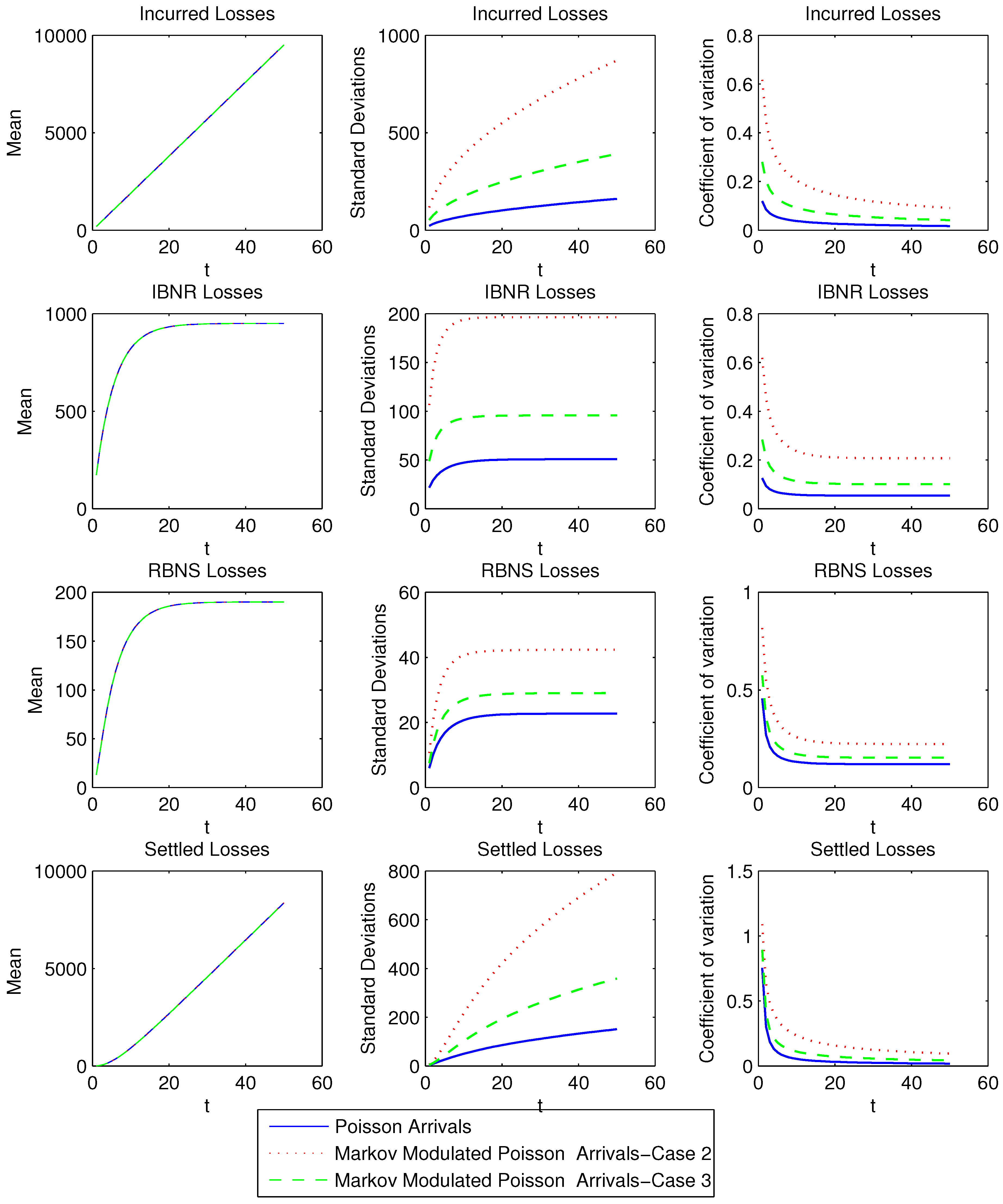
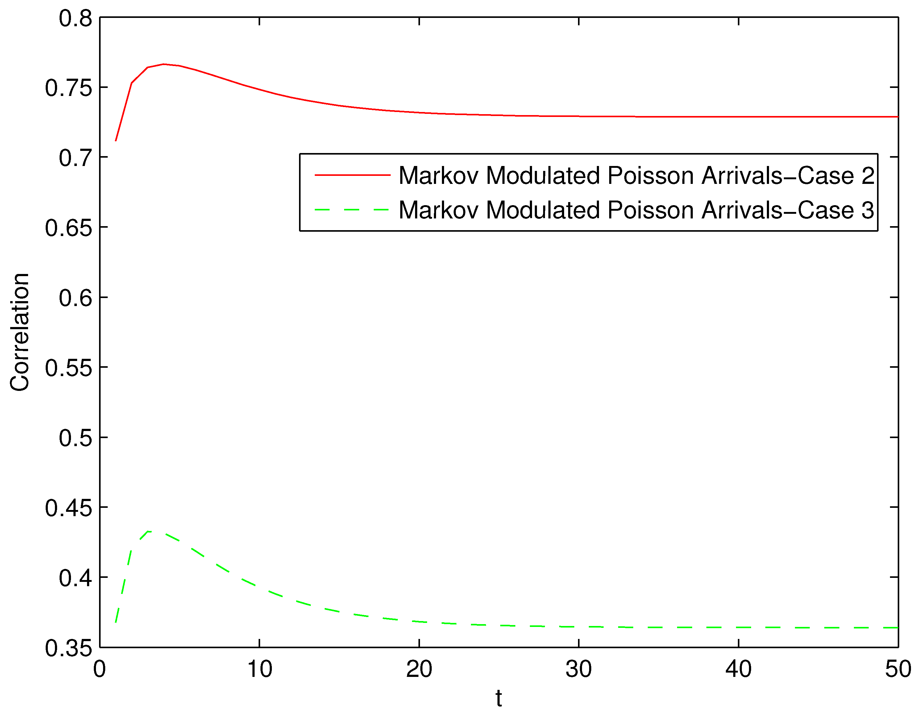
The mean, standard deviation and the coefficient of variation of the amount of the IBNR, RBNS and Settled claims for the three cases are computed using the formulas developed in Section 4. The values are plotted in Figure 1, from which it can be seen that the mean amount of IBNR, RBNS and Settled claims coincide in the three cases, however the standard deviations and the values of the coefficient of variation are very different. For case 1, IBNR and RBNS losses are independent because of the Poisson arrival assumption. However, as shown in Figure 2, the amount of IBNR and RBNS claims in case 2 and 3 are correlated, with the correlation affected by the burstiness of the claim arrival process.

Figure 1. Moments of the claims in different stages.

Figure 2. Correlation between Incurred But Not Reported (IBNR) and Reported But Not Settled (RBNS) claims.

6. Conclusion and Discussions

In this paper, we propose and analyze a model of insurance claim occurrence, reporting and handling process based on Markovian arrival processes. This model generalizes the commonly used models assuming Poisson claim arrivals. It enables us to evaluate how the claim occurrence process may affect the volatilities and interdependencies of the amount claims in different stages of the loss reporting/handling process.

The model can be generalized in many ways. For example, in the current model, the claim severity is fixed at the time when it occurs and are independent of the claim reporting and setting process, the full amount is paid when a claim is settled. However, in reality, claim severity could change during the claim settling process due to reassessment. In fact, in the model introduced by Huynh et al. (2015) [12], it is assumed that the claim size may change during the claim setting (investigation) process. The Markovian model proposed in this paper could be generalized to consider this. For example, one could assume that each claim of size y is modified by a random factor $V_y$ with distribution function $f_{V_y}$ during its stay in the RBNS phases. With such modifications, Equation (3) becomes

$$\begin{array}{c}\mathbb{E}\left[e^{\xi ·\mathbf{X}\left(t\right)}|N\left(t\right)=n,\mathrm{and}\mathrm{for}i=1,\cdots n,T_i=t_i,Y_i=y_i\right]\hfill \\ =\prod _{i=1}^n\left(\sum _{k\in S_{IBNR}}{p}_k(t-t_i)e^{{\xi }_k{y}_i}+\sum _{k\in S_{RBNS}\bigcup S_S}{p}_k(t-t_i)e^{{\xi }_k{y}_i{V}_{y_i}}\right).\hfill \end{array}$$

(20)

Thus Equation (8) becomes

$${\mathbf{D}}_1^{*}(\xi ,t)=\sum _{k\in S_{IBNR}}{p}_k\left(t\right){\mathbf{D}}_f^{*}\left({\xi }_k\right)+\sum _{k\in S_{RBNS}\bigcup S_S}{p}_k\left(t\right)\int \int {\mathbf{D}}_f\left(y_i\right)e^{{\xi }_k{y}_{i}v}{f}_{V_{y_i}\left(v\right)dvd{y}_i}.$$

(21)

With this, the calculation of the moments can be carried out is a similar way as in Section 4.

It should be pointed out that parameter estimation for MAP processes is much more complicated than for a Poisson process. How to estimate parameters for the MAP claim arrival process based on observation of reported/paid losses is an interesting future research topic.