Elementary Bounds on the Ruin Capital in a Diffusion Model of Risk

Abstract

In a diffusion model of risk, we focus on the initial capital needed to make the probability of ruin within finite time equal to a prescribed value. It is defined as a solution of a nonlinear equation. The endeavor to write down and to investigate analytically this solution as a function of the premium rate seems not technically feasible. Instead, we obtain informative bounds for this capital in terms of elementary functions.

1. Introduction and Rationale

In this paper, we focus on the solutions (w.r.t. u and c) of the nonlinear equation

$${\psi }_t(u,c\mid \vartheta )=\alpha$$

(1)

where $\alpha >0$ is a sufficiently small number and ${\psi }_t(u,c\mid \vartheta )$ is the probability of ruin within finite time $t>0$ in the standard diffusion risk model, i.e., when the annual risk reserve at time $s⩾0$ is defined as

$$R_s=u+cs-V_s,V_s=\vartheta s+\sigma \left(\vartheta \right){\mathsf{W}}_s$$

(2)

Here $u>0$ is the initial risk reserve and $c>0$ is the premium rate. By ${\mathsf{W}}_s$, $s⩾0$, we denote a standard Brownian motion. The aggregate claims payout process $V_s$, $s⩾0$, is a diffusion with continuous time, starting at zero. Its drift coefficient is $\vartheta >0$ and diffusion coefficient is $\sigma \left(\vartheta \right)>0$. The variance is $\text{D}{V}_s={\sigma }^2\left(\vartheta \right)s$.

Bearing in mind the well known result for diffusion with linear drift (see, e.g., Equation 1.1.4 in Part II, Chapter 2 of [1]), we have in this model

$$\begin{array}{cc}\hfill {\psi }_t(u,c\mid \vartheta )& =\mathsf{P}\left\{\underset{0<s⩽t}{inf}[u+(c-\vartheta )s-\sigma \left(\vartheta \right){\mathsf{W}}_s]<0\right\}\hfill \\ & =1-{\Phi }_{(0,1)}\left({\displaystyle \frac{u}{\sigma \left(\vartheta \right)\sqrt{t}}}-\frac{(\vartheta -c)\sqrt{t}}{\sigma \left(\vartheta \right)}\right)+exp\left\{2\frac{u(\vartheta -c)}{{\sigma }^2\left(\vartheta \right)}\right\}\hfill \\ & \times {\Phi }_{(0,1)}\left(-{\displaystyle \frac{u}{\sigma \left(\vartheta \right)\sqrt{t}}}-\frac{(\vartheta -c)\sqrt{t}}{\sigma \left(\vartheta \right)}\right)\hfill \end{array}$$

(3)

Here ${\Phi }_{(0,1)}\left(x\right)$ and ${\phi }_{(0,1)}\left(x\right)$ are the standard normal c.d.f. and p.d.f. respectively.

The solution of Equation (1) with respect to u is called the α-level initial capital, or ruin capital. We denote it by $u_{\alpha ,t}(c\mid \vartheta )$. The solution with respect to c is called the α-level premium rate. We denote it by $c_{\alpha ,t}(u\mid \vartheta )$. Since (see Equation (3)) ${\psi }_t(0,c\mid \vartheta )\equiv 1$ for any $t>0$, and since ${\psi }_t(u,c\mid \vartheta )$ monotone decreases, as $u>0$ ($c>0$) increases, the solution $u_{\alpha ,t}(c\mid \vartheta )$ exists for all $0<\alpha <1$, but only small α are of interest. This solution is bounded from above by $u_{\alpha ,t}(0\mid \vartheta )>0$ and monotone decreases to zero, as c increases.

It is easy to see that for any $c>0$

$$c_{\alpha ,t}(u_{\alpha ,t}(c\mid \vartheta )\mid \vartheta )=c$$

(4)

and for any $u>0$

$$u_{\alpha ,t}(c_{\alpha ,t}(u\mid \vartheta )\mid \vartheta )=u$$

(5)

The inverse functions for both $u_{\alpha ,t}(c\mid \vartheta )$ and $c_{\alpha ,t}(u\mid \vartheta )$ obviously exist1. From Equation (4) and Equation (5), we have $u_{\alpha ,t}(c\mid \vartheta )=c_{\alpha ,t}^{-1}(c\mid \vartheta )$ for any $c>0$ and $c_{\alpha ,t}(u\mid \vartheta )=u_{\alpha ,t}^{-1}(u\mid \vartheta )$ for any $u>0$. So, enough is to focus on the ruin capital $u_{\alpha ,t}(c\mid \vartheta )$.

The idea to look at the dependence of the initial capital u on the premium rate c, or vice versa, holding the probability of ruin ${\psi }_t(u,c\mid \vartheta )$ at a prescribed level α, i.e., to use this probability merely as a binder, agrees with insurance regulation. In a nutshell, each insurance year the premium may be set within sensible limits, while the corresponding initial capital must be so large that the probability of ruin remains at a prescribed level.

Developing a sensible control over the years2, insurance managers are interested not in the probability of ruin as itself, but in a good balance between the control leverages, such as the initial capital and premium rate, which makes the solvency controllable. Typically, the expressions for the probability of ruin within finite time like Equation (3) are either absent or intractable, and the decision makers perform their calculations numerically3.

Even when an explicit formula like Equation (3) exists, to find $u_{\alpha ,t}(c\mid \vartheta )$ in an explicit form, using elementary functions, is a tremendous endeavor. This can not be done even in our diffusion model Equation (2). However, in order to develop a sensible control, we need to scrutinize the behavior of $u_{\alpha ,t}(c\mid \vartheta )$ for all possible values of $c>0$. To this end, we propose in this paper informative and elementary upper and lower bounds. These bounds are compound and give valuable information about $u_{\alpha ,t}(c\mid \vartheta )$ in the both cases of profitable ($c>\vartheta$) and unprofitable ($0<c<\vartheta$) risk reserve process. The fundamental observation underlying the proof in the former case is the convexity (concavity downward) of $u_{\alpha ,t}(c\mid \vartheta )$, as a function of c.

In [5], we have considered the similar problem in the classical Lundberg model. The classical Lundberg model yields the second exceptional case where the analytical expression for the probability of ruin within finite time is known. Unlike in [5], the bounds in this paper are given for each t rather than asymptotically, as $t\to \infty$.

The rest of the paper is arranged as follows.

In Section 2, we formulate some background results obtained previously.

In Section 3, we formulate the main results. The fundamental remark about convexity of $u_{\alpha ,t}(c\mid \vartheta )$ as a function of c, as $c>\vartheta$, is proved by showing that $\frac{{\partial }^2}{\partial c^2}{u}_{\alpha ,t}(c\mid \vartheta )$ is positive. To find this second derivative, we apply the implicit function theorem. The other technical tool are the inequalities for the Mill’s ratio proved in [6].

In Section 4, we formulate some auxiliary results.

2. Some Background Results

For completeness, we present a number of related results obtained in [2,3,4]. Because of lack of space we do not give details of their proof.

2.1. Some Equalities

We put ${\kappa }_{\gamma }={\Phi }_{(0,1)}^{-1}(1-\gamma )$ for $(1-\gamma )$-quantile ($0<\gamma <1$). If γ increases from 0 to $1/2$, i.e., $1-\gamma$ decreases from 1 to $1/2$, the quantile $k_{\gamma }$ monotone decreases from $+\infty$ to zero. By symmetry, we have $k_{1-\gamma }=-k_{\gamma }$ and $k_{1/2}=0$. For $u_{\alpha ,t}(\vartheta \mid \vartheta )$, we have the following representation4.

Theorem 1 (Theorem 2.1 in [2]) In the diffusion model Equation (2), the solution with respect to u of Equation (1), as $c=\vartheta$, is

$$u_{\alpha ,t}(\vartheta \mid \vartheta )=\sigma \left(\vartheta \right)\sqrt{t}{\kappa }_{\alpha /2}$$

For $u_{\alpha ,t}(c\mid \vartheta )$ and $c_{\alpha ,t}(u\mid \vartheta )$, we have the following representations.

Theorem 2 (Theorem 4.4 in [3]) In the diffusion model Equation (2), the solution with respect to u of Equation (1) is

$$u_{\alpha ,t}(c\mid \vartheta )=\left\{\begin{array}{cc}\sigma \left(\vartheta \right)\sqrt{t}\left[{\displaystyle \frac{(\vartheta -c)\sqrt{t}}{\sigma \left(\vartheta \right)}}+{\mathsf{U}}_{\alpha }\left({\displaystyle \frac{(\vartheta -c)\sqrt{t}}{\sigma \left(\vartheta \right)}}\right)\right],\hfill & c⩽\vartheta \hfill \\ \sigma \left(\vartheta \right)\sqrt{t}{\mathsf{U}}_{\alpha }\left({\displaystyle \frac{(\vartheta -c)\sqrt{t}}{\sigma \left(\vartheta \right)}}\right),\hfill & c>\vartheta \hfill \end{array}\right.$$

(6)

where the function ${\mathsf{U}}_{\alpha }\left(x\right)$ for $x<0$ satisfies the equation

$$1-{\Phi }_{(0,1)}({\mathsf{U}}_{\alpha }\left(x\right)-x)+exp\left\{2x{\mathsf{U}}_{\alpha }\left(x\right)\right\}{\Phi }_{(0,1)}(-{\mathsf{U}}_{\alpha }\left(x\right)-x)=\alpha$$

(7)

for $x⩾0$ satisfies the equation

$$1-{\Phi }_{(0,1)}\left({\mathsf{U}}_{\alpha }\left(x\right)\right)+exp\left\{2x[x+{\mathsf{U}}_{\alpha }\left(x\right)]\right\}{\Phi }_{(0,1)}(-2x-{\mathsf{U}}_{\alpha }\left(x\right))=\alpha$$

(8)

is continuous, positive for all x, monotone increasing, as x increases from $-\infty$ to 0, and monotone decreasing, as x increases from 0 to $+\infty$, and such that5

$$\underset{x\to -\infty }{lim}{\mathsf{U}}_{\alpha }\left(x\right)=0,{\mathsf{U}}_{\alpha }\left(0\right)={\kappa }_{\alpha /2},\underset{x\to +\infty }{lim}{\mathsf{U}}_{\alpha }\left(x\right)={\kappa }_{\alpha }$$

Corollary 1 (Theorem 2.1 in [4]) In the diffusion model Equation (2), the solution with respect to c of Equation (1) is

$$c_{\alpha ,t}(u\mid \vartheta )=\left\{\begin{array}{cc}\vartheta -{\displaystyle \frac{\sigma \left(\vartheta \right)}{\sqrt{t}}}\left({\displaystyle \frac{u-u_{\alpha ,t}(\vartheta \mid \vartheta )}{\sigma \left(\vartheta \right)\sqrt{t}}}+{\mathsf{G}}_{\alpha }\left({\displaystyle \frac{u}{\sigma \left(\vartheta \right)\sqrt{t}}}\right)\right),\hfill & u⩾u_{\alpha ,t}(\vartheta \mid \vartheta )\hfill \\ \vartheta -{\displaystyle \frac{\sigma \left(\vartheta \right)}{\sqrt{t}}}\left({\displaystyle \frac{\sigma \left(\vartheta \right)\sqrt{t}}{u}}{\mathsf{G}}_{\alpha }\left({\displaystyle \frac{u}{\sigma \left(\vartheta \right)\sqrt{t}}}\right)\right),\hfill & u<u_{\alpha ,t}(\vartheta \mid \vartheta )\hfill \end{array}\right.$$

where $u_{\alpha ,t}(\vartheta \mid \vartheta )=\sigma \left(\vartheta \right)\sqrt{t}{\kappa }_{\alpha /2}$ and the function ${\mathsf{G}}_{\alpha }\left(x\right)$, $x>0$, is continuous, monotone increasing, as x increases, and such that6

$$\underset{x\to 0}{lim}{\mathsf{G}}_{\alpha }\left(x\right)=\frac{ln\alpha }{2},{\mathsf{G}}_{\alpha }\left({\kappa }_{\alpha /2}\right)=0,\underset{x\to +\infty }{lim}{\mathsf{G}}_{\alpha }\left(x\right)={\kappa }_{\alpha /2}-{\kappa }_{\alpha }$$

(9)

For $x⩾{\kappa }_{\alpha /2}$, being positive, ${\mathsf{G}}_{\alpha }\left(x\right)$ is convex and satisfies the equation

$$\begin{array}{c}\hfill 1-{\Phi }_{(0,1)}({\kappa }_{\alpha /2}-{\mathsf{G}}_{\alpha }\left(x\right))+exp\left\{2x[x-{\kappa }_{\alpha /2}+{\mathsf{G}}_{\alpha }\left(x\right)]\right\}{\Phi }_{(0,1)}(-2x+{\kappa }_{\alpha /2}-{\mathsf{G}}_{\alpha }\left(x\right))=\alpha \end{array}$$

(10)

For $0<x<{\kappa }_{\alpha /2}$, being negative, ${\mathsf{G}}_{\alpha }\left(x\right)$ is concave and satisfies the equation

$$1-{\Phi }_{(0,1)}(x-{\mathsf{G}}_{\alpha }\left(x\right)/x)+exp\left\{2{\mathsf{G}}_{\alpha }\left(x\right)\right\}{\Phi }_{(0,1)}(-x-{\mathsf{G}}_{\alpha }\left(x\right)/x)=\alpha$$

(11)

Moreover, for $0<x<{\kappa }_{\alpha /2}$ we have

$${\mathsf{G}}_{\alpha }\left(x\right)⩽\left(1-{\displaystyle \frac{x}{{\kappa }_{\alpha /2}}}\right){\displaystyle \frac{ln\alpha }{2}}$$

(12)

Since the functions ${\mathsf{U}}_{\alpha }(·)$ and ${\mathsf{G}}_{\alpha }(·)$ can not be written explicitly, Theorem 2 and Corollary 1 do not give the explicit solutions of Equation (1).

2.2. Some Inequalities

The following upper and lower bounds on $u_{\alpha ,t}(c\mid \vartheta )$ follow from Theorem 2. They are illustrated in Figure 1.

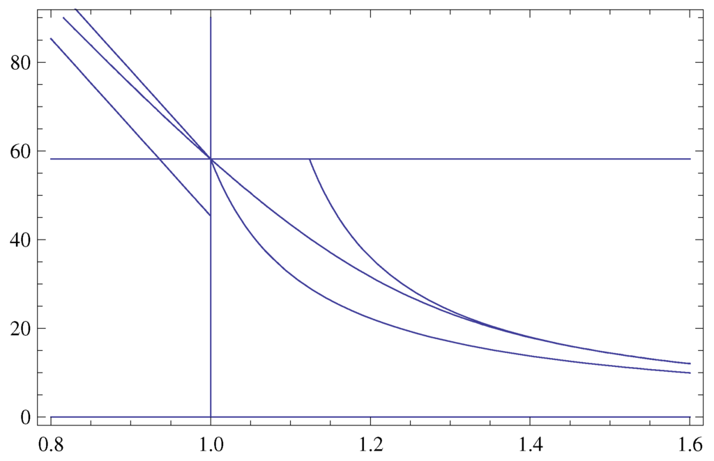
Figure 1. The function $u_{\alpha ,t}(c\mid \vartheta )$ of the variable $c>0$ (X-axis), as $\vartheta =1$, $\alpha =0.1$, $t=200$, and the bounds of Theorem 3. Horizontal line: $u_{\alpha ,t}(\vartheta \mid \vartheta )=\sigma \left(\vartheta \right)\sqrt{t}{\kappa }_{\alpha /2}$.

Figure 1. The function $u_{\alpha ,t}(c\mid \vartheta )$ of the variable $c>0$ (X-axis), as $\vartheta =1$, $\alpha =0.1$, $t=200$, and the bounds of Theorem 3. Horizontal line: $u_{\alpha ,t}(\vartheta \mid \vartheta )=\sigma \left(\vartheta \right)\sqrt{t}{\kappa }_{\alpha /2}$.

Theorem 3 In the diffusion model Equation (2), the solution with respect to u of Equation (1) is such that for $0<c<\vartheta$

$$\sigma \left(\vartheta \right)\sqrt{t}\left({\displaystyle \frac{(\vartheta -c)\sqrt{t}}{\sigma \left(\vartheta \right)}}+{\kappa }_{\alpha }\right)⩽u_{\alpha ,t}(c\mid \vartheta )⩽\sigma \left(\vartheta \right)\sqrt{t}\left({\displaystyle \frac{(\vartheta -c)\sqrt{t}}{\sigma \left(\vartheta \right)}}+{\kappa }_{\alpha /2}\right)$$

and for $c>\vartheta$

$$\begin{array}{c}\hfill -\frac{{\sigma }^2\left(\vartheta \right)ln\alpha }{2}{\left(c-\vartheta -\frac{\sigma \left(\vartheta \right)ln\alpha }{2\sqrt{t}{\kappa }_{\alpha /2}}\right)}^{-1}⩽u_{\alpha ,t}(c\mid \vartheta )⩽min\left\{u_{\alpha ,t}(\vartheta \mid \vartheta ),-\frac{{\sigma }^2\left(\vartheta \right)ln\alpha }{2}{\left(c-\vartheta \right)}^{-1}\right\}\end{array}$$

It is noteworthy (see Figure 1) that the upper bound for $c>\vartheta$ in Theorem 3 is compound: it is horizontal line until $u_{\alpha ,t}(\vartheta \mid \vartheta )<-\frac{1}{2}{\sigma }^2\left(\vartheta \right)ln\alpha {\left(c-\vartheta \right)}^{-1}$ and hyperbola otherwise. This hyperbola is the solution of the equation ${\psi }_{\infty }(u,c\mid \vartheta )=\alpha$.

The following upper and lower bounds on $c_{\alpha ,t}(u\mid \vartheta )$ follow from Corollary 1.

Corollary 2 (Corollary 2.1 in [4]) In the diffusion model Equation (2), the solution with respect to c of Equation (1) is such that for $0<u⩽u_{\alpha ,t}(\vartheta \mid \vartheta )$

$$\vartheta -{\displaystyle \frac{\sigma \left(\vartheta \right)}{\sqrt{t}}}\left({\displaystyle \frac{\sigma \left(\vartheta \right)\sqrt{t}}{u}}\left(1-{\displaystyle \frac{u}{u_{\alpha ,t}(\vartheta \mid \vartheta )}}\right){\displaystyle \frac{ln\alpha }{2}}\right)⩽c_{\alpha ,t}(u\mid \vartheta )⩽\vartheta -{\displaystyle \frac{\sigma \left(\vartheta \right)}{\sqrt{t}}}\left({\displaystyle \frac{\sigma \left(\vartheta \right)\sqrt{t}}{u}}\frac{ln\alpha }{2}\right)$$

and for $u>u_{\alpha ,t}(\vartheta \mid \vartheta )$

$$\vartheta -{\displaystyle \frac{\sigma \left(\vartheta \right)}{\sqrt{t}}}\left({\displaystyle \frac{u-u_{\alpha ,t}(\vartheta \mid \vartheta )}{\sigma \left(\vartheta \right)\sqrt{t}}}+{\kappa }_{\alpha /2}-{\kappa }_{\alpha }\right)⩽c_{\alpha ,t}(u\mid \vartheta )⩽\vartheta -{\displaystyle \frac{\sigma \left(\vartheta \right)}{\sqrt{t}}}\left({\displaystyle \frac{u-u_{\alpha ,t}(\vartheta \mid \vartheta )}{\sigma \left(\vartheta \right)\sqrt{t}}}\right)$$

3. The Main Results

In this section, our goal is to improve the upper bounds in Theorem 3, as $c>\vartheta$, and in Corollary 2, as $0<u⩽u_{\alpha ,t}(\vartheta \mid \vartheta )$. This improvement makes these rather rough upper bounds much more accurate and informative.

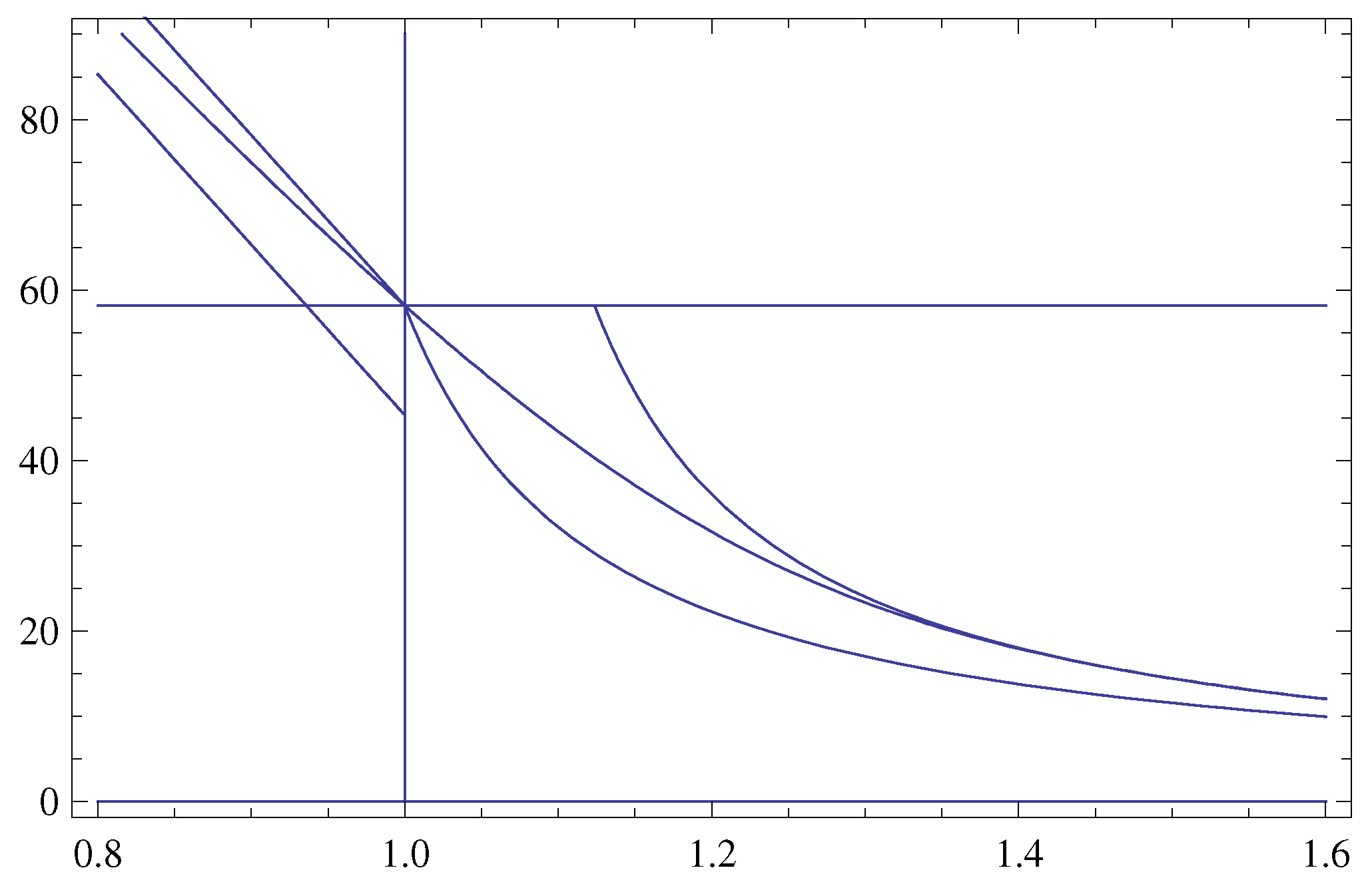
Our plan regarding Theorem 3 is as follows. First, for $c>\vartheta$, we prove the convexity (concavity downward) of $u_{\alpha ,t}(c\mid \vartheta )$, as a function of c. Then we enhance Theorem 3, as illustrated in Figure 2 and Figure 3. We draw the tangent line to hyperbola $-\frac{1}{2}{\sigma }^2\left(\vartheta \right)ln\alpha {\left(c-\vartheta \right)}^{-1}$ which is an upper bound for the ruin capital for $c>\vartheta$. Since $u_{\alpha ,t}(c\mid \vartheta )$ is a convex function of $c>\vartheta$, this tangent line is the required upper bound on $u_{\alpha ,t}(\vartheta \mid \vartheta )$ to the left of the point of tangency.

Figure 2. Graphs shown in Figure 1, with the graph of sloping straight line $t{\kappa }_{\alpha /2}^2(c-\vartheta )/(2ln\alpha )+\sigma \left(\vartheta \right)\sqrt{t}{\kappa }_{\alpha /2}$ starting from the point with abscissa ϑ and ordinate $u_{\alpha ,t}(\vartheta \mid \vartheta )=\sigma \left(\vartheta \right)\sqrt{t}{\kappa }_{\alpha /2}$, and tangent to the hyperbola $(-{\sigma }^2\left(\vartheta \right)ln\alpha )/\left(2(c-\vartheta )\right)$ at (right vertical line) $c=\vartheta -\sigma \left(\vartheta \right)ln\alpha /\left(\sqrt{t}{\kappa }_{\alpha /2}\right)$.

Figure 2. Graphs shown in Figure 1, with the graph of sloping straight line $t{\kappa }_{\alpha /2}^2(c-\vartheta )/(2ln\alpha )+\sigma \left(\vartheta \right)\sqrt{t}{\kappa }_{\alpha /2}$ starting from the point with abscissa ϑ and ordinate $u_{\alpha ,t}(\vartheta \mid \vartheta )=\sigma \left(\vartheta \right)\sqrt{t}{\kappa }_{\alpha /2}$, and tangent to the hyperbola $(-{\sigma }^2\left(\vartheta \right)ln\alpha )/\left(2(c-\vartheta )\right)$ at (right vertical line) $c=\vartheta -\sigma \left(\vartheta \right)ln\alpha /\left(\sqrt{t}{\kappa }_{\alpha /2}\right)$.

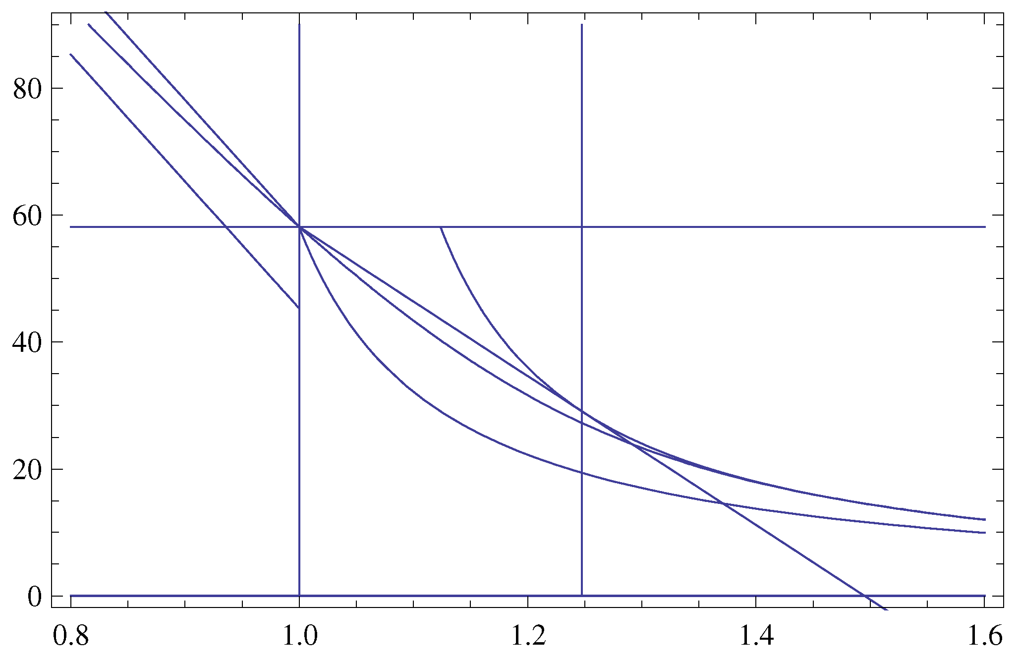
We formulate the following Theorem 4 which yields the improved upper bounds for $u_{\alpha ,t}(c\mid \vartheta )$, as $c>\vartheta$. It is illustrated in Figure 3. The proof of Theorem 4 is illustrated in Figure 2 and will be presented at the end of this section.

Figure 3. The function $u_{\alpha ,t}(c\mid \vartheta )$ of the variable $c>0$ (X-axis), as $\vartheta =1$, $\alpha =0.1$, $t=200$, and the bounds of Theorem 3 improved in Theorem 4.

Figure 3. The function $u_{\alpha ,t}(c\mid \vartheta )$ of the variable $c>0$ (X-axis), as $\vartheta =1$, $\alpha =0.1$, $t=200$, and the bounds of Theorem 3 improved in Theorem 4.

Theorem 4 In the diffusion model Equation (2), for $c>\vartheta$ we have

$$\begin{array}{c}\hfill u_{\alpha ,t}(c\mid \vartheta )⩽\left\{\begin{array}{cc}{\displaystyle \frac{t{\kappa }_{\alpha /2}^2}{2ln\alpha }}(c-\vartheta )+\sigma \left(\vartheta \right)\sqrt{t}{\kappa }_{\alpha /2},\hfill & \vartheta <c⩽\vartheta -{\displaystyle \frac{\sigma \left(\vartheta \right)ln\alpha }{\sqrt{t}{\kappa }_{\alpha /2}}}\hfill \\ -{\displaystyle \frac{{\sigma }^2\left(\vartheta \right)ln\alpha }{2}}{\left(c-\vartheta \right)}^{-1},\hfill & c>\vartheta -{\displaystyle \frac{\sigma \left(\vartheta \right)ln\alpha }{\sqrt{t}{\kappa }_{\alpha /2}}}\hfill \end{array}\right.\end{array}$$

The following result yields the improved upper bounds for $c_{\alpha ,t}(u\mid \vartheta )$, as $0<u<u_{\alpha ,t}(\vartheta \mid \vartheta )$.

Corollary 3 In the diffusion model Equation (2), for $0<u⩽u_{\alpha ,t}(\vartheta \mid \vartheta )$ we have

$$\begin{array}{c}\hfill c_{\alpha ,t}(u\mid \vartheta )⩽\left\{\begin{array}{cc}\vartheta -{\displaystyle \frac{{\sigma }^2\left(\vartheta \right)}{u}}{\displaystyle \frac{ln\alpha }{2}},\hfill & 0<u⩽{\displaystyle \frac{u_{\alpha ,t}(\vartheta \mid \vartheta )}{2}}\hfill \\ {\displaystyle \frac{2{\sigma }^2\left(\vartheta \right)ln\alpha }{u_{\alpha ,t}^2(\vartheta \mid \vartheta )}}(u-u_{\alpha ,t}(\vartheta \mid \vartheta ))+\vartheta ,\hfill & {\displaystyle \frac{u_{\alpha ,t}(\vartheta \mid \vartheta )}{2}}<u⩽u_{\alpha ,t}(\vartheta \mid \vartheta )\hfill \end{array}\right.\end{array}$$

The following result is fundamental.

Theorem 5 For $c>\vartheta$, the function $u_{\alpha ,t}(c\mid \vartheta )$ of the variable c is convex.

Proof of Theorem 5 It suffices to show that $\frac{{\partial }^2}{\partial c^2}{u}_{\alpha ,t}(c\mid \vartheta )>0$. Bearing in mind Equation (1), apply Theorem 6. We have

$$\frac{\partial }{\partial c}{u}_{\alpha ,t}(c\mid \vartheta )=-\frac{{\psi }_t^{(0,1)}(u,c\mid \vartheta ){|}_{u=u_{\alpha ,t}(c\mid \vartheta )}}{{\psi }_t^{(1,0)}(u,c\mid \vartheta ){|}_{u=u_{\alpha ,t}(c\mid \vartheta )}}$$

and7

$$\begin{array}{cc}\hfill \frac{{\partial }^2}{\partial c^2}& u_{\alpha ,t}(c\mid \vartheta )=-\frac{1}{{\left({\psi }_t^{(1,0)}(u,c\mid \vartheta ){|}_{u=u_{\alpha ,t}(c\mid \vartheta )}\right)}^3}\hfill \\ & \times \{{\psi }_t^{(0,2)}(u,c\mid \vartheta ){|}_{u=u_{\alpha ,t}(c\mid \vartheta )}{\left({\psi }_t^{(1,0)}(u,c\mid \vartheta ){|}_{u=u_{\alpha ,t}(c\mid \vartheta )}\right)}^2\hfill \\ & -2{\psi }_t^{(1,1)}(u,c\mid \vartheta ){|}_{u=u_{\alpha ,t}(c\mid \vartheta )}{\psi }_t^{(1,0)}(u,c\mid \vartheta ){|}_{u=u_{\alpha ,t}(c\mid \vartheta )}{\psi }_t^{(0,1)}(u,c\mid \vartheta ){|}_{u=u_{\alpha ,t}(c\mid \vartheta )}\hfill \\ & +{\psi }_t^{(2,0)}(u,c\mid \vartheta ){|}_{u=u_{\alpha ,t}(c\mid \vartheta )}{\left({\psi }_t^{(0,1)}(u,c\mid \vartheta ){|}_{u=u_{\alpha ,t}(c\mid \vartheta )}\right)}^2\}\hfill \end{array}$$

Bearing in mind Equation (3), introduce8

$$F(x,y)=1-{\Phi }_{(0,1)}(x+y)+exp\{-2xy\}{\Phi }_{(0,1)}(-x+y)$$

We have

$$\begin{array}{cc}\hfill {\psi }_t^{(1,0)}(u,c\mid \vartheta )& =\frac{1}{\sigma \left(\vartheta \right)\sqrt{t}}{F}^{(1,0)}(x,y){|}_{\begin{array}{c}x=\frac{u}{\sigma \left(\vartheta \right)\sqrt{t}}\\ y=-\frac{(\vartheta -c)\sqrt{t}}{\sigma \left(\vartheta \right)}\end{array}}\hfill \\ \hfill {\psi }_t^{(0,1)}(u,c\mid \vartheta )& =\frac{\sqrt{t}}{\sigma \left(\vartheta \right)}{F}^{(0,1)}(x,y){|}_{\begin{array}{c}x=\frac{u}{\sigma \left(\vartheta \right)\sqrt{t}}\\ y=-\frac{(\vartheta -c)\sqrt{t}}{\sigma \left(\vartheta \right)}\end{array}}\hfill \end{array}$$

and

$$\begin{array}{cc}\hfill {\psi }_t^{(2,0)}(u,c\mid \vartheta )& =\frac{1}{{\sigma }^2\left(\vartheta \right)t}{F}^{(2,0)}(x,y){|}_{\begin{array}{c}x=\frac{u}{\sigma \left(\vartheta \right)\sqrt{t}}\\ y=-\frac{(\vartheta -c)\sqrt{t}}{\sigma \left(\vartheta \right)}\end{array}}\hfill \\ \hfill {\psi }_t^{(1,1)}(u,c\mid \vartheta )& =\frac{1}{{\sigma }^2\left(\vartheta \right)}{F}^{(1,1)}(x,y){|}_{\begin{array}{c}x=\frac{u}{\sigma \left(\vartheta \right)\sqrt{t}}\\ y=-\frac{(\vartheta -c)\sqrt{t}}{\sigma \left(\vartheta \right)}\end{array}}\hfill \\ \hfill {\psi }_t^{(0,2)}(u,c\mid \vartheta )& =\frac{t}{{\sigma }^2\left(\vartheta \right)}{F}^{(0,2)}(x,y){|}_{\begin{array}{c}x=\frac{u}{\sigma \left(\vartheta \right)\sqrt{t}}\\ y=-\frac{(\vartheta -c)\sqrt{t}}{\sigma \left(\vartheta \right)}\end{array}}\hfill \end{array}$$

Furthermore9, for $x,y>0$

$$\begin{array}{cc}\hfill F^{(1,0)}(x,y)& =-2exp\{-2xy\}({\phi }_{(0,1)}(-x+y)+y{\Phi }_{(0,1)}(-x+y))<0\hfill \\ \hfill F^{(0,1)}(x,y)& =-2xexp\{-2xy\}{\Phi }_{(0,1)}(-x+y)<0\hfill \\ \hfill F^{(2,0)}(x,y)& =4yexp\{-2xy\}({\phi }_{(0,1)}(-x+y)+y{\Phi }_{(0,1)}(-x+y))\hfill \\ & +2xexp\{-2xy\}{\phi }_{(0,1)}(-x+y)\hfill \\ \hfill F^{(1,1)}(x,y)& =-2exp\{-2xy\}{\Phi }_{(0,1)}(-x+y)+4xyexp\{-2xy\}{\Phi }_{(0,1)}(-x+y)\hfill \\ & +2xexp\{-2xy\}{\phi }_{(0,1)}(-x+y)\hfill \\ \hfill F^{(0,2)}(x,y)& =2xexp\{-2xy\}(2x{\Phi }_{(0,1)}(-x+y)-{\phi }_{(0,1)}(-x+y))\hfill \end{array}$$

Direct algebraic manipulations yield

$$\begin{array}{c}{F}^{(0,2)}(x,y){\left(F^{(1,0)}(x,y)\right)}^2-2F^{(1,1)}(x,y)\left(F^{(1,0)}(x,y)F^{(0,1)}(x,y)\right)\hfill \\ \hfill +F^{(2,0)}(x,y){\left(F^{(0,1)}(x,y)\right)}^2=8x{\left(exp\{-2xy\}{\phi }_{(0,1)}(-x+y)\right)}^{3}D(x,y)\end{array}$$

(13)

where

$$D(x,y)=2y{M}^3(x-y)+(2+x^2-y^2)M^2(x-y)-2yM(x-y)-1$$

and (see Section 4.2)

$$M(x-y)=\frac{1-{\Phi }_{(0,1)}(x-y)}{{\phi }_{(0,1)}(x-y)}=\frac{{\Phi }_{(0,1)}(-x+y)}{{\phi }_{(0,1)}(-x+y)}$$

is Mill’s ratio. Note that

$$D(x,y)=D_1(x,y)+D_2(x,y)$$

where

$$D_1(x,y)=2x{M}^3(x-y)+2x(x-y)M^2(x-y)-2xM(x-y)$$

and

$$D_2(x,y)=-2(x-y)M^3(x-y)+(2-{(x-y)}^2)M^2(x-y)+2(x-y)M(x-y)-1$$

Prove that $D(x,y)>0$ for $x,y>0$. Bearing in mind that $1-wM\left(w\right)<M^2\left(w\right)$ and $M\left(w\right)>0$ for any finite w (see inequalities Equation (14)), it follows from

$$\begin{array}{cc}\hfill D_1(x,y)& =\left(2x{M}^3\left(w\right)+2xw{M}^2\left(w\right)-2xM\left(w\right)\right){|}_{w=x-y\in \mathsf{R}}\hfill \\ & =2x\left(M^2\left(w\right)+wM\left(w\right)-1\right)M\left(w\right){|}_{w=x-y\in \mathsf{R}}>0\hfill \end{array}$$

true for $x>0$, and from

$$\begin{array}{cc}\hfill D_2(x,y)& =\left(-2w{M}^3\left(w\right)+(2-w^2)M^2\left(w\right)+2wM\left(w\right)-1\right){|}_{w=x-y\in \mathsf{R}}\hfill \\ & =\left((1-wM\left(w\right))\left(2M^2\left(w\right)-(1-\left[wM\left(w\right)\right])\right)\right){|}_{w=x-y\in \mathsf{R}}\hfill \\ & >\left((1-wM(w\left)\right)\left(2\right(1-wM\left(w\right))-(1-wM\left(w\right)\left)\right)\right){|}_{w=x-y\in \mathsf{R}}\hfill \\ & =\left({(1-wM\left(w\right))}^2\right){|}_{w=x-y\in \mathsf{R}}>0\hfill \end{array}$$

We finally have for all $c>\vartheta$ and $u>0$

$$\frac{{\partial }^2}{\partial c^2}{u}_{\alpha ,t}(c\mid \vartheta )=-\frac{t^{3/2}}{\sigma \left(\vartheta \right)}\frac{D(x,y)}{{\left(F^{(1,0)}(x,y)\right)}^3}{|}_{\begin{array}{c}x=\frac{u}{\sigma \left(\vartheta \right)\sqrt{t}}\\ y=-\frac{(\vartheta -c)\sqrt{t}}{\sigma \left(\vartheta \right)}\end{array}}>0$$

and the proof is complete.

Proof of Theorem 4 Bearing in mind the convexity10 of $u_{\alpha ,t}(c\mid \vartheta )$ established in Theorem 5, apply Theorem 6 with $A=u_{\alpha ,t}(\vartheta \mid \vartheta )$, $B=(-{\sigma }^2\left(\vartheta \right)ln\alpha )/2$, $C=\vartheta$. We have the straight line

$$l\left(c\right)=-(A^2/4B)(c-C)+A={\displaystyle \frac{t{\kappa }_{\alpha /2}^2}{2ln\alpha }}(c-\vartheta )+\sigma \left(\vartheta \right)\sqrt{t}{\kappa }_{\alpha /2}$$

tangent to the hyperbola

$$h\left(c\right)=B/(c-C)=-{\displaystyle \frac{{\sigma }^2\left(\vartheta \right)ln\alpha }{2}}{\left(c-\vartheta \right)}^{-1}$$

This hyperbola is (see Theorem 3) the upper bound for $u_{\alpha ,t}(c\mid \vartheta )$, as $c>\vartheta$.

Abscissa and ordinate of the point of tangency are $\vartheta -\sigma \left(\vartheta \right)ln\alpha /\left(\sqrt{t}{\kappa }_{\alpha /2}\right)$ and $\sigma \left(\vartheta \right)\sqrt{t}{\kappa }_{\alpha /2}/2$. Taking the tangent line as the bound for $\vartheta <c⩽\vartheta -\sigma \left(\vartheta \right)ln\alpha /\left(\sqrt{t}{\kappa }_{\alpha /2}\right)$ and the hyperbola as the bound for $c>\vartheta -\sigma \left(\vartheta \right)ln\alpha /\left(\sqrt{t}{\kappa }_{\alpha /2}\right)$, we complete the proof.

Proof of Corollary 3 It follows straightforwardly from Theorem 4 and from the fact that $c_{\alpha ,t}(u\mid \vartheta )=u_{\alpha ,t}^{-1}(u\mid \vartheta )$ for any $u>0$.

4. Auxiliary Results

4.1. Mill’s Ratio

For finite x, Mill’s ratio is defined as

$$M\left(x\right)=\frac{1-{\Phi }_{\{0,1\}}\left(x\right)}{{\phi }_{\{0,1\}}\left(x\right)}=e^{x^2/2}{\int }_x^{\infty }{e}^{-t^2/2}dt$$

Evidently, $M\left(x\right)>0$ for all finite x. The most well-known results about Mill’s ratio are $M^{\prime }\left(x\right)=xM\left(x\right)-1<0$ and $M^{\prime \prime }\left(x\right)=M\left(x\right)(1+x^2)-x>0$, so $M\left(x\right)$ is convex and decreasing from ∞ to 0, as x increases from $-\infty$ to $+\infty$.

The inequalities11

$$0<1-xM\left(x\right)<M^2\left(x\right)$$

(14)

were proved in [6]. For this purpose, it has been observed that the function $e^{-t^2/2}/{\int }_x^{\infty }{e}^{-t^2/2}dt$ is a p.d.f. over the range $x⩽t<\infty$, and its variance is $1-\nu \left(x\right)\left(\nu \right(x)-x)$, where $\nu \left(x\right)=e^{-x^2/2}/{\int }_x^{\infty }{e}^{-t^2/2}dt$ is the reciprocal of Mill’s ratio. Since this must be positive for finite x, the inequality $\nu \left(x\right)\left(\nu \right(x)-x)<1$ follows. It is the upper limit in Equation (14).

4.2. Differentiation of Implicit Functions

The following implicit function theorem is well known in analysis (see e.g., Chapter I, § 5.2 and § 5.3 in [7]).

Theorem 6 Let F be a function that possesses partial derivatives up to second order continuous in some neighborhood of some solution, $(x_0,y_0)$, of the equation $F(x,y)=0$. If $F_2(x_0,y_0)\ne 0$, there are an $ϵ>0$ and a unique continuously differentiable function ϕ such that $\varphi \left(x_0\right)=y_0$ and $F(x,\varphi (x\left)\right)=0$ for $|x-x_0|<0$. Moreover, when $|x-x_0|<0$, we have

$${\varphi }^{\prime }\left(x\right)=-F^{(1,0)}(x,\varphi \left(x\right)){\left(F^{(0,1)}(x,\varphi \left(x\right))\right)}^{-1}$$

and

$$\begin{array}{c}{\varphi }^{\prime \prime }\left(x\right)=-(F^{(2,0)}(x,\varphi \left(x\right)){\left(F^{(0,1)}(x,\varphi \left(x\right))\right)}^2\hfill \\ -2F^{(1,1)}(x,\varphi \left(x\right))F^{(1,0)}(x,\varphi \left(x\right))F^{(0,1)}(x,\varphi \left(x\right))\\ \hfill +F^{(0,2)}(x,\varphi \left(x\right)){\left(F^{(1,0)}(x,\varphi \left(x\right))\right)}^2){\left({\left(F^{(0,1)}(x,\varphi \left(x\right))\right)}^3\right)}^{-1}\end{array}$$

4.3. Straight Line and Hyperbola

The following theorem is straightforward.

Theorem 7 For $A,B,C>0$, the straight line $l\left(x\right)=-(A^2/4B)(x-C)+A$ with a negative slope passing through the point with abscissa C and ordinate A, is tangent to the hyperbola $h\left(x\right)=B/(x-C)$ at the point with abscissa $2B/A+C$ and ordinate $A/2$.

References

- A.N. Borodin, and P. Salminen. Handbook of Brownian Motion. Facts and Formulæ. Basel, Switzerland: Birkhäuser, 1996. [Google Scholar]
- V.K. Malinovskii. “Zone-adaptive control strategy for a multiperiodic model of risk.” Ann. Actuar. Sci. 2 (2007): 391–409. [Google Scholar] [CrossRef]
- V.K. Malinovskii. “Scenario analysis for a multi-period diffusion model of risk.” ASTIN Bull. 39 (2009): 649–676. [Google Scholar] [CrossRef]
- V.K. Malinovskii. “Level premium rates as a function of initial capital.” Insur.: Math. Econ. 52 (2013): 370–380. [Google Scholar] [CrossRef]
- V.K. Malinovskii. “Improved asymptotic upper bounds on ruin capital in Lundberg model of risk.” Insur.: Math. Econ. 55 (2014): 301–309. [Google Scholar] [CrossRef]
- M.R. Sampford. “Some inequalities on Mill’s ratio and related functions.” Ann. Math. Stat. 24 (1953): 130–132. [Google Scholar] [CrossRef]
- D.V. Widder. Advanced Calculus. New York, NY, USA: Prentice-Hall, 1947. [Google Scholar]
- 1.Being the inverse function, is defined accordingly for . For completeness, it is set zero for .
- 2.In [2,3,4], the framework of this paper was embedded in the multi-year controlled diffusion models of risk and the controls were built annually, depending on the past years financial results.
- 3.This paper deals with analytical methods rather than numerical evaluation. There is no need to say about the difference between analytical and numerical analysis.
- 4.In what follows, we will make extensive use of both entries, and . It will not be difficult to convert into each other the expressions using either of these two forms.
- 5.Since , one has .
- 6.Recall that since , we have .
- 7.Here and in what follows, the symbols denote i-th and j-th partial derivatives of with respect to the first and the second variables, respectively.
- 8.Note that Equation (1) rewrites as where and .
- 9.To observe that for , note that . For , we have , which is positive since both summands are positive.
- 10.The graph of a convex function , , lies below the straight line connecting the points with abscissa and ordinate and with abscissa and ordinate , where and .
- 11.The lower limit in Equation (14) is easy. Since for finite x, the function is increasing from to 1, as x increases from to .
© 2014 by the authors; licensee MDPI, Basel, Switzerland. This article is an open access article distributed under the terms and conditions of the Creative Commons Attribution license (http://creativecommons.org/licenses/by/3.0/).