Article

Demand of Insurance under the Cost-of-Capital Premium Calculation Principle

1
Department of Business Administration, University of Hamburg, 20146 Hamburg, Germany
2
RiskLab, Department of Mathematics, ETH Zurich, 8092 Zurich, Switzerland
3
Swiss Finance Institute SFI Professor, 8006 Zurich, Switzerland
*
Author to whom correspondence should be addressed.
Risks 2014, 2(2), 226-248; https://doi.org/10.3390/risks2020226
Submission received: 11 March 2014 / Revised: 28 May 2014 / Accepted: 4 June 2014 / Published: 17 June 2014

Abstract

:
We study the optimal insurance design problem. This is a risk sharing problem between an insured and an insurer. The main novelty in this paper is that we study this optimization problem under a risk-adjusted premium calculation principle for the insurance cover. This risk-adjusted premium calculation principle uses the cost-of-capital approach as it is suggested (and used) by the regulator and the insurance industry.

1. Introduction

We study the problem of optimal insurance design. This is a risk sharing problem between an insured financial agent and an insurer who typically holds a whole portfolio of similar insured risks. There is a vast literature on this optimal insurance design problem, see for instance Arrow [1,2], Raviv [3], Gollier [4] and Gollier-Schlesinger [5]. Classical literature assumes that the preferences of both the insured and the insurer are modeled by the expected utility framework. Using this expected utility setting the Pareto optimal insurance design is determined. Usually, this results in choosing a deductible and co-insurance above this deductible. Raviv [3] investigates necessary and sufficient conditions leading to deductibles and co-insurance, and the cost of insurance is identified to be the driving force behind deductibles.
As described in Yaari [6] and Bernard et al. [7], this framework fails to explain various phenomena that are observed in practice, for instance, that financial agents prefer to purchase extended insurance cover for relatively small claims over buying protection against disastrous large claims. Bernard et al. [7] modify the original framework by introducing a probability distortion which tries to describe human behavior more appropriately. In particular, these probability distortions reflect that small and large claims are over-weighted by individuals which results in insurance covers different from deductibles.
In the present paper we choose a different approach for the modeling of the preferences of the insurer. In insurance practice, solvency of an insurance company is determined through a regulatory risk measure. This regulatory risk measure is the equity the insurance company needs to hold in order to run its business from a supervisory point of view. This risk measure is directly related to the insurance policies the company is selling and, henceforth, should directly reflect the quality of the insurance portfolio. The insurance company’s and the shareholders’ preferences, respectively, are then satisfied if the expected return on this regulatory risk measure, i.e., risk bearing equity, is sufficiently large.
In the present paper we model the regulatory risk measure with the expected shortfall risk measure (also called Tail-Value-at-Risk) as it is used in the Swiss Solvency Test [8]. Assuming that this risk measure reflects the necessary equity that needs to be provided by shareholders, the premium risk loading is model by a cost-of-capital approach which is equivalent to the expected return on this shareholders’ equity. In this spirit we obtain a risk-adjusted premium calculation principle which is the essential difference to the constant risk premium case considered in the literature, see formula (3’) in Raviv [3] or formula (2) in Bernard et al. [7]. As a result, the price of insurance will directly be related to the regulatory requirements and it will reflect the diversification within the insurance portfolio. The crucial result will be that insurance for small claims is comparatively cheap because it only marginally triggers the expected shortfall risk measure. This exactly explains that individuals purchase more insurance for small claims whereas insurance for large claims seems rather expensive in their judgment.
Organization of the paper. In the next section we introduce the insurance claim model which is based on a common risk factor that affects all claims simultaneously and idiosyncratic components that only influence individual claims. Based on this model we formulate the optimal insurance design problem from the viewpoint of the insured. In Section 3 we introduce the regulatory risk measure and we describe the related risk-adjusted premium calculation principle. The crucial point will be that idiosyncratic risk is diversifiable which substantially simplifies the regulatory risk measure and the related risk-adjusted premium calculation. Based on this risk-adjusted premium we determine the optimal insurance design in Section 4 and we conclude this section with various properties and examples of the optimal insurance design. All results and statements are proved in the appendix.

2. Insurance Model and Utility Optimization

We assume that the financial market has N financial agents, each of them facing a random claim X i , i = 1 , , N , where N is fixed but large. The random claims X i are driven by a common (latent) risk factor Θ and an idiosyncratic risk component Y i . For simplicity we assume product structure between these two risk drivers, i.e., X i = Θ Y i for i = 1 , , N . The common risk factor Θ can be interpreted as an external factor (like inflation, economic factor, legal changes or environmental factor) that affects all claims X i simultaneously, and the remaining risk drivers Y i are of idiosyncratic nature. We analyze the demand of insurance against these random claims. This brings us to the following model assumptions:
Assumptions 1 (insurance claim model). The insurance claims are given by X i = Θ Y i , for i = 1 , , N , with
  • Θ , Y 1 , , Y N are independent, strictly positive, P -a.s.,
  • Y i are i.i.d. with continuous and strictly positive density f Y on R + having finite mean;
  • Θ has bounded, continuous and strictly positive density f Θ supported on the interval T = ( θ 0 , θ 1 ) , with 0 < θ 0 < θ 1 < .
Note that many of the statements below can be formulated in much more generality, the elegance of Assumptions 1 is that they allow for nice interpretations and analytical results. Our aim is to study the demand of insurance cover against these random claims X i . Therefore, we need to study the following ingredients:
  • The insurance pricing functional π : X π ( X ) needs to be defined. We introduce π based on probability distortions in the spirit of Section 2.6.2 in Wüthrich et al. [9] and Section 8.2.6 in Wüthrich-Merz [10]. This is different from the classical treatment in the literature where the premium is often either chosen to be proportional to the expected claim E [ X ] or assessed using the expected utility framework, see Arrow [2], Raviv [3], Gollier-Schlesinger [5] and Bernard et al. [7]. Our approach will provide a risk-adjusted premium principle as it is required in the insurance industry for solvency considerations.
  • The possible insurance covers I : x I ( x ) need to be described.
  • The utility optimization problem of each agent i = 1 , , N needs to be characterized.
  • The influence of the common (non-diversifiable) risk driver Θ needs to be analyzed.
We start with the description of the individual utility optimization problem. We consider N homogeneous risk-averse financial agents all having twice differentiable, increasing and concave utility function u satisfying the Inada conditions (see also Assumptions 2 below). Moreover, each agent has the same initial wealth w 0 > 0 . The optimal insurance cover I of agent i is then obtained by the solution of the optimization problem
max I I E u w 0 X i + I ( X i ) π ( I ( X i ) )
where
  • I is the set of measurable non-decreasing functions I : R + R + with 0 I ( x ) x for all x R + and R ( x ) = x I ( x ) is non-decreasing. The latter is needed to prevent from moral hazard;
  • I ( X i ) describes the ceded claim, i.e., financial agent i faces retention R ( X i ) = X i I ( X i ) after insurance, note that we drop the index I i = I in the insurance cover because of homogeneity in i = 1 , , N ,
  • π ( I ( X i ) ) is the price for the insurance cover I ( X i ) .
We consider the homogeneous situation in Equation (1). This will allow to determine the equilibrium. A heterogeneous situation may be analyzed by applying perturbation theory to the homogeneous one.

3. The Regulatory Point of View

3.1. Aggregate Insurance Demand and Risk-Adjusted Premium

Assume for the time being that optimization problem (1) has a unique optimal solution I I . The aggregate insurance demand is then given by i = 1 N I ( X i ) . The model assumptions imply for any fixed insurance cover functional I I that the individual insurance demands I ( X i ) are i.i.d., conditionally given the latent risk factor Θ. Henceforth, the law of large numbers implies for the aggregate insurance demand (for any fixed I), conditional on Θ,
lim N 1 N i = 1 N I ( X i ) | { Θ } = E [ I ( X 1 ) | Θ ] = E I ( Θ Y 1 ) Θ = def . J I ( Θ ) , P - a . s .
For the function θ J I ( θ ) = E I ( Θ Y 1 ) Θ = θ we define the (left-continuous) generalized inverse J I as follows
J I ( x ) = inf θ T ; J I ( θ ) x
Lemma 1. Under Assumptions 1, the function θ J I ( θ ) is Lipschitz continuous and strictly increasing in θ T for any I I with I 0 . The generalized inverse x J I ( x ) is strictly increasing and continuous with J I ( J I ( x ) ) = x and J I ( J I ( θ ) ) = θ .
The lemma is proved in the appendix. Note that we need to exclude the case I 0 , however, this case is anyway not of interest to the insurance company, because no insurance cover is sold.
The law of large numbers (2) and Lemma 1 provide
lim N 1 N i = 1 N I ( X i ) < x = J I ( Θ ) < x = Θ < J I ( x ) , P - a . s .
We choose ε ( 0 , 1 ) . The Value-at-Risk (VaR) of Θ at security level 1 ε is given by the quantile
VaR 1 ε ( Θ ) = inf θ T ; F Θ ( θ ) 1 ε = F Θ ( 1 ε )
where F Θ denotes the distribution function of Θ. This and identity (3) now allow to analyze
P lim N 1 N i = 1 N I ( X i ) < J I VaR 1 ε ( Θ ) = P Θ < J I ( J I VaR 1 ε ( Θ ) ) = P Θ < VaR 1 ε ( Θ ) = 1 ε
where we also use absolute continuity of F Θ on T . In view of Equation (3), we may approximate the VaR for the aggregate insurance demand i = 1 N I ( X i ) by the VaR of Θ, i.e., for N large we approximate
P i = 1 N I ( X i ) < N J I VaR 1 ε ( Θ ) P lim N 1 N i = 1 N I ( X i ) < J I VaR 1 ε ( Θ ) = 1 ε
Therefore, the VaR of i = 1 N I ( X i ) on security level 1 ε is approximated by N J I ( VaR 1 ε ( Θ ) ) for large N. The interpretation of this is that idiosyncratic risks Y i are diversified in the insurance portfolio, but regulation needs to make sure that systemic risks Θ are controlled by a risk measure. This is a reasonable view for high frequency low severity insurance products. Note that the function J I depends on the explicit choice of the insurance cover functional I, however, the VaR of Θ does not depend on the choice of I which makes the approximation particularly attractive and allows to study insurance optimization.
For the premium calculation principle π we assume, according to insurance regulation practice, that the premium has two parts, the so-called pure risk premium and a risk-adjusted risk margin that should prevent from ruin. For the risk margin we use a cost-of-capital approach with the expected shortfall risk measure loading. This loading has the canonical risk margin allocation principle (see e.g., McNeil et al. [11]). Henceforth, we define the risk-adjusted premium π by
π ( I ( X i ) ) = E [ I ( X i ) ] + r CoC E I ( X i ) Θ > VaR 1 ε ( Θ ) E [ I ( X i ) ]
where r CoC ( 0 , 1 ) is the cost-of-capital rate and the excess claim E I ( X i ) Θ > VaR 1 ε ( Θ ) E [ I ( X i ) ] is the allocation of the total expected shortfall risk measure
ϱ = E i = 1 N I ( X i ) Θ > VaR 1 ε ( Θ ) N E [ I ( X 1 ) ]
to financial agent i. Due to approximation (4) this is a sensible risk-adjusted premium definition for large portfolio sizes N. As a consequence individual risk Y i is diversified within the portfolio and there only remains the (systemic) latent risk driver Θ which triggers the regulatory solvency capital ϱ.
Example 1. Assume that Y i are i.i.d. exponentially distributed with parameter c > 0 and that Θ 1 has an exponential distribution with parameter c = 1 . This implies that ( X 1 , , X N ) has a Clayton survival copula with heavy-tailed marginals, see Asimit et al. [12]. Note that in this example Θ does not have finite support as defined in Assumptions 1. This will simplify the calculations in this example, but does not harm the general considerations.
Assume that we buy full insurance cover I ( x ) = x . Then, we need to analyze i = 1 N X i = Θ i = 1 N Y i with i = 1 N Y i having a gamma distribution with parameters N and c. This implies for x > 0
P i = 1 N X i x = E P Θ 1 x 1 i = 1 N Y i i = 1 N Y i = E e x 1 i = 1 N Y i = c c + x 1 N
Therefore, we obtain VaR on security level 1 ε given by
VaR 1 ε i = 1 N X i = 1 c ( 1 ε ) 1 / N 1 ( 1 ε ) 1 / N = N E [ Y 1 ] 1 N ( 1 ε ) 1 / N 1
On the other hand we have for I ( x ) = x
N J I ( VaR 1 ε ( Θ ) ) = N E [ Y 1 ] VaR 1 ε ( Θ ) = N E [ Y 1 ] 1 log ( 1 ε ) 1
Thus, in this example the quality of approximation (4) is exactly determined by the speed of convergence of the Euler series log ( z ) = lim N N ( z 1 / N 1 ) for fixed z = ( 1 ε ) 1 .

3.2. Probability Distortion for the Cost-of-Capital Loading

The premium principle (5) can be rewritten with the help of probability distortions, see Example 8.16 in Wüthrich-Merz [10]. We define the probability distortion
φ = 1 r CoC + r CoC ε 1 { Θ > VaR 1 ε ( Θ ) }
Observe that choice r CoC [ 0 , 1 ) implies φ > 0 , P -a.s., and E [ φ ] = 1 . Therefore, φ is a probability distortion that allows for a change of probability measure. Moreover, this choice provides the insurance premium
π ( I ( X i ) ) = E φ I ( X i ) = E * [ I ( X i ) ]
where the pricing measure P * P is defined by the Radon-Nikodym derivative d P * / d P = φ .
Remark. For r CoC = 0 we have φ 1 and, henceforth, π ( I ( X i ) ) = E I ( X i ) . That is, the insurance company only asks for the pure risk premium. In the classical capital asset pricing model (CAPM) the latter occurs for uncorrelatedness of I ( X i ) with the market portfolio. The assumption r CoC > 0 is non-trivial and will be true for lines of business that have common economic risk factors with financial markets.
By a change of variable y = x / θ one sees that for θ T and x R + we have conditional density of X i , given Θ = θ ,
f ( x | θ ) = θ 1 f Y ( x / θ ) > 0
This provides marginal density of X i given by
f X ( x ) = T f ( x | θ ) f Θ ( θ ) d θ = T θ 1 f Y ( x / θ ) f Θ ( θ ) d θ > 0
note that due to Assumptions 1 the latter exists from Leibniz’ integral rule. This allows to define the function ψ : R + R + with
ψ ( x ) = ( 1 r CoC ) + r CoC ε { θ > VaR 1 ε ( Θ ) } f ( x | θ ) f Θ ( θ ) d θ f X ( x )
Theorem 1. Set Assumptions 1 and chose I I . We have premium identity
π ( I ( X i ) ) = E * [ I ( X i ) ] = E [ φ I ( X i ) ] = E ψ ( X i ) I ( X i )
The premium fulfills for any I I
π ( I ( X i ) ) E I ( X i )
This implies that the utility optimization problem (1) can be rewritten as
max I I E u w 0 X i + I ( X i ) E ψ ( X i ) I ( X i )
with ψ ( · ) given by Equation (7). In order to solve Equation (8) the properties of ψ will be crucial. Besides strict positivity and normalization E [ ψ ( X i ) ] = 1 we have for all non-decreasing functions T
E ψ ( X i ) T ( X i ) E [ ψ ( X i ) ] E T ( X i ) = E T ( X i )
this follows similar to the proof of Theorem 1, using the FKG inequality [13]. Unfortunately, the latter does not imply that ψ is monotone. However, monotonicity of ψ will be crucial in the further derivations. Therefore, we need more restrictive assumptions under which monotonicity holds.
Theorem 2. Set Assumptions 1 and assume that f Y is continuously differentiable. Assume that function g : R + R
y g ( y ) = y f Y ( y ) f Y ( y )
is non-increasing. Then ψ is a differentiable, non-decreasing function on R + .
Remark. The non-increasing property of g has to do with the concavity of the function z log f Y ( e z ) . Observe that
d d z log f Y ( e z ) = e z f Y ( e z ) f Y ( e z ) = g ( e z )
If g is non-increasing, then z log f Y ( e z ) is concave. Many common densities satisfy this property, for instance,
  • the gamma density on R + ,
  • the log-normal density on R + ,
  • the Pareto density on [ c , ) ,
  • the uniform density on [ 0 , 1 ] .
The normal density does not satisfy this property on R + if μ > 0 , it only satisfies the property on [ μ / 2 , ) . g is increasing if the density f Y has a too strong relative growth.
Example 2 (exponential distribution). Choose Y i expo ( c ) with c > 0 . The common factor Θ is chosen by f Θ ( θ ) = θ 1 1 { θ [ θ 0 , θ 1 ] } with θ 0 = 1 / ( e 1 ) and θ 1 = e / ( e 1 ) . Note that this is a density on [ θ 0 , θ 1 ] with E [ Θ ] = 1 . Finally, we set X i = Θ Y i . The function g is given by g ( y ) = c y and, hence, Theorem 2 applies. We calculate ψ. We have v = VaR 1 ε ( Θ ) = e 1 ε / ( e 1 ) (where the first equality defines v). This implies
v θ 1 θ 1 f Y ( x / θ ) f Θ ( θ ) d θ θ 0 θ 1 θ 1 f Y ( x / θ ) f Θ ( θ ) d θ = v θ 1 θ 2 exp c x θ 1 d θ θ 0 θ 1 θ 2 exp c x θ 1 d θ = exp c x ( e 1 ) / e exp c x ( e 1 ) / e 1 ε exp c x ( e 1 ) / e exp c x ( e 1 ) = 1 exp c x ( e 1 ) 2 e 1 ( e ε 1 ) / ( e 1 ) 1 exp c x ( e 1 ) 2 e 1
We define c 1 = c 1 ( c ) = c ( e 1 ) 2 e 1 and δ = ( e ε 1 ) / ( e 1 ) ( 0 , 1 ) and then we obtain
ψ ( x ) = ( 1 r CoC ) + r CoC ε 1 exp c 1 δ x 1 exp c 1 x
Observe that ψ is differentiable, strictly increasing with ψ ( 0 ) = ( 1 r CoC ) + r CoC ε δ and lim x = ( 1 r CoC ) + r CoC ε . In Figure 1 (lhs) we provide an example for the following numerical choices (i) r CoC = 6 % , this is the rate fixed in the Swiss Solvency Test, see Section 6.1 in [8]; (ii) c = 1 ; and (iii) ε = 5 % , this is higher than the Swiss Solvency Test shortfall probability of 1%. We choose this higher value because it helps to display the model features more clearly. Note that the cost-of-capital rate is understood as a risk premium because alternatively investors could also invest the amount of the risk measure in riskless funds.
Figure 1. Function x ψ ( x ) for parameters r CoC = 6 % and ε = 5 % : lhs: exponential Example 2 with c = 1 ; rhs: Gaussian Example 3 with μ = 4 .
Risks 02 00226 g001
Example 3 (Gaussian distribution). Choose Y i N ( μ , 1 ) with μ > 0 and Θ is chosen as in Example 2. In this case we obtain
ψ ( x ) = ( 1 r CoC ) + r CoC ε Φ ( x ( e 1 ) / e 1 ε μ ) Φ ( x ( e 1 ) / e μ ) Φ ( x ( e 1 ) μ ) Φ ( x ( e 1 ) / e μ )
In Figure 1 (rhs) we provide an example for the numerical choices r CoC = 6 % , ε = 5 % and μ = 4 . Observe that ψ is non-increasing in interval ( 0 , 2 ) .

4. Optimal Insurance Design

4.1. Optimal Control Problem and Fixed Insurance Premium

We analyze insurance optimization problem (8) step by step. We need to solve the problem
max I I 0 u w 0 x + I ( x ) P f X ( x ) d x
for premium P given by
P = π ( I ( X i ) ) = E ψ ( X i ) I ( X i ) = 0 ψ ( x ) I ( x ) f X ( x ) d x
In the first step we fix a premium P ( 0 , π ( X 1 ) ) and we relax the conditions on I in only requiring that the insurance cover fulfills 0 I ( x ) x , which is equivalent to requiring ( I ( x ) , x I ( x ) ) 0 . This optimization problem can be formulated as an optimal control problem which is solved using the technique from Kamien-Schwartz [14].
Assumptions 2. Set Assumptions 1. Moreover, we assume that ψ is differentiable, strictly increasing, bounded from below by ψ 0 = ψ ( 0 ) and bounded from above by ψ 1 = lim x ψ ( x ) . Utility function u fulfills the Inada conditions, i.e., u is twice differentiable, u > 0 , u < 0 , lim y y 0 u ( y ) = and lim y u ( y ) = 0 , where y 0 { , 0 } denotes the left endpoint of the domain of u.
Note that natural (not necessarily optimal) lower and upper bounds on ψ are 1 r CoC and 1 r CoC + r CoC / ε , respectively, see also Figure 1 (lhs). Therefore, the boundedness assumption does not pose an additional constraint on ψ.
Under these assumptions we reformulate and solve the modified optimization problem. Choose P ( 0 , π ( X 1 ) ) fixed; note that P { 0 , π ( X 1 ) } is trivial because it means no insurance and full insurance cover, respectively, is bought. Consider the following optimal control problem: find function i ( · ) : R + R + such that it maximizes
E u w 0 X 1 + i ( X 1 ) P = 0 u w 0 x + i ( x ) P f X ( x ) d x
subject to differential equation, see also Equation (10),
p ˙ ( x ) = ψ ( x ) i ( x ) f X ( x )
constraint
( i ( x ) , x i ( x ) ) 0
and initial and terminal condition
p ( 0 ) = 0 and p ( ) = P
Choose λ 0 and consider the Hamiltonian
H ( x , i , λ ) f X ( x ) = u ( w 0 x + i P ) λ i ψ ( x ) f X ( x )
Define
I ( x , λ ) = arg max i H ( x , i , λ ) , subject to ( i , x i ) 0 , see Equation ( 13 )
Lemma 2. Set Assumptions 2. Assume there exists λ 0 such that π ( I ( X 1 , λ ) ) = P , then I ( · , λ ) solves the optimal control problem (11)–(14).
There remains to calculate I ( · , λ ) and prove the existence of λ 0 such that terminal condition (14) holds. We define s 0 = s 0 ( x ) = w 0 x P and s 1 = w 0 P . Under Equation (13) we have
s 0 ( x ) w 0 x + i P s 1 and u ( s 0 ( x ) ) u ( w 0 x + i P ) u ( s 1 )
If the domain of u is R + we set s 0 ( x ) = ( w 0 x P ) 0 . We need to distinguish three different cases in Equation (15).
Case 1. λ ψ ( x ) u ( s 1 ) . In that case we buy full insurance cover, i.e.,
I ( x , λ ) = x
Case 2. u ( s 1 ) < λ ψ ( x ) < u ( s 0 ) . In that case we buy partial insurance cover because Equation (15) has an inner solution u ( w 0 x + i P ) = λ ψ ( x ) . This implies
I ( x , λ ) = ( u ) 1 ( λ ψ ( x ) ) w 0 + x + P
Case 3. u ( s 0 ) λ ψ ( x ) . In that case we buy no insurance cover, i.e.,
I ( x , λ ) = 0
If we summarize the three cases we get insurance cover
I ( x , λ ) = ( u ) 1 λ ψ ( x ) u ( s 0 ( x ) ) u ( s 1 ) w 0 + x + P = ( u ) 1 ( λ ψ ( x ) ) s 0 ( x ) s 1 w 0 + x + P = ( u ) 1 ( λ ψ ( x ) ) w 0 + x + P 0 x
For the existence of λ 0 which provides terminal condition (14) we have the following lemma.
Lemma 3. Set Assumptions 2. If the domain of u is R + we additionally assume for initial wealth w 0 > π ( X 1 ) .
(i) 
There exists a unique λ * = λ * ( P ) 0 such that π ( I ( X 1 , λ * ) ) = P ( 0 , π ( X 1 ) ) .
(ii) 
The function R ( x , λ ) = x I ( x , λ ) is non-decreasing in x, i.e., we do not have moral hazard.
(iii) 
For any P ( 0 , π ( X 1 ) ) there exists x 0 0 with
I ( x , λ * ) = x for all x x 0 and I ( x , λ * ) < x for all x > x 0
(iv) 
For any λ > 0 there exists a minimal x 1 0 such that
I ( x , λ ) > 0 f o r a l l x > x 1
(v) 
The function P λ * ( P ) is differentiable and strictly decreasing in P; and the function w 0 λ * ( P ) = λ * ( P , w 0 ) is differentiable and strictly decreasing in w 0 .
From Lemmas 2 and 3 we conclude that Equation (16) solves the optimal control problem (11)–(14) for fixed premium P and choice λ * = λ * ( P ) . There remains the optimization over all possible premiums P.
Example 4 (exponential utility function). We make an explicit choice for the utility function u. Fix α > 0 and consider exponential utility function
u ( y ) = 1 α exp α y
for y R . Observe that in this optimal control problem with exponential utility function the initial wealth w 0 has no influence on the optimization. Therefore w.l.o.g. we set w 0 = 0 . The Hamiltonian is then given by
H ( x , i , λ ) f X ( x ) = 1 α exp { α ( x + i P ) } λ i ψ ( x ) f X ( x ) = 1 α exp { α ( x + i ) } e α P λ i ψ ( x ) e α P f X ( x )
We set η = η ( λ , P ) = e α P λ . We need to maximize the following function over the set 0 i x , see Equation (13),
1 α exp { α ( x i ) } η i ψ ( x )
As above we have three different cases: Case 1. For η ψ ( x ) 1 we obtain I ( x , λ ) = x . Case 2. For 1 < η ψ ( x ) < e α x we obtain an inner solution
I ( x , η ) = x 1 α log η ψ ( x ) ( 0 , x )
Case 3. For e α x η ψ ( x ) we obtain I ( x , η ) = 0 .
Thus, if we summarize these three cases we have insurance cover
I ( x , η ) = x 1 α log η ψ ( x ) 0 x = x 1 { η ψ ( x ) e α x } 1 α log η ψ ( x ) 1 { 1 η ψ ( x ) e α x }
There remains to calculate η = η ( λ , P ) 0 such that premium requirement (14) is fulfilled. This is easier than in Lemma 3 because I ( x , η ) does not directly depend on P (only via η). Consider the function
η P * ( η ) = 0 ψ ( x ) I ( x , η ) f X ( x ) d x
For η ( 0 , ψ 1 1 ] we obtain P * ( η ) = π ( X 1 ) . On the interval ( ψ 1 1 , ) the premium P * ( η ) is continuous and strictly decreasing in η with limit lim η P * ( η ) = 0 . Therefore, we have continuous and strictly decreasing map
P * : ( ψ 1 1 , ) ( 0 , π ( X 1 ) ) , η P * ( η )
which provides for every η the corresponding premium P * ( η ) = π ( I ( X 1 , η ) ) ( 0 , π ( X 1 ) ) .
We calculate the derivative of the insurance cover in Case 2, i.e., on interval 1 < η ψ ( x ) < e α x ,
d d x I ( x , η ) = 1 1 α ψ ( x ) ψ ( x )
This is negative for all x with ψ ( x ) / ψ ( x ) > α . Therefore, for fixed premium P we may get insurance covers I ( · , λ * ( P ) ) which are decreasing on some intervals. Such an insurance cover does not lie in I .

4.2. Variable Insurance Premium

In Equations (11)–(14) we have studied the optimal control problem for a given fixed insurance premium P. There remains optimization over P [ 0 , π ( X 1 ) ] , i.e., consider the optimization problem
max P [ 0 , π ( X 1 ) ] U ( P ) = max P [ 0 , π ( X 1 ) ] E u w 0 X 1 + I ( X 1 , λ * ( P ) ) P
where we also use Equation (19) for the definition of U ( P ) . Note that U ( P ) is the optimal expected utility for fixed premium P. From Lemma 3 we know that for every P there exist x 0 = x 0 ( P ) 0 and x 1 = x 1 ( P ) 0 (maximal) such that
I ( x , λ * ( P ) ) = x for all x x 0 and I ( x , λ * ( P ) ) < x for all x > x 0
thus, full insurance cover is only bought on an interval [ 0 , x 0 ] ; and
I ( x , λ * ( P ) ) > 0 for all x > x 1
i.e., asymptotically no insurance cover is not optimal for fixed premium P.
If x 1 ( P ) = 0 we buy insurance cover for all positive claims and obtain expected utility
U ( P ) = 0 x 0 u w 0 P f X ( x ) d x + x 0 u ( u ) 1 ( λ * ( P ) ψ ( x ) ) f X ( x ) d x
with x 0 = x 0 ( P ) = ψ 1 ( u ( w 0 P ) / λ * ( P ) ) ψ 0 .
For x 1 ( P ) > 0 the situation is more sophisticated. We need to distinguish two cases.
Case (i): x 0 > 0 . In that case we have x 1 > x 0 (due to continuity) and we can choose a finite sequence x 0 = κ 0 ( P ) < κ 1 ( P ) < κ 2 ( P ) < κ 3 ( P ) < < κ 2 n ( P ) = x 1 such that for l 0
I ( x , λ * ( P ) ) = 0 on [ κ 2 l + 1 , κ 2 l + 2 ] and I ( x , λ * ( P ) ) ( 0 , x ) on ( κ 2 l , κ 2 l + 1 )
Case (ii): x 0 = 0 . In that case we have x 1 0 and we can choose a finite sequence 0 = κ 0 ( P ) = κ 1 ( P ) κ 2 ( P ) < κ 3 ( P ) < < κ 2 n ( P ) = x 1 such that for l 0
I ( x , λ * ( P ) ) = 0 on [ κ 2 l + 1 , κ 2 l + 2 ] and I ( x , λ * ( P ) ) ( 0 , x ) on ( κ 2 l , κ 2 l + 1 ) .
The optimal expected utility for given P then takes the form, set κ 2 n + 1 = ,
U ( P ) = 0 κ 0 u w 0 P f X ( x ) d x + l = 0 n κ 2 l κ 2 l + 1 u ( u ) 1 ( λ * ( P ) ψ ( x ) ) f X ( x ) d x
+ l = 0 n 1 κ 2 l + 1 κ 2 l + 2 u w 0 x P f X ( x ) d x
The first integral gives the contribution of full insurance cover, the second the one of partial insurance and the third one gives the contribution of no insurance to the total expected utility U ( P ) . This insurance cover I ( x , λ * ( P ) ) fulfills the premium identity, see Lemma 3,
P = 0 κ 0 ψ ( x ) x f X ( x ) d x + l = 0 n κ 2 l κ 2 l + 1 ψ ( x ) ( u ) 1 ( λ * ( P ) ψ ( x ) ) w 0 + x + P f X ( x ) d x
From the differentiability of the left-hand side of this identity we see that λ * ( P ) is a differentiable function in P, see also Lemma 3.
Theorem 3. Set Assumptions 2. If the domain of u is R + we additionally assume for initial wealth w 0 > π ( X 1 ) . The optimal expected utility P U ( P ) is a concave function on ( 0 , π ( X 1 ) ) with first derivative given by
U ( P ) = 0 κ 0 ( P ) λ * ( P ) ψ ( x ) u ( w 0 P ) f X ( x ) d x + l = 0 n 1 κ 2 l + 1 ( P ) κ 2 l + 2 ( P ) λ * ( P ) ψ ( x ) u ( w 0 x P ) f X ( x ) d x
This provides the following corollary:
Corollary 1. Set the assumptions of Theorem 3. Optimization problem (19) has a unique solution P * [ 0 , π ( X 1 ) ] and the optimal insurance cover is given by
I * ( x ) = I ( x , λ * ( P * ) )
where for P * = 0 we have I * ( x ) 0 , and for P * = π ( X 1 ) we have I * ( x ) = x for all x 0 .
There remains to analyze optimal insurance I * ( x ) , in particular, we analyze the question I * I . We already know from Lemma 3 that R * ( x ) = x I * ( x ) is non-decreasing and, hence, we do not have moral hazard in our model. There remains the analysis of the non-decreasing property of I * ( x ) .
Theorem 4. Set the assumptions of Theorem 3.
(i) 
Full insurance I ( x ) = x for all x is never optimal, that is, I * ( x ) x and P * < π ( X 1 ) .
(ii) 
No insurance I ( x ) 0 is never optimal, that is, I * ( x ) 0 and P * > 0 .
Theorems 3 and 4 immediately provide the nice consequences stated in the next corollary.
Corollary 2. Set the assumptions of Theorem 3.
(i) 
We always have an inner optimal premium P * ( 0 , π ( X 1 ) ) .
(ii) 
The optimal insurance I * can only have two types:
Type I: x 0 ( P * ) = x 1 ( P * ) = 0 , that is, I * ( x ) ( 0 , x ) for all x > 0 .
Type II: 0 < x 0 ( P * ) < x 1 ( P * ) , that is, co-existence of I * ( x ) = x and I * ( x ) = 0 .
(ii) 
If optimal insurance I * is of Type II, then it is non-monotone.
(iv) 
If optimal insurance I * is non-decreasing, then it is of Type I.
This corollary says that we always have an inner optimal premium P * ( 0 , π ( X 1 ) ) for optimization problem (19). The interplay between the insurance company’s pricing kernel ψ and the individual risk aversion in u will determine the monotonicity properties in the optimal insurance choice I * . This we are going to analyze next.
Consider the non-truncated insurance functional, see also Equation (16),
J ( x , λ ) = ( u ) 1 ( λ ψ ( x ) ) w 0 + x + P
Its derivative w.r.t. x is given by
d d x J ( x , λ ) = λ ψ ( x ) u ( u ) 1 ( λ ψ ( x ) ) + 1
Proposition 1. Set the assumptions of Theorem 3.
(i) 
Assume
inf λ u ( w 0 ) / ψ 1 inf x 0 d d x J ( x , λ ) 1 = inf λ u ( w 0 ) / ψ 1 inf x 0 λ ψ ( x ) u ( u ) 1 ( λ ψ ( x ) ) 1
Optimal insurance I * is of Type I and I * I .
(ii) 
Assume
sup λ u ( w 0 ) / ψ 1 d d x J ( x , λ ) 1 x = 0 = sup λ u ( w 0 ) / ψ 1 λ ψ ( 0 ) u ( u ) 1 ( λ ψ ( 0 ) ) < 1
Optimal insurance I * is of Type II and I * I .
We now provide an example that shows that optimal insurance I * can be either of Type I or of Type II depending on the risk aversion in u.
Example 5 (exponential utility). We revisit Example 4 and verify the two conditions of Proposition 1. Assume that β = sup x 0 ψ ( x ) / ψ ( x ) < . Fix α > 0 and consider exponential utility function given in Equation (17). In this case we have, see Equation (18),
d d x J ( x , λ ) 1 = 1 α ψ ( x ) ψ ( x ) 1
where the latter holds true for all α β = sup x 0 ψ ( x ) / ψ ( x ) . Thus, we have Type I optimal insurance I * for α sufficiently large.
On the other hand, for all α > 0 sufficiently small we have
d d x J ( x , λ ) 1 x = 0 = 1 α ψ ( 0 ) ψ ( 0 ) < 1
therefore, optimal insurance I * is of Type II.

4.3. Example and Interpretation

We revisit Examples 2 and 5. We choose Θ and Y i according to Example 2 this provides for the systemic component
E [ Θ ] = 1 , Var ( Θ ) = 0.0820 and Vco ( Θ ) = Var ( Θ ) 1 / 2 / E [ Θ ] = 29 %
this seems to be a comparably high value, but similar values may be reasonable, for instance, in business that is heavily driven by weather conditions. For the idiosyncratic component with c = 1 we have
E [ Y i ] = 1 , Var ( Y i ) = 1.0000 and Vco ( Y i ) = Var ( Y i ) 1 / 2 / E [ Y i ] = 100 %
This implies for insurance claim X i = Θ Y i
E [ X i ] = 1 , Var ( X i ) = 1.1640 and Vco ( X i ) = Var ( X i ) 1 / 2 / E [ X i ] = 108 %
We choose parameters r CoC = 6 % and ε = 5 % . For these choices we obtain ψ presented in Figure 1 (lhs). Moreover, we have β = sup x 0 ψ ( x ) / ψ ( x ) = 0.0301 . This implies that for exponential utility functions with α > β = 0.0301 we obtain Type I optimal insurance cover I * I . For the more extreme parameter choices r CoC = 8 % and ε = 1 % we obtain the constraint α > β = 0.0422 for Type I insurance, thus, the resulting β’s provide comparably weak constraints for Type I insurance. Note that there is an ongoing debate about appropriate values for r CoC . In a CAPM context r CoC = 6 % induces high correlations between our choice of Θ and the market portfolio, this seems debatable. On the other hand, some authors in the insurance literature argue that r CoC = 6 % is rather low, see for instance Section 4 in Pelsser [15] where the cost-of-capital rate is analyzed using various different pricing methods in incomplete markets.
If we consider the utility indifference price of X i for exponential utility function with risk aversion parameter α = 0.0422 (which corresponds to the Type I constraint for the choices r CoC = 8 % and ε = 1 % ) we obtain price
π α u ( X i ) = 1 α log E exp { α X i } = 1.0442
i.e., we obtain a loading of 4.42% which is very low. In typical non-life insurance contracts (private insurance) loadings are typically in the range of 20% to 30% which corresponds to a risk aversion parameter of roughly α = 0.2 . Therefore, typical risk aversion parameters of individual insureds fulfill α > β and will lead to Type I optimal insurance cover I * I .
Remarks.
  • Individual insured financial agents are typically willing to pay a loading in the range of 20% to 30%, i.e., this is a loading on a single insurance contract basis. The necessary risk margin from the insurer’s point of view is lower (due to the law of large numbers) and part of the margin paid by the insureds will be used to cover administrative costs at the insurance company.
  • The risk aversion parameters α from above seem to be low, but this is not necessarily the case and needs to be considered in more detail. Under our model assumptions we have, see also Equation (24),
    E exp { α X i } = E E exp { α Θ Y i } Θ = E c c α Θ
    for α θ 1 = α e / ( e 1 ) < c = 1 , and otherwise the above expectation is infinite. Therefore, we need to have α < 1 e 1 = 0.63 and otherwise we get an infinite price in Equation (24).
We give an example for α = 0.4 > β . In Figure 2 (lhs) we plot the optimal insurance cover x I ( x , λ * ( P ) ) for different fixed premiums P ( 0 , π ( X 1 ) ) . We see that all these insurance covers are of Type I because of α > β . They may have a deductible but they are non-decreasing. Figure 2 (rhs) shows that the optimal expected utility P U ( P ) is a concave function and therefore there is a unique optimal premium P * 0.97 . Thus, in this example we purchase quite a lot of insurance cover due to our comparably large risk aversion parameter α. In Figure 3 we provide the optimal insurance cover x I * ( x ) = I ( x , λ * ( P * ) ) for α = 0.4 (red line). We observe that we have Type I insurance with x 0 ( P * ) = x 1 ( P * ) = 0 .
Figure 2. Case of large individual risk aversion parameter α = 0.4 > β = 0.0301 : lhs: optimal insurance cover x I ( x , λ * ( P ) ) for different fixed premiums P ( 0 , π ( X 1 ) ) ; rhs: optimal expected utility P U ( P ) for different premiums P.
Risks 02 00226 g002
Figure 3. Case of large individual risk aversion parameter α = 0.4 > β = 0.0301 : the red line illustrates the optimal insurance cover x I * ( x ) = I ( x , λ * ( P * ) ) .
Risks 02 00226 g003
Figure 4. Case of small individual risk aversion parameter α = 0.01 < β = 0.0301 : lhs: optimal insurance cover x I ( x , λ * ( P ) ) for different fixed premium P ( 0 , π ( X 1 ) ) ; rhs: optimal expected utility P U ( P ) for different premium P.
Risks 02 00226 g004
Figure 5. Case of small individual risk aversion parameter α = 0.01 < β = 0.0301 : the red line illustrates the optimal insurance cover x I * ( x ) = I ( x , λ * ( P * ) ) .
Risks 02 00226 g005
We contrast the previous picture by the choice of a very small risk aversion parameter α = 0.01 < β (which results in a loading of 1.01% in Equation (24)). In Figure 4 (lhs) we plot the optimal insurance cover x I ( x , λ * ( P ) ) for different fixed premiums P ( 0 , π ( X 1 ) ) . We see that some of these insurance covers are of Type II because of α < β (in particular for small premiums P). Such insurance designs may simultaneously have full cover for small x and no insurance cover for larger x and, henceforth, are non-monotone. Figure 4 (rhs) shows that the optimal expected utility P U ( P ) is a concave function and therefore there is a unique optimal premium P * 0.27 . In this example, we buy only little insurance due to our small risk aversion parameter α = 0.01 . In Figure 5 we provide the optimal insurance cover x I * ( x ) = I ( x , λ * ( P * ) ) for α small (red line). We observe that we have Type II insurance with 0 < x 0 ( P * ) < x 1 ( P * ) because in our opinion insurance for small claims is rather cheap. Low prices for small claims (less than 1.09) are obtained because ψ ( x ) is strictly increasing with E [ ψ ( X 1 ) ] = 1 , ψ ( 0 ) = 0.9758 and ψ ( x ) < 1 for x < 1.09 (for our numerical choices). The latter is the case because small claims are only rarely triggered by large values of Θ and, therefore, are only marginally in the range of the expected shortfall risk measure of Θ. On the other hand, for larger claims we think that insurance cover is over-priced, note that the slope of ψ is rather steep on the interval x ( 0 , 50 ) , see Figure 1 (lhs). For this reason we buy no insurance on the interval ( 1.09 , 72 ] , and we start buying insurance again for very large claims exceeding threshold 72, see Figure 5, induced by risk aversion towards large claims.

4.4. Summary

We have studied optimal insurance designs of individual risk averse financial agents under the assumption of having a risk-adjusted insurance premium calculation principle. This risk-adjusted insurance premium calculation principle is based on the cost-of-capital method for the expected shortfall solvency risk measure. These considerations were enabled through the assumption that idiosyncratic risks are diversified within the insurance portfolio and the expected shortfall risk measure is only triggered by non-diversifiable systemic risks. This is a reasonable assumption for high frequency and low severity claims as they occur in private direct insurance. The findings were that optimal insurance designs in this framework will prevent for moral hazard, however, these insurance covers are not necessarily monotone due to the fact that the insured (depending on his risk aversion) may judge certain covers to be over-priced. However, for typical parameter settings this latter situation will not occur and, henceforth, optimal insurance covers will be monotone in the underlying insurance claims.

A. Proofs

Proof of Lemma 1. The function θ θ y is strictly increasing for all y R + . Since I I is a non-decreasing function, also the function θ I ( θ y ) is non-decreasing for all y R + . But then independence between Y 1 and Θ implies that also J I is non-decreasing. Assume there exist θ < θ such that
J I ( θ ) = E I ( Θ Y 1 ) Θ = θ = E I ( Θ Y 1 ) Θ = θ = J I ( θ )
Inequality I ( θ Y 1 ) I ( θ Y 1 ) , P -a.s., and identity (25) then imply that we must have I ( θ Y 1 ) = I ( θ Y 1 ) , P -a.s. Because the support of Y 1 is R + we must have that I is constant on R + , and from 0 I ( x ) x we see that this constant is equal to zero. Therefore, Equation (25) cannot occur unless I 0 . This proves the strict increasing property.
Next we prove Lipschitz continuity of J I . From R ( x ) = x I ( x ) non-decreasing it follows that for all ε > 0 and for all x R + we obtain (I is also non-decreasing)
0 I ( x ( 1 + ε ) ) I ( x ) = R ( x ) R ( x ( 1 + ε ) ) + ε x ε x
This implies that for any θ , θ > 0
I ( θ y ) I ( θ y ) θ θ y , for all y R +
and, moreover, using independence between Θ and Y 1 and integrability of Y 1 ,
J I ( θ ) J I ( θ ) = E I ( Θ Y 1 ) Θ = θ E I ( Θ Y 1 ) Θ = θ E I ( θ Y 1 ) I ( θ Y 1 ) θ θ E Y 1
Thus, the function J I is Lipschitz continuous and strictly increasing. As a consequence the remaining properties follow from Proposition A.3 in McNeil et al. [11]. This proves Lemma 1. ☐
Proof of Theorem 1. The first two premium identities follow from Equation (6). Choose a measurable function T : R + R . We obtain
E [ φ T ( X i ) ] = ( 1 r CoC ) E [ T ( X i ) ] + r CoC ε E T ( X i ) 1 { Θ > VaR 1 ε ( Θ ) }
We calculate the last term, using the tower property for conditional expectations in the first step,
E T ( X i ) 1 { Θ > VaR 1 ε ( Θ ) } = 1 { θ > VaR 1 ε ( Θ ) } T ( x ) f ( x | θ ) d x f Θ ( θ ) d θ = T ( x ) { θ > VaR 1 ε ( Θ ) } f ( x | θ ) f Θ ( θ ) d θ d x = T ( x ) { θ > VaR 1 ε ( Θ ) } f ( x | θ ) f Θ ( θ ) d θ f X ( x ) f X ( x ) d x
basically, this is simply the application of Bayes’ theorem. This implies that E [ φ T ( X i ) ] = E [ ψ ( X i ) T ( X i ) ] and proves the last identity for the choice T = I .
Next we prove the premium inequality. Choose I I . Observe that the function I : ( y , θ ) I ( θ y ) is component-wise non-decreasing. Moreover, the function φ : θ φ ( θ ) = 1 r CoC + r CoC ε 1 { θ > VaR 1 ε ( Θ ) } is also non-decreasing. Since Y i and Θ are independent, the FKG inequality implies, see Fortuin et al. [13],
π ( I ( X i ) ) = E φ I ( X i ) = E φ ( Θ ) I ( Θ Y i ) E φ ( Θ ) E I ( Θ Y i ) = E I ( Θ Y i ) = E I ( X i )
where in the second last step we have used that φ is a density and, thus, normalized. This closes the proof of Theorem 1. ☐
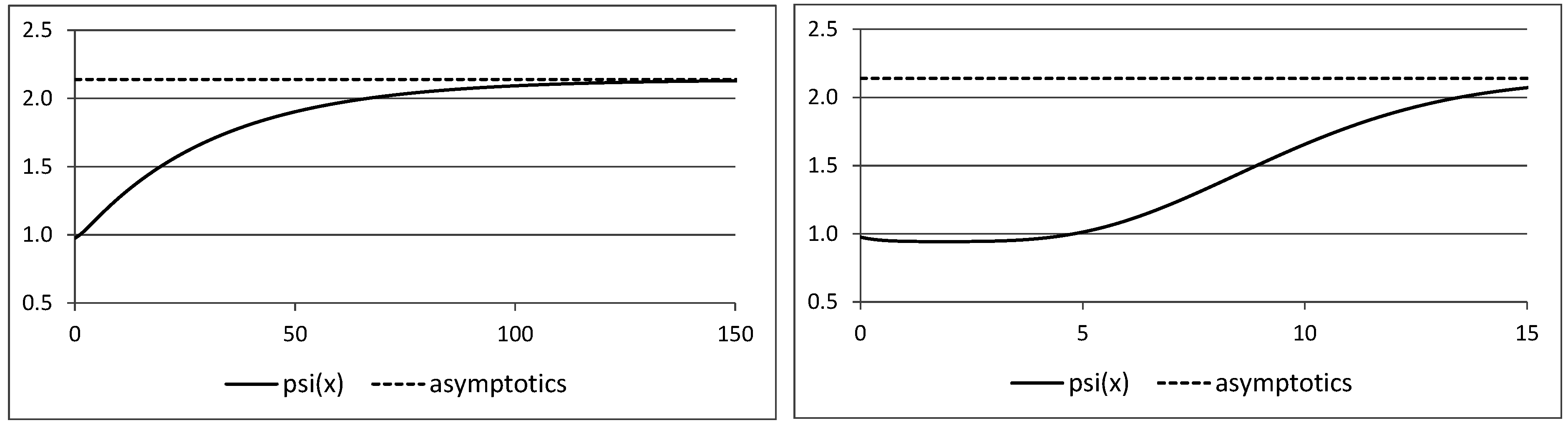
Proof of Theorem 2. For given x R + we recall Equation (7) which allows to rewrite ψ as follows, set v = VaR 1 ε ( Θ ) [ θ 0 , θ 1 ] ,
ψ ( x ) = ( 1 r CoC ) + r CoC ε v θ 1 θ 1 f Y ( x / θ ) f Θ ( θ ) d θ θ 0 θ 1 θ 1 f Y ( x / θ ) f Θ ( θ ) d θ
Differentiability of ψ follows from Leibniz’ integral rule. Moreover, we have
ψ ( x ) = r CoC ε v θ 1 θ 2 f Y ( x / θ ) f Θ ( θ ) d θ f X ( x ) v θ 1 θ 1 f Y ( x / θ ) f Θ ( θ ) d θ θ 0 θ 1 θ 2 f Y ( x / θ ) f Θ ( θ ) d θ f X ( x ) 2
We define the new probability measure P x by
d P x ( θ ) = θ 1 f Y ( x / θ ) f Θ ( θ ) d θ θ 0 θ 1 ϑ 1 f Y ( x / ϑ ) f Θ ( ϑ ) d ϑ = θ 1 f Y ( x / θ ) f Θ ( θ ) d θ f X ( x )
This allows to rewrite ψ ( x ) as follows: for Λ P x
ψ ( x ) = r CoC ε E x f Y ( x / Λ ) Λ f Y ( x / Λ ) 1 { Λ VaR 1 ε ( Θ ) } E x 1 { Λ VaR 1 ε ( Θ ) } E x f Y ( x / Λ ) Λ f Y ( x / Λ ) = r CoC ε E x g ( x / Λ ) x 1 { Λ VaR 1 ε ( Θ ) } E x 1 { Λ VaR 1 ε ( Θ ) } E x g ( x / Λ ) x
Observe that λ g ( x / λ ) and λ 1 { λ VaR 1 ε ( Θ ) } are non-decreasing. FKG inequality [13] then implies that ψ ( x ) 0 , which proves the claim. ☐
Proof of Lemma 2. The proof follows from Kamien-Schwartz [14]. Note that the optimal control problem in Kamien-Schwartz [14] is formulated on a finite interval [ 0 , 1 ] for x. This can be achieved by a change of variables x t / ( 1 t ) in Equations (11)–(14) and then one checks that all the conditions are fulfilled. ☐
Proof of Lemma 3. Note that we need to distinguish the two cases R and R + for the domain of u. In the latter case we need w 0 x + i P > 0 , due to lim y 0 u ( y ) = (Inada conditions). This implies that we need to have I ( x ) > x + P w 0 and, thus,
P = 0 ψ ( x ) I ( x ) f X ( x ) d x > 0 ψ ( x ) x + P w 0 f X ( x ) d x = π ( X 1 ) + P w 0
Therefore, the initial wealth w 0 should at least be able to finance the full insurance cover premium π ( X 1 ) if u has support R + . If the support of u is R the wealth w 0 x + i P is also allowed to become negative, and therefore no constraint is needed.
Proof of (i). Consider I ( x , λ ) given in Equation (16). Note that I ( x , λ ) is continuous and non-increasing in λ. Therefore, we would like to consider the limits λ 0 and λ of I ( x , λ ) . Note that sup x λ ψ ( x ) = λ ψ 1 . This implies for λ u ( s 1 ) / ψ 1 that
λ ψ ( x ) u ( s 0 ( x ) ) u ( s 1 ) u ( s 1 ) , for all x R +
and, hence, for λ u ( s 1 ) / ψ 1 we have
I ( x , λ ) = s 1 w 0 + x + P = x , for all x R +
This means that for λ u ( s 1 ) / ψ 1 we have π ( I ( X 1 , λ ) ) = π ( X 1 ) because we buy full insurance cover. On the other hand we have for any x R +
lim λ I ( x , λ ) = s 0 ( x ) w 0 + x + P = 0
i.e., we have point-wise (in x) convergence to 0. Using that 0 I ( x , λ ) x provides an integrable upper bound, we can apply Lebesgue’s dominated convergence theorem to obtain
lim λ π ( I ( X 1 , λ ) ) = lim λ 0 ψ ( x ) I ( x , λ ) f X ( x ) d x = 0
This immediately implies that there is λ ( u ( s 1 ) / ψ 1 , ) such that π ( I ( X 1 , λ ) ) = P ( 0 , π ( X 1 ) ) . Moreover, for λ ( u ( s 1 ) / ψ 1 , ) the function I ( x , λ ) is non-increasing in λ and on a set of positive Lebesgue measure it is strictly increasing, therefore π ( I ( X 1 , λ ) ) is strictly increasing in λ and hence, there is a unique λ * ( u ( s 1 ) / ψ 1 , ) with π ( I ( X 1 , λ * ) ) = P . This proves (i).
Proof of (ii). We consider
x I ( x , λ ) = ( u ) 1 λ ψ ( x ) u ( s 0 ( x ) ) u ( s 1 ) + w 0 P
The function λ ψ ( x ) u ( s 0 ( x ) ) = λ ψ ( x ) u ( w 0 x P ) is non-decreasing in x (note that we replace s 0 ( x ) by ( w 0 x P ) 0 if u has support R + ). This implies that ( u ) 1 λ ψ ( x ) u ( s 0 ( x ) ) u ( s 1 ) is non-increasing in x and, hence, the claim follows.
Proof of (iii). This is an immediate consequence of the increasing property of ψ ( · ) .
Proof of (iv). This is an immediate consequence of the boundedness of ψ ( · ) and the Inada condition at the left endpoint of u.
Proof of (v). From Equation (16) we get premium identity, see also Equation (21),
P = 0 ψ ( x ) I ( x , λ * ( P ) ) f X ( x ) d x = 0 ψ ( x ) ( u ) 1 ( λ * ( P ) ψ ( x ) ) w 0 + x + P 0 x f X ( x ) d x
Note that the bracket { · } is decreasing in w 0 . Therefore, ( u ) 1 ( λ * ( P ) ψ ( x ) ) needs to be increasing for the premium identity to be fulfilled. Since this increasing property needs to be strict on a set of positive Lebesgue measure for P ( 0 , π ( X 1 ) ) , λ * ( P ) = λ * ( P , w 0 ) is strictly decreasing in w 0 .
Observe from the premium identity
0 = 0 ψ ( x ) ( u ) 1 ( λ * ( P ) ψ ( x ) ) w 0 + x ( P ) ( x P ) f X ( x ) d x
Therefore, lower bound ( P ) and upper bound ( x P ) are strictly decreasing in P. This implies that the term ( u ) 1 ( λ * ( P ) ψ ( x ) ) needs to be increasing for the premium identity to be fulfilled. Since this increasing property needs to be strict on a set of positive Lebesgue measure we obtain that λ * ( P ) is strictly decreasing in P. ☐
Proof of Theorem 3. We start by calculating the derivative w.r.t. P in Equation (21). Observe that the derivatives at the boundaries vanish and we obtain
l = 0 n κ 2 l κ 2 l + 1 ψ ( x ) ( λ * ( P ) ) ψ ( x ) u ( u ) 1 ( λ * ( P ) ψ ( x ) ) + 1 f X ( x ) d x = 1 = 0 ψ ( x ) f X ( x ) d x
From this we immediately conclude that
l = 0 n κ 2 l κ 2 l + 1 ψ ( x ) ( λ * ( P ) ) ψ ( x ) u ( u ) 1 ( λ * ( P ) ψ ( x ) ) f X ( x ) d x = 0 κ 0 ψ ( x ) f X ( x ) d x + l = 0 n 1 κ 2 l + 1 κ 2 l + 2 ψ ( x ) f X ( x ) d x
We now calculate the derivative of U from Equation (20). This provides
U ( P ) = 0 κ 0 u w 0 P f X ( x ) d x + l = 0 n κ 2 l κ 2 l + 1 λ * ( P ) ψ ( x ) ( λ * ( P ) ) ψ ( x ) u ( u ) 1 ( λ * ( P ) ψ ( x ) ) f X ( x ) d x l = 0 n 1 κ 2 l + 1 κ 2 l + 2 u w 0 x P f X ( x ) d x
Using Equation (27) for the middle term on the right-hand side of the above identity provides the claimed derivative of U. The second derivative of U is then given by (observe that the derivatives at the boundaries vanish)
U ( P ) = 0 κ 0 ( P ) ( λ * ( P ) ) ψ ( x ) + u ( w 0 P ) f X ( x ) d x + l = 0 n 1 κ 2 l + 1 ( P ) κ 2 l + 2 ( P ) ( λ * ( P ) ) ψ ( x ) + u ( w 0 x P ) f X ( x ) d x
Both λ * ( P ) and u are decreasing which immediately implies that U ( P ) < 0 and we have concavity. ☐
Proof of Theorem 4. Consider the function
J ( x , λ * ( P ) ) = ( u ) 1 ( λ * ( P ) ψ ( x ) ) w 0 + x + P , with I ( x , λ * ( P ) ) = J ( x , λ * ( P ) ) 0 x .
The first derivative w.r.t. P is given by
d d P J ( x , λ * ( P ) ) = ( λ * ( P ) ) ψ ( x ) u ( u ) 1 ( λ * ( P ) ψ ( x ) ) + 1
From Lemma 3 we know that λ * ( P ) is decreasing in P, this implies that J ( x , λ * ( P ) ) and, henceforth, insurance cover I ( x , λ * ( P ) ) are non-decreasing in P for all x.
Proof of (i). Full insurance cover means that P = π ( X 1 ) . Therefore, we need to have point-wise convergence
lim P π ( X 1 ) I ( x , λ * ( P ) ) = x
because otherwise we would get the following contradiction
lim P π ( X 1 ) 0 ψ ( x ) I ( x , λ * ( P ) ) f X ( x ) d x < π ( X 1 )
This point-wise convergence requires for all x > 0
lim P π ( X 1 ) ( u ) 1 ( λ * ( P ) ψ ( x ) ) w 0 + P 0
which implies
lim P π ( X 1 ) λ * ( P ) ψ 1 u ( w 0 π ( X 1 ) )
The latter implies that x 0 ( P ) as P π ( X 1 ) . We prove this by contradiction: assume that x 0 ( P ) is bounded by y 0 . Choose y 1 > y 0 . Continuity and strict monotonicity of all involved functions implies that there exists P sufficiently close to π ( X 1 ) such that for all x y 1
λ * ( P ) ψ ( x ) < u ( w 0 P )
This implies that x 0 ( P ) y 1 , which is a contradiction. Moreover, this also implies that x 1 ( P ) = 0 for all P sufficiently large. Theorem 3 then reads as
U ( P ) = 0 κ 0 ( P ) λ * ( P ) ψ ( x ) u ( w 0 P ) f X ( x ) d x
Note that for any x < x 0 ( P ) = κ 0 ( P ) we have λ * ( P ) ψ ( x ) < λ * ( P ) ψ ( x 0 ) = u ( w 0 P ) which implies that U ( P ) < 0 for all P sufficiently close to π ( X 1 ) . Therefore, full insurance cover is never optimal.
Proof of (ii). If y 0 = 0 we need to have I ( x ) x w 0 which immediately provides the claim. Therefore, we can concentrate on y 0 = . No insurance means that P = 0 . In that case we need to have λ * ( P ) as P 0 . We prove this by contradiction. Assume that lim P 0 λ * ( P ) = λ 1 < . In that case we have
sup P > 0 sup y > 0 λ * ( P ) ψ ( y ) λ 1 ψ 1 < u ( s 0 ( x ) ) , for all x sufficiently large.
But this immediately implies that we buy insurance for all x sufficiently large, and hence P is bounded from below by a strictly positive constant. This contradicts P 0 . Therefore, we have
lim P 0 λ * ( P ) =
This implies that for any P sufficiently small we have
λ * ( P ) ψ ( x ) λ * ( P ) ψ 0 > u ( w 0 P )
This implies that for all P sufficiently small we have x 0 ( P ) = κ 0 ( P ) = 0 . In view of Theorem 3 this implies that U ( P ) > 0 for all P sufficiently small because the first integral in Theorem 3 is equal to zero. Therefore, no insurance is never optimal. ☐
Proof of Proposition 1. (i) From Theorem 4 we know that we cannot have full insurance cover if P * is optimal. This implies that λ * ( P * ) ψ 1 u ( w 0 P * ) u ( w 0 ) . Therefore, it is sufficient to consider λ u ( w 0 ) / ψ 1 . Condition (22) then implies that J ( x , λ ) is non-decreasing in any x and for all λ u ( w 0 ) / ψ 1 . Therefore, I ( · , λ ) I for all λ u ( w 0 ) / ψ 1 , which implies that I * is of Type I.
(ii) Condition (23) implies that J ( x , λ ) is strictly decreasing in 0, and henceforth, we have J ( x , λ ) < J ( 0 , λ ) for all x > 0 sufficiently close to 0. If J ( 0 , λ * ( P ) ) 0 then we have x 0 ( P ) = 0 and I ( x , λ * ( P ) ) = 0 for all x sufficiently close to 0, therefore P < P * . If J ( 0 , λ * ( P ) ) > 0 then I ( x , λ * ( P ) ) = x for all x sufficiently close to 0 and henceforth x 0 ( P ) > 0 which implies that I * is of Type II if P = P * . ☐

Author Contributions

Both authors contributed significantly to all aspects of this work.

Conflicts of Interest

The authors declare no conflict of interest.

References

  1. K.J. Arrow. “Uncertainty and the welfare economics of medical care.” Am. Econ. Rev. 53 (1963): 941–973. [Google Scholar]
  2. K.J. Arrow. Essays in the Theory of Risk Bearing. Chicago, IL, USA: Markham, 1971. [Google Scholar]
  3. A. Raviv. “The design of optimal insurance policy.” Am. Econ. Rev. 69 (1979): 84–96. [Google Scholar]
  4. C. Gollier. “Optimal insurance of approximate losses.” J. Risk Insur. 63 (1996): 369–380. [Google Scholar] [CrossRef]
  5. C. Gollier, and H. Schlesinger. “Arrow’s theorem on the optimality of deductibles: A stochastic dominance approach.” Econ. Theory 7 (1996): 359–363. [Google Scholar] [CrossRef]
  6. M. Yaari. “The dual theory of choice under risk.” Econometrica 55 (1987): 95–115. [Google Scholar] [CrossRef]
  7. C. Bernard, X.D. He, J.-A. Yan, and X.Y. Zhou. “Optimal insurance design under rank-dependent expected utility.” In Mathematical Finance. Waterloo, Canada: SSRN Preprint, 2014. [Google Scholar]
  8. Swiss Solvency Test. FINMA SST Technisches Dokument. Version 2; Bern, Switzerland: Swiss Solvency Test, October 2006. [Google Scholar]
  9. M.V. Wüthrich, H. Bühlmann, and H. Furrer. Market-Consistent Actuarial Valuation, 2nd ed. Berlin/Heidelberg, Germany: Springer, 2010. [Google Scholar]
  10. M.V. Wüthrich, and M. Merz. Financial Modeling, Actuarial Valuation and Solvency in Insurance. Berlin/Heidelberg, Germany: Springer, 2013. [Google Scholar]
  11. A.J. McNeil, R. Frey, and P. Embrechts. Quantitative Risk Management: Concepts, Techniques and Tools. Princeton, NJ, USA: Princeton University Press, 2005. [Google Scholar]
  12. A.V. Asimit, R. Vernic, and R. Zitikis. “Evaluating risk measures and capital allocations based on multi-losses driven by a heavy-tailed background risk: The multivariate Pareto-II model.” Risks 1 (2013): 14–33. [Google Scholar] [CrossRef] [Green Version]
  13. C.M. Fortuin, P.W. Kasteleyn, and J. Ginibre. “Correlation inequalities on some partially ordered sets.” Commun. Math. Phys. 22 (1971): 89–103. [Google Scholar] [CrossRef]
  14. M.I. Kamien, and N.L. Schwartz. “Sufficient conditions in optimal control theory.” J. Econ. Theory 3 (1971): 207–214. [Google Scholar] [CrossRef]
  15. A. Pelsser. Pricing in Incomplete Markets. Netspar Panel Papers, Volume 25; The Netherlands: Tilburg University, 2011. [Google Scholar]

