
Commodity Risk and Forecastability of International Stock Returns: The Role of Oil Returns Skewness


Abstract
1. Introduction
2. Variables and Methodology
2.1. Data
2.2. Econometric Model
3. Forecasting Results
4. Conclusions
Author Contributions
Funding
Institutional Review Board Statement
Informed Consent Statement
Data Availability Statement
Acknowledgments
Conflicts of Interest
Appendix A

| Full Sample | Ward War I [1914–1918]6 | Great Depression [1929–1941]7 | Ward War II [1939–1945]8 | OPEC Formation [September 1960–Present]9 | COVID-19 [December 2019–December 2023]10 | Invasion of Ukraine by Russia [February 2022–Present]11 | ||||||||
|---|---|---|---|---|---|---|---|---|---|---|---|---|---|---|
| G7 Countries + Switzerland | Oil Return | Stock Return | Oil Return | Stock Return | Oil Return | Stock Return | Oil Return | Stock Return | Oil Return | Stock Return | Oil Return | Stock Return | Oil Return | Stock Return |
| Canada (1915:01–2023:09) | 0.31 (7.00) | 0.40 (4.47) | 2.11 (4.26) | 0.18 (2.25) | −0.26 (5.75) | −0.67 (7.02) | 0.47 (3.42) | 0.33 (4.19) | 0.45 (8.00) | 0.49 (4.36) | 0.98 (16.91) | 0.37 (4.60) | 0.36 (8.44) | −0.28 (3.09) |
| France (1898:01–2023:09) | 0.33 (6.72) | 0.54 (5.1) | 0.78 (5.40) | 0.36 (3.59) | −0.26 (5.75) | 0.30 (6.64) | 0.47 (3.42) | 1.58 (7.15) | 0.45 (8.00) | 0.43 (5.21) | 0.98 (16.91) | 0.37 (5.51) | 0.36 (8.44) | −0.03 (3.89) |
| Japan (1914:08–2023:09) | 0.3 (7.0) | 0.55 (6.03) | 1.56 (4.68) | 1.15 (5.69) | −0.26 (5.75) | 0.32 (4.61) | 0.47 (3.42) | 0.09 (3.17) | 0.45 (8.00) | 0.43 (5.31) | 0.98 (16.91) | 0.74 (4.01) | 0.36 (8.44) | 0.98 (2.49) |
| Germany (1870:01–2023:09) | 0.15 (7.63) | 0.22 (7.03) | 0.78 (5.40) | −0.40 (6.40) | −0.26 (5.75) | −0.01 (4.04) | 0.47 (3.42) | 0.51 (1.61) | 0.45 (8.00) | 0.30 (5.07) | 0.98 (16.91) | 0.00 (5.61) | 0.36 (8.44) | −0.65 (4.40) |
| Italy (1905:02–2023:09) | 0.29 (6.80) | 0.42 (6.70) | 0.78 (5.40) | 0.18 (5.00) | −0.26 (5.75) | 0.23 (5.21) | 0.47 (3.42) | 1.97 (11.32) | 0.45 (8.00) | 0.25 (6.23) | 0.98 (16.91) | 0.42 (6.05) | 0.36 (8.44) | 0.01 (4.58) |
| UK (1859:10–2023:09) | 0.08 (9.28) | 0.28 (3.80) | 0.78 (5.40) | −0.21 (1.90) | −0.26 (5.75) | −0.18 (4.67) | 0.47 (3.42) | 0.50 (4.57) | 0.45 (8.00) | 0.48 (5.07) | 0.98 (16.91) | 0.07 (4.44) | 0.36 (8.44) | 0.05 (2.71) |
| USA (1859:10–2023:09) | 0.08 (9.28) | 0.41 (4.09) | 0.78 (5.40) | −0.03 (3.18) | −0.26 (5.75) | −0.62 (8.19) | 0.47 (3.42) | 0.37 (4.05) | 0.45 (8.00) | 0.58 (3.61) | 0.98 (16.91) | 0.76 (4.66) | 0.36 (8.44) | −0.18 (3.94) |
| Switzerland (1916:07–2023:09) | 0.27 (7.02) | 0.29 (4.30) | 1.44 (3.65) | −0.32 (2.00) | −0.26 (5.75) | −0.10 (5.20) | 0.47 (3.42) | 0.07 (3.06) | 0.45 (8.00) | 0.32 (4.51) | 0.98 (16.91) | 0.07 (3.87) | 0.36 (8.44) | −0.75 (3.12) |
| BRICS | ||||||||||||||
| Brazil (1954:02–2023:09) | 0.41 (7.62) | 5.19 (19.86) | - - | - - | - - | - - | - - | - - | 0.45 (8.00) | 5.47 (20.78) | 0.98 (16.91) | 0.18 (6.97) | 0.36 (8.44) | 0.45 (4.58) |
| Russia (1997:10–2023:09) | 0.48 (10.28) | 1.71 (10.45) | - - | - - | - - | - - | - - | - - | 0.48 (10.28) | 1.71 (10.45) | 0.98 (16.91) | 0.47 (7.85) | 0.36 (8.44) | −0.04 (10.15) |
| India (1921:07–2023:09) | 0.28 (6.98) | 0.48 (5.17) | - - | - - | −0.26 (5.75) | 0.20 (3.74) | 0.47 (3.42) | 0.92 (3.96) | 0.45 (8.00) | 0.79 (6.01) | 0.98 (16.91) | 1.08 (5.10) | 0.36 (8.44) | 0.56 (3.32) |
| China (1991:01–2023:09) | 0.32 (9.56) | 1.58 (14.76) | - | - | - | - | - | - | 0.32 (9.56) | 1.58 (14.76) | 0.98 (16.91) | 0.26 (4.27) | 0.36 (8.44) | −0.29 (4.49) |
| South Africa (1910:02–2024:05) | 0.30 (6.92) | 0.60 (4.46) | 0.78 (5.40) | 0.20 (2.48) | −0.26 (5.75) | 0.41 (3.88) | 0.47 (3.42) | 0.88 (2.69) | 0.45 (8.00) | 0.87 (5.38) | 0.98 (16.91) | 0.58 (4.79) | 0.36 (8.44) | −0.05 (3.55) |

| Crises | Date |
|---|---|
| Panic of 1866 | 1866 |
| Great Depression of British Agriculture | 1873–1896 |
| Long Depression | 1873–1896 |
| Panic of 1901 | 1901 |
| Panic of 1907 | 1907 |
| World War I | 1914–1918 |
| Depression of 1920–21 | 1920–1921 |
| Wall Street Crash of 1929 and Great Depression | 1929–1939 |
| World War II | 1939–1945 |
| OPEC oil price shock | 1973 |
| Energy crisis | 1979 |
| Secondary banking crisis | 1973–1975 |
| Early 1980s Recession | 1981–1982 |
| Latin American debt crisis | 1982 |
| Bank stock crisis | 1983 |
| Japanese asset price bubble | 1986–1992 |
| Black Monday | 1987 |
| Savings and loan crisis | 1986–1995 |
| Special Period in Cuba | 1990–1994 |
| India economic crisis | 1991 |
| Finnish banking crisis | 1991–1993 |
| Swedish banking crisis | 1990 |
| Economic crisis in Mexico | 1994 |
| Asian financial crisis | 1997 |
| Russian financial crisis | 1998 |
| Ecuador financial crisis | 1998–1999 |
| Argentine economic crisis | 1999–2002 |
| Samba effect | 1999 |
| Dot-com bubble | 2000-2002 |
| Turkish economic crisis | 2001 |
| Uruguay banking crisis | 2002 |
| Venezuelan general strike | 2002–2003 |
| Financial Crisis | 2007–2009 |
| 2000s energy crisis | 2003–2009 |
| Subprime mortgage crisis | 2007–2010 |
| United States housing bubble and United States housing market correction | 2003–2011 |
| Automotive industry crisis | 2008–2010 |
| Icelandic financial crisis | 2008–2012 |
| Irish banking crisis | 2008–2010 |
| Russian financial crisis | 2008–2009 |
| Latvian financial crisis | 2008 |
| Venezuelan banking crisis | 2009–2010 |
| Spanish financial crisis | 2008–2016 |
| European sovereign debt crisis | 2009–2018, and ongoing |
| Portuguese financial crisis | 2010–2014 |
| Crisis in Venezuela | 2012–2018, and ongoing |
| Ukrainian crisis | 2013–2014 |
| Russian financial crisis | 2014 |
| Brazilian economic crisis | 2014–2017 |
| Chinese stock market crash | 2015 |
| Turkish currency and debt crisis | 2018 |
| Debt crisis in India | 1993–2018, and ongoing |
| COVID-19 Pandemic | 2020 |
| Russia–Ukraine War | 2022, and ongoing |
| Israel–Hamas War | 2023 |
| 1 | |
| 2 | Stock price data for the UK and the US in fact starts from 1693:01 and 1791:08, respectively. |
| 3 | https://globalfinancialdata.com/ (accessed on 1 June 2023). |
| 4 | The rationale for multiple forecast horizons is to ensure robustness while capturing short-, medium-, and longer-term effects, and providing a comprehensive understanding of how oil price skewness influences stock return over varying time scales. |
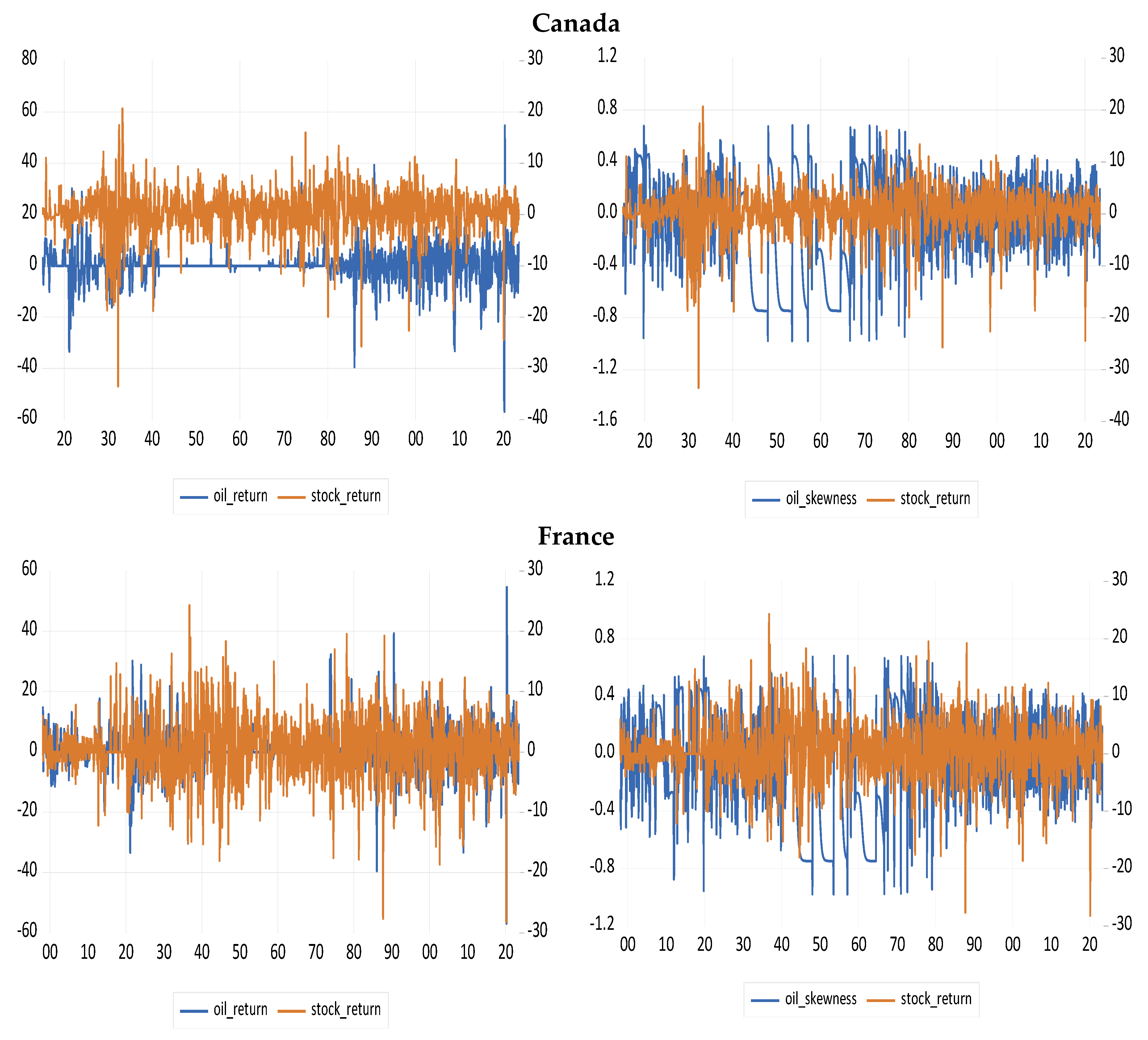
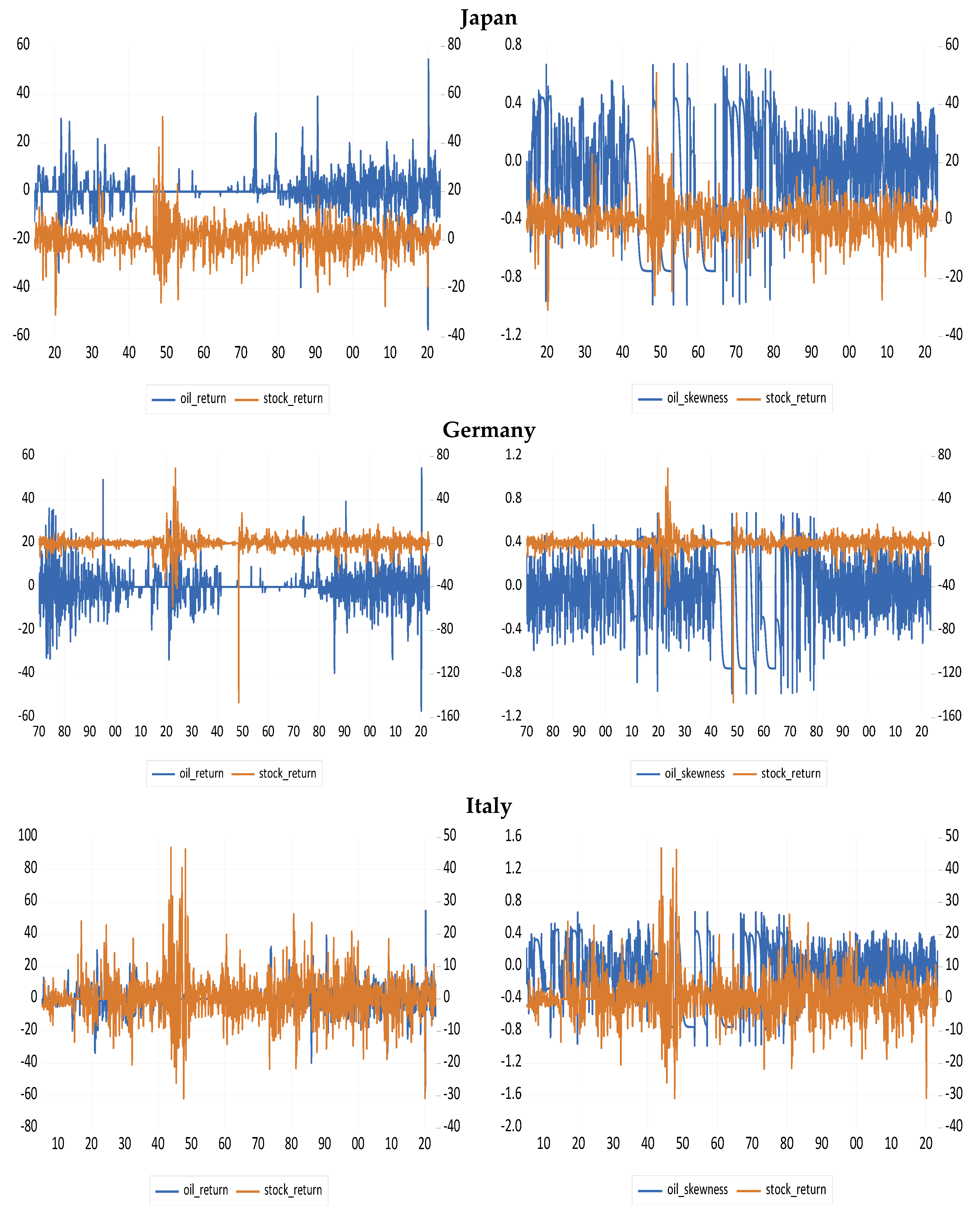
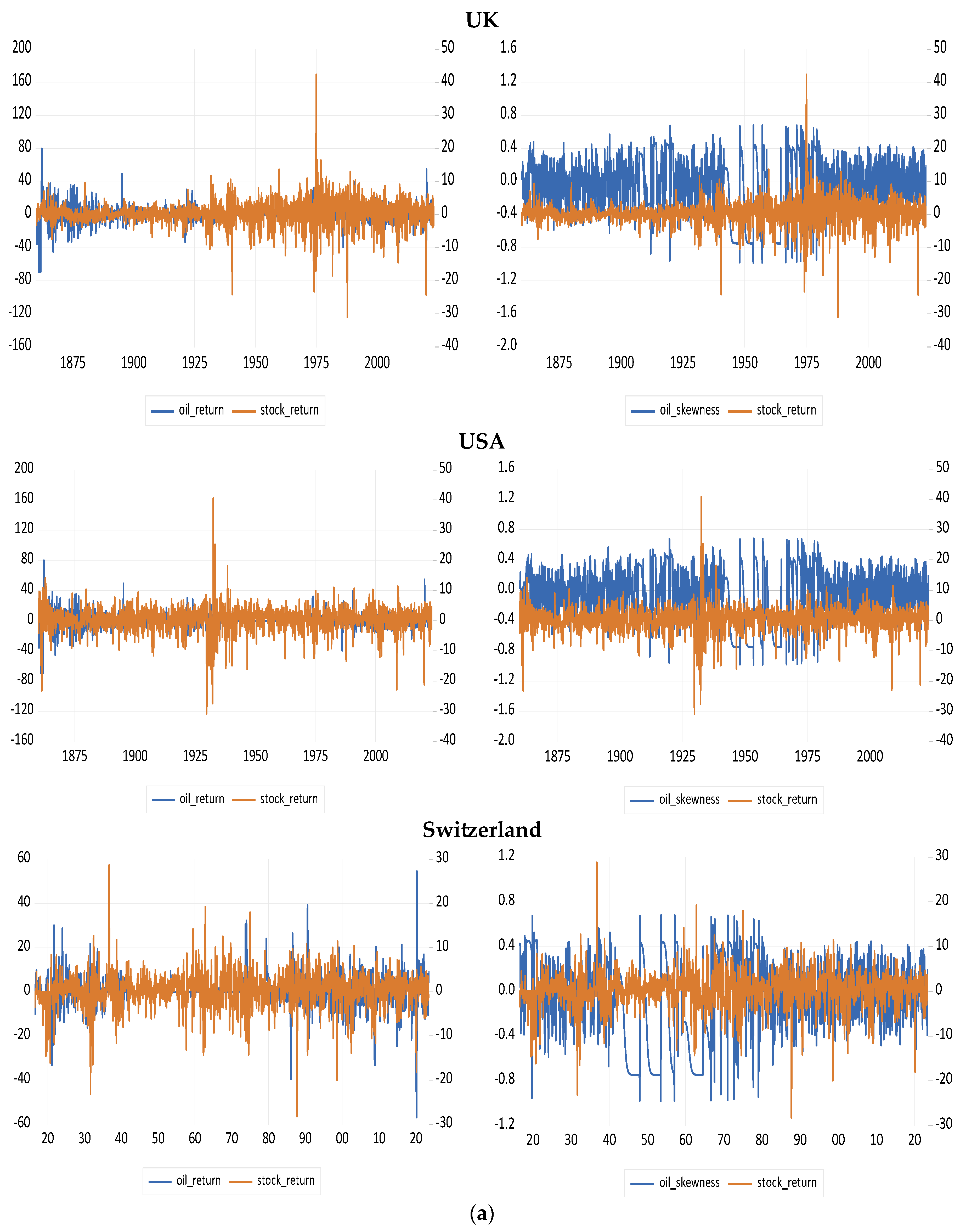
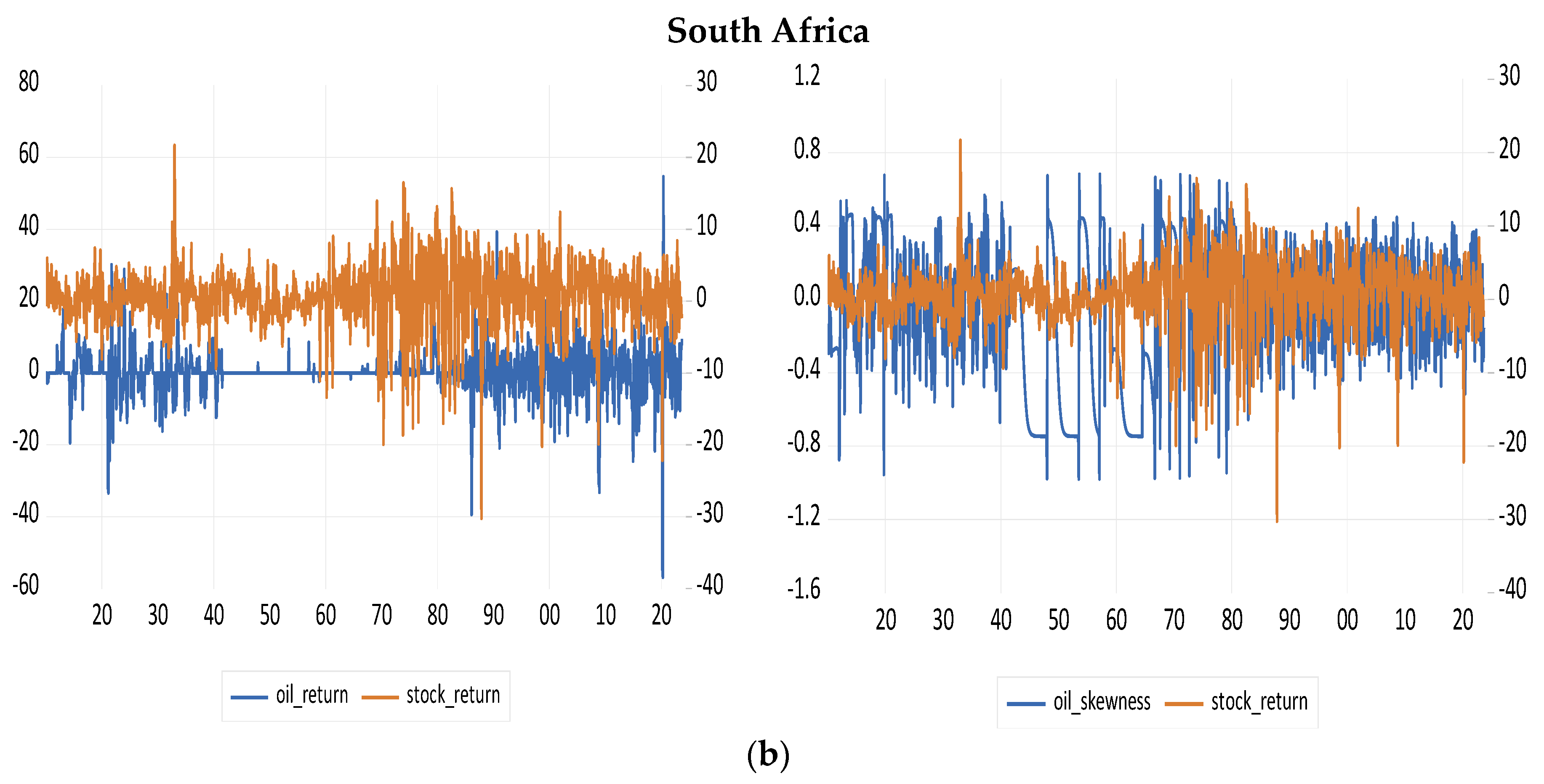
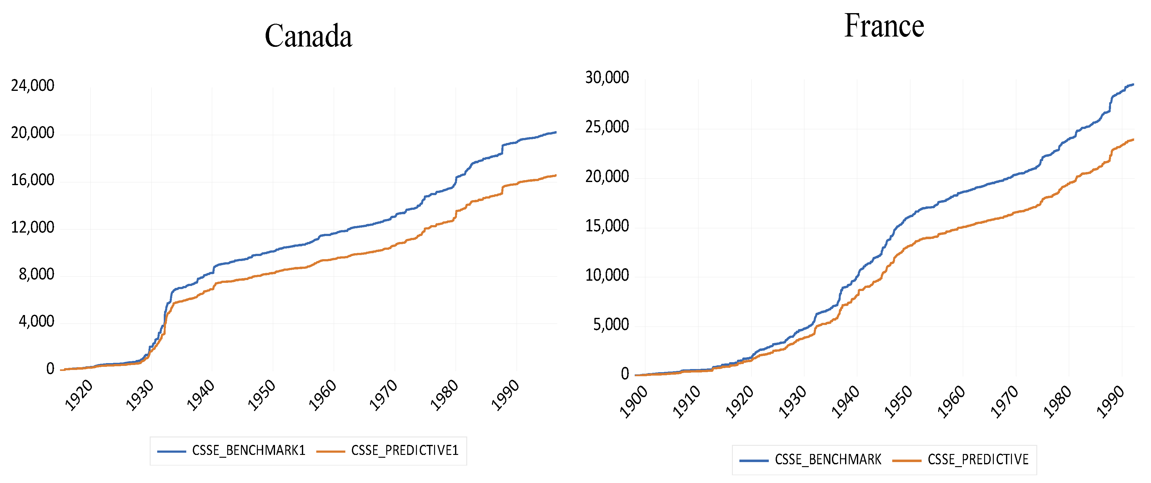
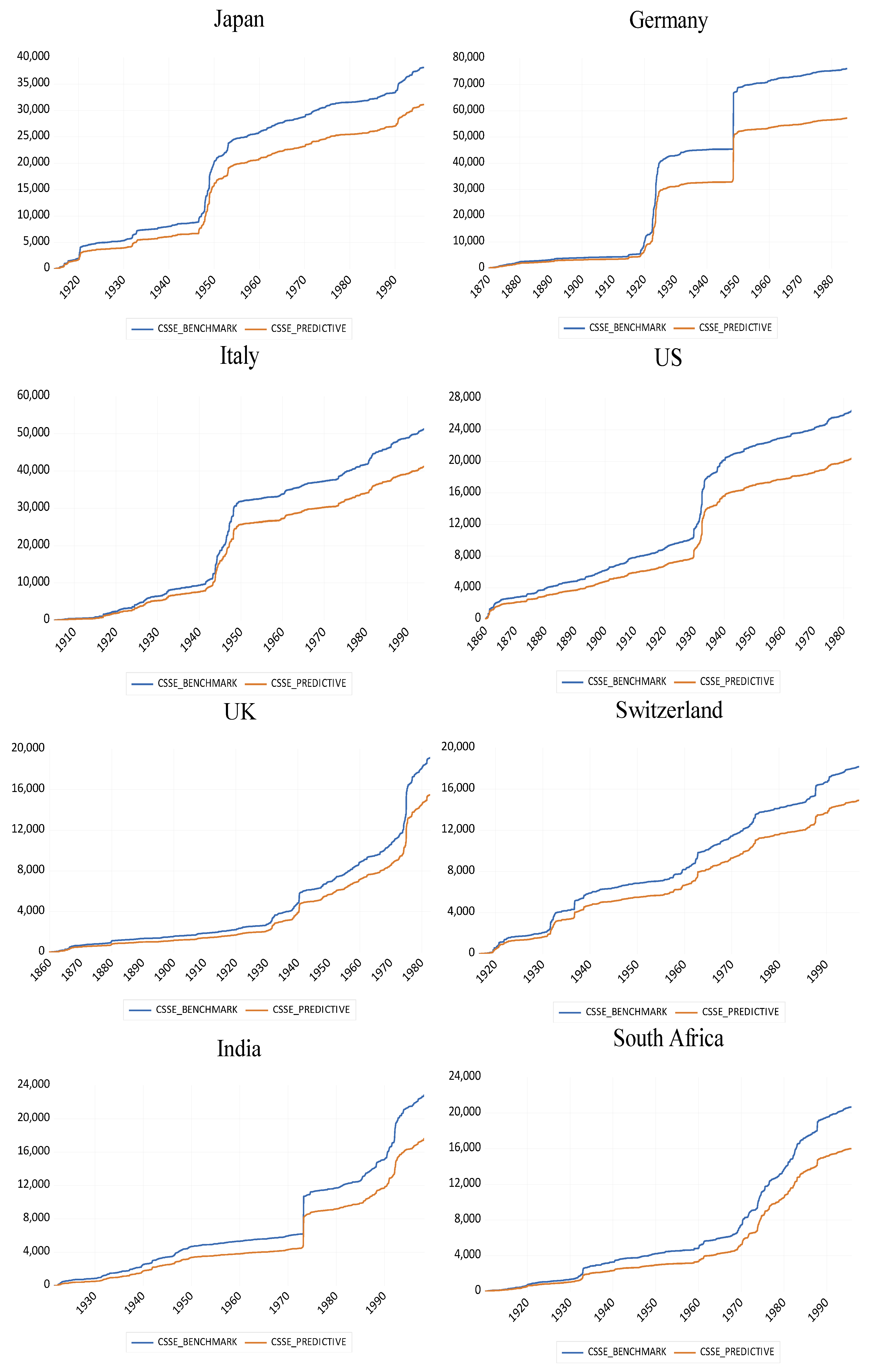
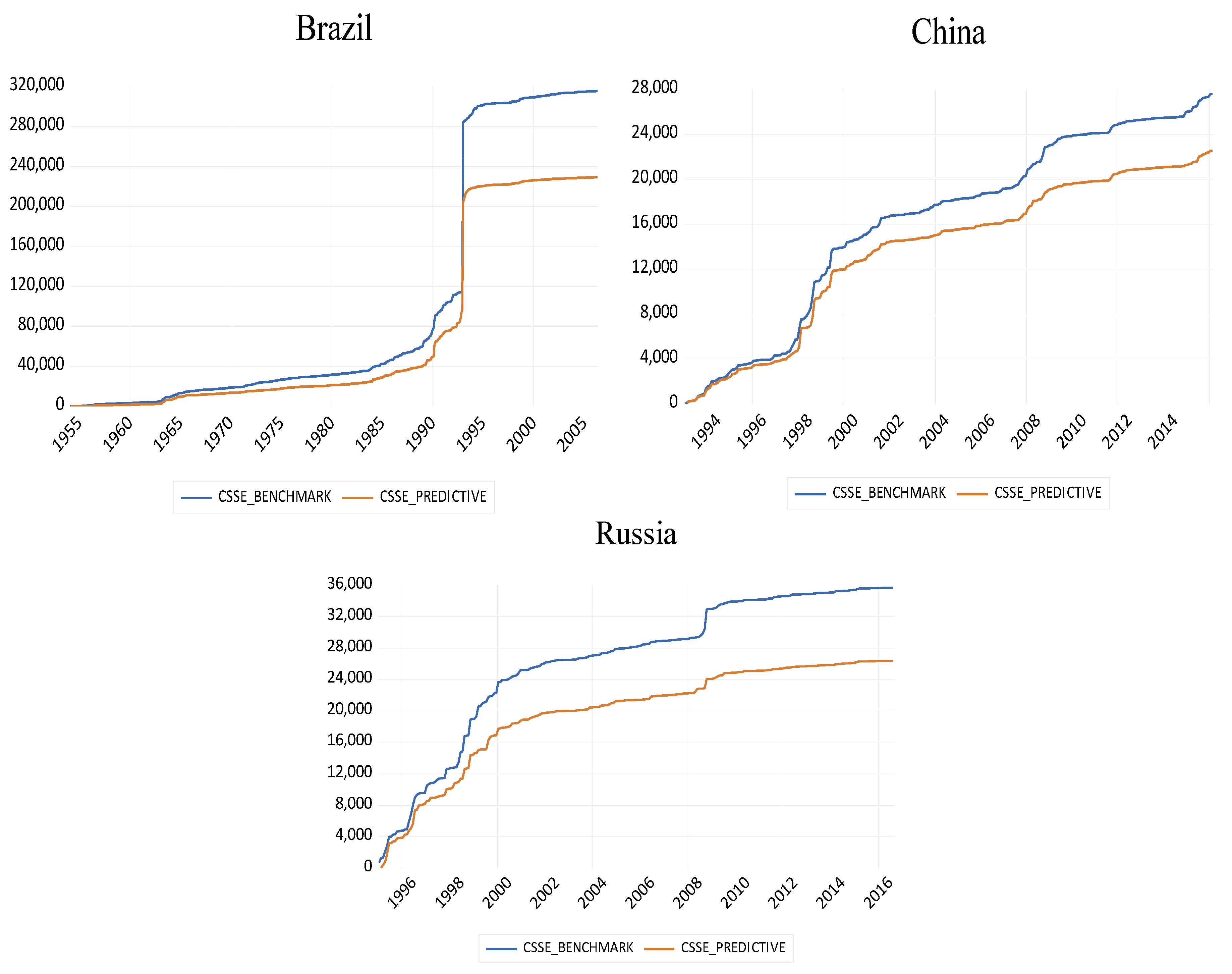
| 5 | The plots are based on a one-month ahead rolling window framework. The other forecast horizons (h = 3 and h = 6) follow the same pattern and are therefore suppressed for brevity. |
| 6 | See History.com via https://www.history.com/topics/world-war-i. Accessed on 1 June 2023. |
| 7 | According to Federal Reserve (see https://www.federalreservehistory.org/essays/great-depression#). Accessed on 1 June 2023. |
| 8 | See History.com via https://www.history.com/topics/world-war-ii. Accessed on 1 June 2023. |
| 9 | https://www.opec.org/opec_web/en/about_us/24.htm#. Accessed on 1 June 2023. |
| 10 | https://www.cdc.gov/museum/timeline/covid19.html. Accessed on 1 June 2023. |
| 11 | https://commonslibrary.parliament.uk/research-briefings/cbp-9847/. Accessed on 1 June 2023. |
References
- Balcilar, Mehmet, Rangan Gupta, and Christian Pierdzioch. 2022. Oil-price uncertainty and international stock returns: Dissecting quantile-based predictability and spillover effects using more than a century of data. Energies 15: 8436. [Google Scholar] [CrossRef]
- Balcilar, Mehmet, Rangan Gupta, and Mark E. Wohar. 2017. Common cycles and common trends in the stock and oil markets: Evidence from more than 150 years of data. Energy Economics 61: 72–86. [Google Scholar] [CrossRef]
- Balcilar, Mehmet, Rıza Demirer, and Shawkat Hammoudeh. 2019. Quantile relationship between oil and stock returns: Evidence from emerging and frontier stock markets. Energy Policy 134: 110931. [Google Scholar] [CrossRef]
- Balcilar, Mehmet, Rangan Gupta, and Stephen M. Miller. 2015. Regime switching model of US crude oil and stock market prices: 1859 to 2013. Energy Economics 49: 317–27. [Google Scholar] [CrossRef]
- Basher, Syed Abul, Alfred A. Haug, and Perry Sadorsky. 2018. The impact of oil-market shocks on stock returns in major oil-exporting countries. Journal of International Money and Finance 86: 264–80. [Google Scholar] [CrossRef]
- Bernanke, Ben. 2016. The relationship between stocks and oil prices. Ben Bernanke’s Blog on Brookings, February 19. [Google Scholar]
- Clark, Todd E., and Kenneth D. West. 2007. Approximately normal tests for equal predictive accuracy in nested models. Journal of Econometrics 138: 291–311. [Google Scholar] [CrossRef]
- Dai, Zhifeng, Huiting Zhou, Jie Kang, and Fenghua Wen. 2021. The skewness of oil price returns and equity premium predictability. Energy Economics 94: 105069. [Google Scholar] [CrossRef]
- Degiannakis, Stavros, George Filis, and Vipin Arora. 2018. Oil Prices and Stock Markets: A Review of the Theory and Empirical Evidence. The Energy Journal 39: 85–130. [Google Scholar] [CrossRef]
- Ebrahimi, Nima, and Craig Pirrong. 2018. The Risk of Skewness and Kurtosis in Oil Market and the Cross-Section of Stock Returns. Available online: https://ssrn.com/abstract=3168191 (accessed on 1 June 2023). [CrossRef]
- Engle, Robert F., and Simone Manganelli. 2004. CAViaR: Conditional Autoregressive Value at Risk by Regression Quantiles. Journal of Business & Economic Statistics 22: 367–81. [Google Scholar]
- Fernandez-Perez, Adrian, Bart Frijns, Ana-Maria Fuertes, and Joëlle Miffre. 2018. The Skewness of commodity futures returns. Journal of Banking and Finance 86: 143–58. [Google Scholar] [CrossRef]
- Galbraith, John Kenneth. 1990. A Short History of Financial Euphoria. New York: Penguin Books. [Google Scholar]
- Gupta, Rangan, and Mark Wohar. 2017. Forecasting oil and stock returns with a Qual VAR using over 150 years of data. Energy Economics 62: 181–86. [Google Scholar] [CrossRef]
- Gupta, Rangan, Florian Huber, and Philipp Piribauer. 2020. Predicting international equity returns: Evidence from time-varying parameter vector autoregressive models. International Review of Financial Analysis 68: 101456. [Google Scholar] [CrossRef]
- Gupta, Rangan, Qiang Ji, Christian Pierdzioch, and Vasilios Plakandaras. 2023. Forecasting the conditional distribution of realized volatility of oil price returns: The role of skewness over 1859 to 2023. Finance Research Letters 58: 104501. [Google Scholar] [CrossRef]
- Hamilton, James D. 2013. Historical Oil Shocks. In Routledge Handbook of Major Events in Economic History. Edited by Randall E. Parker and Robert Whaples. New York: Routledge Taylor and Francis Group, pp. 239–65. [Google Scholar]
- Hashmi, Shabir Mohsin, Bisharat Hussain Chang, and Niaz Ahmed Bhutto. 2021. Asymmetric effect of oil prices on stock market prices: New evidence from oil-exporting and oil-importing countries. Resources Policy 70: 101946. [Google Scholar] [CrossRef]
- Hodrick, Robert, and Edward C. Prescott. 1997. Postwar U.S. Business Cycles: An Empirical Investigation. Journal of Money, Credit, and Banking 29: 1–16. [Google Scholar]
- Ji, Qiang, Bing-Yue Liu, and Ying Fan. 2019. Risk dependence of CoVaR and structural change between oil international stock markets. Energy Economics 38: 136–45. [Google Scholar]
- Kelley, Truman L. 1947. Fundamentals of Statistics. Harvard: Harvard University Press. [Google Scholar]
- Kilian, Lutz, and Cheolbeom Park. 2009. The impact of oil price shocks on the US stock market. International Economic Review 50: 1267–87. [Google Scholar] [CrossRef]
- Ma, Yan-Ran, Dayong Zhang, Qiang Ji, and Jiaofeng Pan. 2019. Spillovers between oil and stock returns in the US energy sector: Does idiosyncratic information matter? Energy Economics 81: 536–44. [Google Scholar] [CrossRef]
- Mo, Xuan, Zhi Su, and Libo Yin. 2019. Can the skewness of oil returns affect stock returns? Evidence from China’s A-Share markets. North American Journal of Economics and Finance 50: 101042. [Google Scholar] [CrossRef]
- Narayan, Paresh Kumar, and Rangan Gupta. 2015. Has oil price predicted stock returns for over a century? Energy Economics 48: 18–23. [Google Scholar] [CrossRef]
- Pan, Lei, and Vinod Mishra. 2022. International portfolio diversification possibilities: Can BRICS become a destination for US investors? Applied Economics 54: 2302–19. [Google Scholar] [CrossRef]
- Rapach, David, and Guofu Zhou. 2013. Forecasting stock returns. In Handbook of Economic Forecasting. Edited by Graham Elliott and Allan Timmermann. Amsterdam: Elsevier, vol. 2 (Part A), pp. 328–83. [Google Scholar]
- Rapach, David, and Guofu Zhou. 2022. Asset Pricing: Time-Series Predictability. Oxford Research Encyclopedia of Economics and Finance. Available online: https://oxfordre.com/economics (accessed on 1 June 2023).
- Reinhart, Carmen M., and Kenneth S. Rogoff. 2009. This Time Is Different: Eight Centuries of Financial Folly. Princeton: Princeton University Press. [Google Scholar]
- Reinhart, Carmen M., and Kenneth S. Rogoff. 2011. From Financial Crash to Debt Crisis. American Economic Review 101: 1676–706. [Google Scholar] [CrossRef]
- Reinhart, Carmen M., and Vincent R. Reinhart. 2010. After the fall. Paper presented at the Economic Policy Symposium, Jackson Hole, Federal Reserve Bank of Kansas City, Jackson Hole, WY, USA, August 26–28; pp. 17–60. [Google Scholar]
- Salisu, Afees A., Abeeb O. Olaniran, and Xuan Vinh Vo. 2023. Tail risks and forecastability of stock returns of advanced economies: Evidence from centuries of data. The European Journal of Finance 29: 466–81. [Google Scholar] [CrossRef]
- Salisu, Afees A., Abeeb O. Olaniran, and Xuan Vinh Vo. 2025. Geopolitical Risk, Climate Risk and Financial Innovation in the Energy Market. Energy 2025: 134365. [Google Scholar] [CrossRef]
- Salisu, Afees A., and Rangan Gupta. 2022. Commodity Prices and Forecastability of International Stock Returns over a Century: Sentiments versus Fundamentals with Focus on South Africa. Emerging Markets Finance and Trade 58: 2620–36. [Google Scholar] [CrossRef]
- Salisu, Afees A., Rangan Gupta, and Riza Demirer. 2022. Oil Price Uncertainty Shocks and Global Equity Markets: Evidence from a GVAR Model. Journal of Risk and Financial Management 15: 355. [Google Scholar] [CrossRef]
- Sheng, Xin, Rangan Gupta, and Qiang Ji. 2023. The Effects of Disaggregate Oil Shocks on Aggregate Expected Skewness of the United States. Risks 11: 186. [Google Scholar] [CrossRef]
- Smyth, Russell, and Paresh Kumar Narayan. 2018. What do we know about oil prices and stock returns? International Review of Financial Analysis 57: 148–56. [Google Scholar] [CrossRef]
- Stock, James H., and Mark W. Watson. 2003. Forecasting Output and Inflation: The Role of Asset Prices. Journal of Economic Literature 41: 788–829. [Google Scholar] [CrossRef]
- Tavor, Tchai. 2024. Assessing the financial impacts of significant wildfires on US capital markets: Sectoral analysis. Empirical Economics 67: 1115–48. [Google Scholar] [CrossRef]
- Wang, Yudong, Zhiyuan Pan, Li Liu, and Chongfeng Wu. 2019. Oil price increases and the predictability of equity premium. Journal of Banking and Finance 102: 43–58. [Google Scholar] [CrossRef]
- Welch, Ivo, and Amit Goyal. 2008. A comprehensive look at the empirical performance of equity premium prediction. The Review of Financial Studies 21: 1455–508. [Google Scholar] [CrossRef]
- Westerlund, Joakim, and Paresh Kumar Narayan. 2012. Does the choice of estimator matter when forecasting returns? Journal of Banking & Finance 36: 2632–40. [Google Scholar]
- Westerlund, Joakim, and Paresh Kumar Narayan. 2015. Testing for predictability in conditionally heteroscedastic stock returns. Journal of Financial Econometrics 13: 342–75. [Google Scholar] [CrossRef]
- Yin, Libo, and Yang Wang. 2019. Forecasting the oil prices: What is the role of skewness risk? Physica A: Statistical Mechanics and Its Applications 534: 120600. [Google Scholar] [CrossRef]
| Country | |||
|---|---|---|---|
| Canada | 8.749 *** [1.294] | 8.730 *** [1.290] | 8.676 *** [1.285] |
| France | 9.085 *** [0.931] | 9.084 *** [0.928] | 9.062 *** [0.925] |
| Japan | 15.151 *** [2.710] | 15.128 *** [2.702] | 15.030 *** [2.690] |
| Germany | 24.507 *** [5.041] | 24.452 *** [5.030] | 24.373 *** [5.014] |
| Italy | 20.587 *** [3.582] | 20.559 *** [3.572] | 20.424 *** [3.559] |
| US | 9.491 *** [1.064] | 9.537 *** [1.062] | 9.536 *** [1.059] |
| UK | 2.266 *** [0.294] | 2.279 *** [0.294] | 2.265 *** [0.294] |
| Switzerland | 7.931 *** [1.156] | 7.989 *** [1.154] | 7.953 *** [1.150] |
| India | 5.378 *** [0.503] | 5.341 *** [0.502] | 5.319 *** [0.500] |
| South Africa | 4.882 *** [0.578] | 4.871 *** [0.577] | 4.850 *** [0.575] |
| Country | |||
|---|---|---|---|
| Canada | 8.073 *** [0.932] | 8.113 *** [0.931] | 8.093 *** [0.928] |
| France | 9.661 *** [0.836] | 9.690 *** [0.835] | 9.677 *** [0.833] |
| Japan | 12.754 *** [1.860] | 12.716 *** [1.857] | 12.734 *** [1.852] |
| Germany | 25.356 *** [5.656] | 25.327 *** [5.648] | 25.457 *** [5.636] |
| Italy | 19.393 *** [2.500] | 19.414 *** [2.496] | 19.353 *** [2.489] |
| US | 8.156 *** [0.747] | 8.166 *** [0.746] | 8.184 *** [0.745] |
| UK | 4.731 *** [0.615] | 4.734 *** [0.615] | 4.749 *** [0.613] |
| Switzerland | 7.465 *** [0.876] | 7.511 *** [0.875] | 7.637 *** [0.876] |
| India | 11.455 *** [1.738] | 11.583 *** [1.738] | 11.602 *** [1.733] |
| South Africa | 8.686 *** [0.835] | 8.711 *** [0.834] | 8.684 *** [0.832] |
| Panel A: 50–50%–Split | |||
| Country | |||
| Brazil | 89.049 *** [11.790] | 101.046 *** [14.810] | 107.183 *** [15.543] |
| China | 14.467 *** [4.120] | 14.326 *** [4.081] | 14.051 *** [4.025] |
| Russia | 26.248 *** [10.590] | 26.024 *** [10.481] | 25.398 *** [10.332] |
| Panel B: 75–25%-Split | |||
| Country | |||
| Brazil | 326.514 *** [108.257] | 325.859 *** [107.913] | 324.538 *** [107.403] |
| China | 10.758 *** [2.826] | 10.685 *** [2.807] | 10.602 *** [2.779] |
| Russia | 17.548 *** [6.665] | 17.416 *** [6.6175] | 17.275 *** [6.548] |
Disclaimer/Publisher’s Note: The statements, opinions and data contained in all publications are solely those of the individual author(s) and contributor(s) and not of MDPI and/or the editor(s). MDPI and/or the editor(s) disclaim responsibility for any injury to people or property resulting from any ideas, methods, instructions or products referred to in the content. |
© 2025 by the authors. Licensee MDPI, Basel, Switzerland. This article is an open access article distributed under the terms and conditions of the Creative Commons Attribution (CC BY) license (https://creativecommons.org/licenses/by/4.0/).
Share and Cite
Salisu, A.A.; Gupta, R. Commodity Risk and Forecastability of International Stock Returns: The Role of Oil Returns Skewness. Risks 2025, 13, 49. https://doi.org/10.3390/risks13030049
Salisu AA, Gupta R. Commodity Risk and Forecastability of International Stock Returns: The Role of Oil Returns Skewness. Risks. 2025; 13(3):49. https://doi.org/10.3390/risks13030049
Chicago/Turabian StyleSalisu, Afees A., and Rangan Gupta. 2025. "Commodity Risk and Forecastability of International Stock Returns: The Role of Oil Returns Skewness" Risks 13, no. 3: 49. https://doi.org/10.3390/risks13030049
APA StyleSalisu, A. A., & Gupta, R. (2025). Commodity Risk and Forecastability of International Stock Returns: The Role of Oil Returns Skewness. Risks, 13(3), 49. https://doi.org/10.3390/risks13030049