Relationship Between Japanese Stock Market Behavior and Category-Based News

Abstract

This study investigates the relationship between news delivered via the QUICK terminal and stock market behavior. Specifically, through an evaluation of the performance of investment strategies that utilize news index created based on its scores indicating positive or negative sentiment, we examine whether index construction that takes into account the content of individual news items contributes to improved predictive power with regard to stock prices. We verify the performance of this investment strategy based on signal indicators derived from news indices focusing on short-term trends using time-series decomposition. After refining the news indicators based on news categories, we observe an improvement in the strategy’s performance, demonstrating that the value of news varies across different categories and the importance of considering the content and meaning of text news.

1. Introduction

In recent years, there has been a growing trend of analyzing text information, such as news, to better understand market activities. Numerous studies have investigated methods for mechanically scoring text information, and various applications have been used to make predictions in financial markets (e.g., Bollen et al. 2011; Boudoukh et al. 2012; Lee et al. 2014; Li et al. 2019; Narayan and Bannigidadmath 2017; Schumaker and Chen 2009). However, diverse and differing results have been reported, suggesting that a universal generalized method for market prediction has yet to be established. Meanwhile, to our knowledge, there has been little research conducted on predictability under conditions that consider the classification of text news. Therefore, what we want to clarify with this study, using performance as an investment strategy, is whether or not considering specific categories in the news improves the predictive power of the news for stock prices.

To accurately understand the current state of market prediction through news scoring, we use data analysis to investigate the relationship between news text, its mechanical scoring results, and stock trading outcomes in the market. Specifically, based on the hypothesis that news scoring’s effect on market prediction accuracy varies significantly by news category, we use exploratory data analysis (EDA)1 to confirm the existence of news categories where mechanical scoring is more effective for predictions. To verify the existence of news categories suitable for predictions, we prepare news indices based on the entire news dataset, as per Tetlock (2007), and indices focused on categories deemed suitable for predictions. We then devise investment strategies using these indices and compare their respective investment performances.

Regarding prior research on the relationship between news and stock markets, Tetlock (2007) used a news index based on Wall Street Journal articles to validate information theory. Information theory was validated in that study using a three-variable vector autoregressive model based on news indices, stock returns, and trading volume. That study found that the occurrence of pessimistic language in market observation column articles temporarily affects subsequent returns in the US stock market. However, stock prices tend to rebound and negate these short-term effects, leading us to conclude that there is limited evidence supporting the idea that text-based information fundamentally influences stock prices. Roll (1988) likewise expressed skepticism regarding the effect of news on stock prices. Specifically, using the monthly returns of US-listed stocks, the author found that news had minimal explanatory power for individual stock or industry-level returns, as indicated by low R² values.

Boudoukh et al. (2012), however, provided evidence for the effect of news information on stock prices in the US. They considered the tone (positive or negative) of the news content and measured its effect on US stock prices. Contrary to Roll (1988), they argued that news indices incorporating tone considerations can partially explain stock prices, as confirmed by R² values. Tetlock (2011) also adopted a unique approach by leveraging the similarity across multiple news articles to examine investor behavior. That study assessed the novelty of news by calculating word occurrence rates in the news using text mining techniques. Notably, the findings revealed that individual investors often trade without distinguishing between new and previously reported news. Furthermore, Tetlock et al. (2008) used simple indices derived from the news to examine the predictability of individual company earnings and stock performance. Their findings suggested that the proportion of negative words in the news could help predict poor company performance. Meanwhile, Okimoto and Hirasawa (2014) applied a similar method to that of Tetlock (2007) to Japanese stocks. They confirmed that news indices created based on news distributed via the QUICK terminal2 had significant explanatory power for the next day’s returns on Japanese stocks. This finding suggests that the news holds intrinsic information relevant to stock prices.

Aside from research focusing on developed economies such as the US and Japan, studies have examined the influence and predictability of textual information for stock markets in broader contexts. Narayan and Bannigidadmath (2017) and Shen et al. (2022) both tested the predictability of the stock market using news data, each in an ingenious way. Narayan and Bannigidadmath (2017) examined Islamic stocks, while Shen et al. (2022) examined Chinese stocks; both studies concluded that news data had predictive power for the stock market under investigation.

While relatively few studies have delved into the interpretation of news content, Bybee et al. (2023) considered the meaning of news as topics in their topic model. Specifically, using a topic model that summarized Wall Street Journal articles into comprehensible themes (Bybee et al. 2021), Bybee et al. (2023) constructed a factor model based on textual information to demonstrate its effectiveness. A notable feature of that study was the extraction of topics using unsupervised machine learning, which captured the diversity of contexts by retrospectively assigning meanings to topics based on the analyst’s perspective. Our study, by contrast, uses widely recognized article categories as they are, thereby eliminating the subjective analyst bias often encountered in the handling of topic models.

Through a study on the use of news topics to measure stock market sentiment, Uhl and Novacek (2020) showed the effectiveness of dynamically selecting news data for predicting stock market returns and proposed a new method for constructing sentiment indices based on correlation coefficients with stock index returns. The study showed that top news sentiment, which is calculated only for a topic with the highest correlation to equity indices, has robust predictive power in the US stock market and that investment strategies based on it work effectively. While their study selected topics with daily global news topics, our analysis is based on more detailed news categories related to the Japanese stock market. Although the granularity of news categorization is different, there is a similarity in examining news content, and selecting appropriate categories can lead to improved effectiveness. A comparison of the characteristics and main results of their study and ours will be discussed in detail in Section 6.

Zhang (2006) conducted a study to investigate the impact of the news on stock prices from the perspective of information uncertainty in the US stock market. The study showed that information uncertainty affects the speed with which investors react to new information, which plays an important role in predicting stock returns. The study suggests that this investor behavioral bias is amplified by information uncertainty and that greater information uncertainty leads to greater price drift, resulting in higher expected returns following good news and lower expected returns following bad news. Zhang (2006) defined good or bad news in terms of analysts’ earnings forecast revisions, which are associated with a specific news category in the news in our study. Its results are consistent with our analysis, and a comparison with our analysis will be made in detail in Section 3.

Building on previous studies, we use EDA to examine the effect of news scoring on predictions of the Japanese stock market, particularly differences in stock performance by news category. In other words, we test the predictive validity of news data by category using a means of measuring market sentiment with news data, as proposed by Tetlock (2007) and demonstrated by Okimoto and Hirasawa (2014), whose method is commonly used for Japanese news data. Furthermore, we create new news indices reflecting differences in the value of news by category, as discovered through EDA, and examine changes in their performance. In almost all previous studies examining the predictive nature of news data, such as those listed above, all available news data are used without interpreting their meaning. Failing to consider the content and meaning of news articles might result in unnecessary noise affecting the predictive power of the stock market. By contrast, the major motivation and main contribution of our study is that we not only show that different categories of news articles have different effects on the stock market but also imply that news indices that consider the meaning of news articles are of superior quality to news indices that use all news data available without consideration in terms of their predictive power for the stock market.

The next section outlines the objectives of our study. Then, Section 3 describes the news data used in this study and their characteristics, as well as the preliminary findings, which are the results of the EDA conducted for each news category. Section 4 explains the data analysis method used to verify the presence or absence of category effects in news scoring’s effect on Japanese stock market prediction; we also provide an overview of our investment strategy using news data. Section 5 presents the main results, which are then discussed in Section 6. Section 7 provides the conclusions of this study.

2. Objective of This Study

The objective of this study is to clarify the relationship between the news and stock market behavior. In particular, we confirm that the news also has predictive power for stock returns in the Japanese market, as recent studies have shown, and we show that an effective selection of news categories exists, which can improve predictive power for Japanese stock returns.

In order to gain insight into the relationship between news categories and stock returns and to suggest what news categories should be selected, we first conducted EDA to analyze the performance in stock prices after news distribution for each individual category. To our knowledge, few studies have examined the contribution of the news categories to the predictive power for the stock market.

Thus, the goal of our study is to confirm that investment strategies using the news index proposed in the previous research still have the power to predict stock returns in the Japanese stock market; we also aim to show that a suitable news category selection method can improve the performance of the investment strategy.

3. Data and Preliminary Findings

Our analysis uses news data from the QUICK terminal distributed from 1 December 2010 to 15 April 2022. The dataset comprises over three million news articles delivered via the QUICK terminal, covering 4234 domestically listed companies. Since the QUICK terminal is widely accessed by Japanese market participants in real time, it is a highly influential source of market information.

The QUICK news data3 include essential information such as timestamps indicating when the article was delivered, target stock names, and event details related to the news content. The data also incorporate scores denoting positive or negative sentiment, generated using proprietary big data analytics technology developed by Nikkei Financial Technology Research Institute. These sentiment scores are quantified based on natural language processing and proprietary estimation rules. A score closer to 0 indicates a negative market reaction, while a score closer to 100 suggests a positive reaction. Leveraging these sentiment scores, we examine the correlation between our news indices and stock market indices and propose investment strategies based on news indices. The average score in our news data is 51.2, with a median of 48 and an unbiased standard deviation of 25.1. We categorize news as positive if the score exceeds 50 and negative if it falls below 50. In terms of creating our news indices, news data with a score precisely equal to 50 are excluded from the news index calculation.

Table 1. Statistics for the top five events by the number of news items delivered. The mean, median, maximum, and minimum of sentiment scores are shown for the corresponding news items. SD indicates standard deviation.

No.	Events	Average	Median	Max	Min	SD	Skewness	Kurtosis
1	Market Rise	66.0	50	99	14	20.8	0.6	−1.7
2	Market Decline	36.2	50	85	1	20	−0.8	−1.4
3	Increase in Large-Volume Holdings	49.7	50	96	11	10.1	1.2	3.5
4	Decrease in Large-Volume Holdings	39.6	39	86	13	5.4	0.9	3.3
5	Rise in Stock Rating	79.8	84	84	4	13.2	−1.4	1.0

presents statistical values for the scores of the top five events representing news content. Notably, the delivered news exhibits a mix of information related to past market events (e.g., “Market Rise” or “Market Decline”) and news concerning changes in holdings by major investors (e.g., “Increase in Large-Volume Holdings” or “Decrease in Large-Volume Holdings”).

Figure 1 illustrates the distribution of news occurrence times for all analyzed news. Notably, news delivery occurs most frequently during the trading hours of the Tokyo Stock Exchange (09:00–15:00), with the maximum number of deliveries occurring at market close (15:00). Post-market hours see a gradual decrease in news postings. It is practically impossible to execute stock trades based on news delivered at precisely 15:00. Therefore, when proposing investment strategies using such news sources, it is important to distinguish between news delivered during trading hours and outside trading hours, as we did in this study. The TOPIX (Tokyo Stock Price Index), which we used as our investment objective in this study, is a market capitalization-weighted equity index of Japanese stocks and is a major equity index that is used as a benchmark for the Japanese stock market. The TOPIX and TOPIX futures data we used in this study were obtained from Bloomberg, while individual stock price data were sourced from the QUICK terminal.

3.1. Relationship Between News Data and Stock Performance

To further understand the relationship between news content and subsequent stock price performance, we examine the average excess returns against the TOPIX immediately after news delivery. The following subsections explain the analysis of their relationships, their implications, and the effects of each company’s market capitalization.

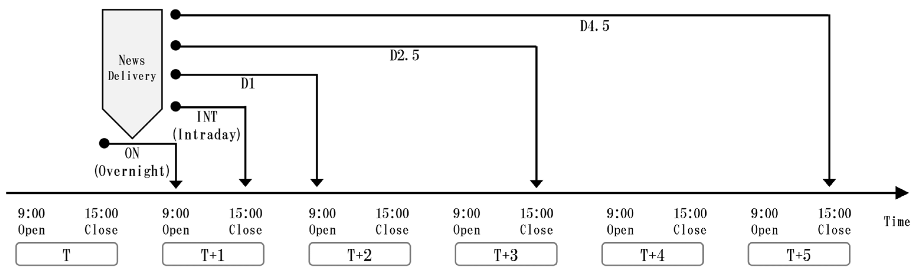
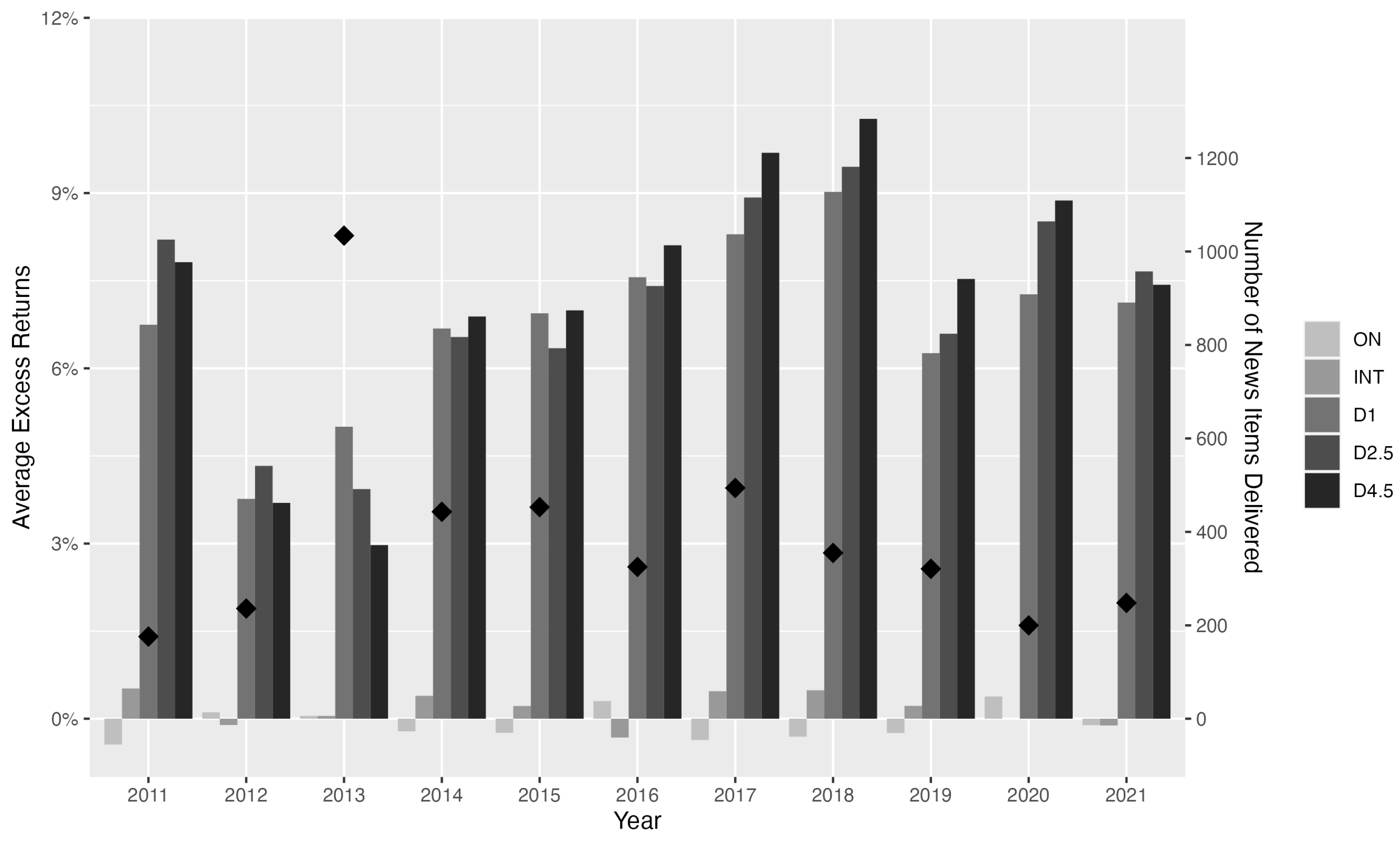
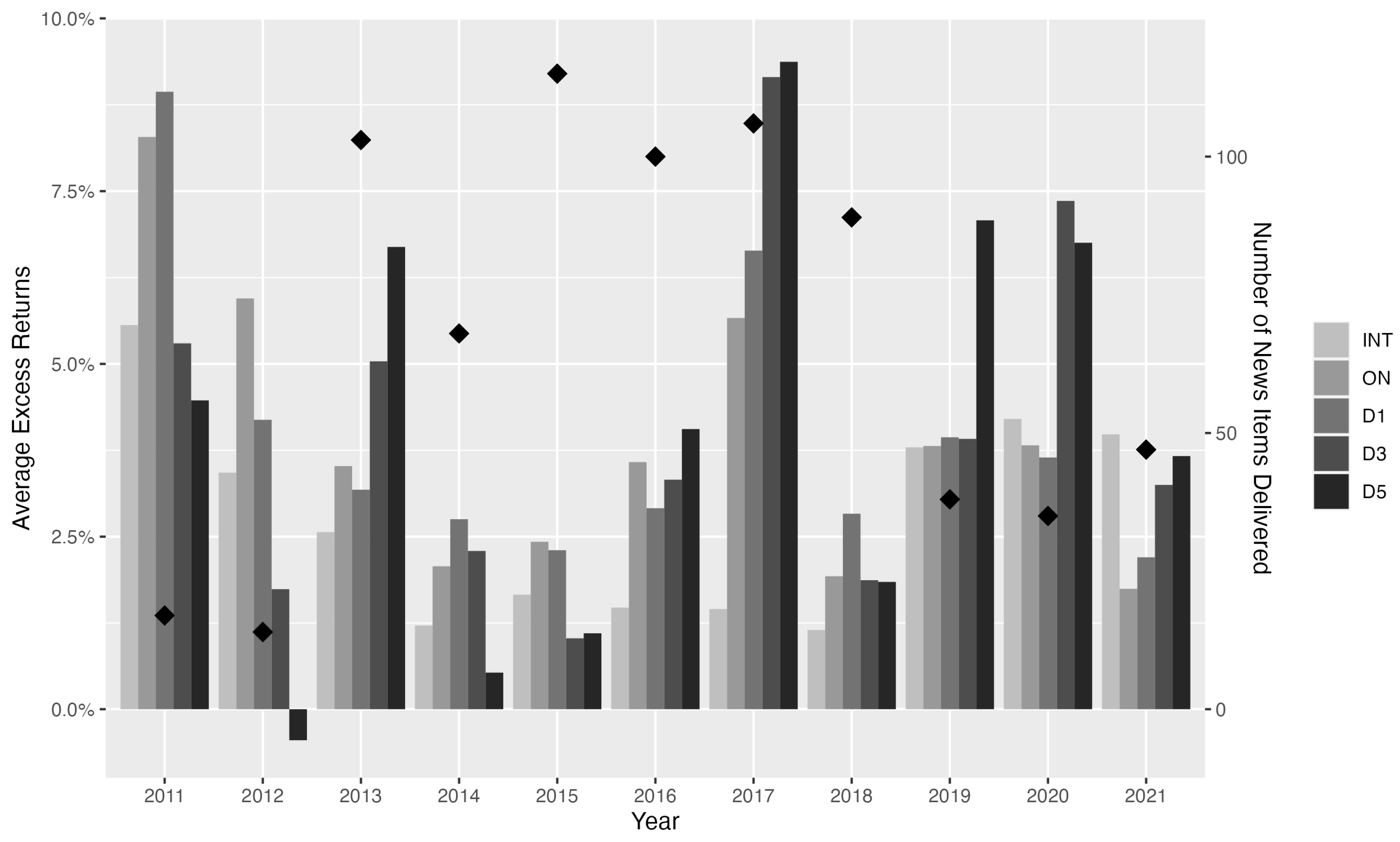
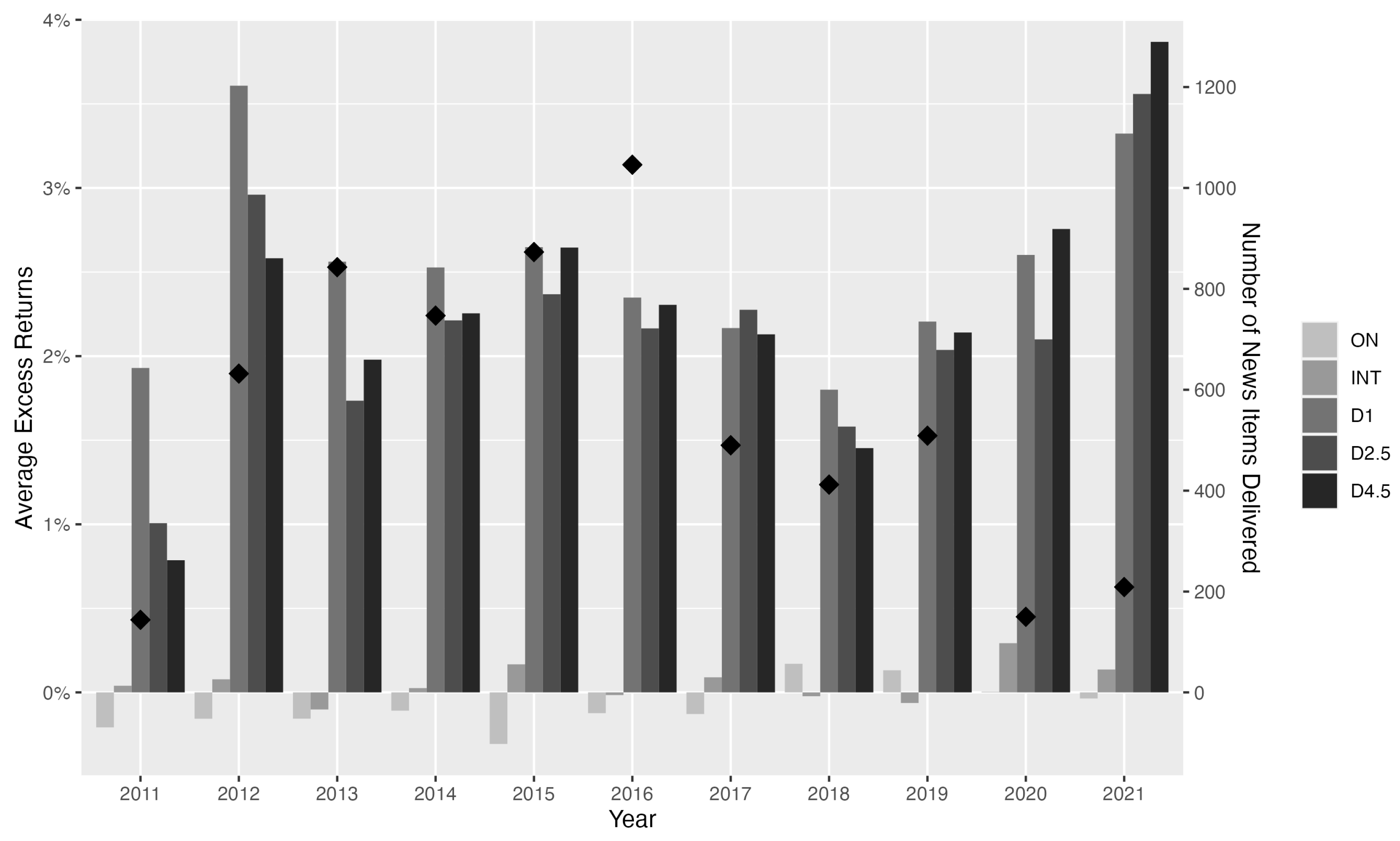
3.1.1. Average Excess Returns for News by Events and Score

First, we examine the average excess returns against the TOPIX immediately after news delivery for the top 30 events, represented by their news tags.

Table 2. Stock performance by event for news delivered during trading hours. This presents the excess returns relative to the TOPIX for each event for news delivered during trading hours, considering different time horizons.

No.	News Tag	Average Score	INT (%)	ON (%)	D1 (%)	D3 (%)	D5 (%)
1	Market Rise	83.3	1.1	1.3	1.0	1.0	0.9
2	Market Decline	18.2	−0.8	−0.8	−0.9	−1.1	−1.1
3	Increase in Large-Volume Holdings	49.6	0.1	0.1	0.1	0.1	0.1
4	Decrease in Large-Volume Holdings	39.4	−0.1	0.0	0.0	0.0	0.0
5	Sales Increase	55.1	0.0	0.1	0.1	0.1	0.1
6	Profit Increase	60.4	0.1	0.1	0.2	−0.1	−0.1
7	Rise in Stock Rating	82.5	0.2	0.5	0.6	0.7	0.9
8	Profit Increase: Market Rise	92.4	0.7	0.6	0.5	0.5	0.5
9	Sales Decrease	40.8	−0.1	0.0	0.0	0.0	−0.1
10	Profit Forecast Increase: Market Rise	93.4	0.8	1.1	0.9	0.9	0.9
11	Sales Increase: Market Rise	94.3	0.8	0.7	0.7	0.8	0.8
12	Profit Decrease	36.4	−0.2	−0.3	−0.4	−0.6	−0.6
13	Stock Rating Downgrade	13.9	−0.3	−0.4	−0.5	−0.7	−0.6
14	Missing QUICK Consensus Estimate	38.3	−0.2	−0.2	−0.3	−0.7	−0.7
15	Profit Forecast Decrease: Market Decline	6.0	−0.4	−0.9	−1.1	−1.4	−1.4
16	Profit Decrease: Market Decline	7.7	−0.6	−0.5	−0.5	−0.6	−0.6
17	Stock Rating Downgrade: Market Decline	5.8	−0.6	−0.6	−0.6	−0.6	−0.5
18	Profit Increase: Market Decline	9.6	−1.0	−0.6	−0.9	−1.3	−1.4
19	Scandal	43.1	−0.2	−0.8	−0.8	−1.2	−1.3
20	Buyback	83.3	1.7	0.9	0.9	0.9	1.0
21	Profit Forecast Increase	72.8	0.2	0.5	0.4	0.4	0.5
22	Market Rise: Sales Increase	91.3	1.1	1.1	1.1	1.2	1.0
23	Buyback: Market Rise	93.2	0.5	0.3	0.1	0.3	0.3
24	Exceeding QUICK Consensus Estimate	72.8	0.6	0.7	0.9	0.9	1.0
25	Stock Split	77.2	2.1	3.4	3.6	4.0	4.3
26	Profit Forecast Decrease	24.7	−0.1	−0.8	−1.0	−1.3	−1.1
27	Profit Decrease: Market Rise	89.4	1.0	1.0	0.9	0.8	0.6
28	Profit Forecast Decrease: Market Decline	10.9	−1.1	−0.6	−0.8	−1.1	−1.3
29	Falsehood and Disguise	43.8	0.1	−0.7	−0.8	−0.7	−0.5
30	Sales Increase: Sales Decrease	38.9	0.0	0.0	0.0	−0.3	−0.5

presents the excess returns relative to the TOPIX for each event for news delivered during trading hours, considering different time horizons. Specifically, it shows the overnight excess returns from the closing price to the opening price on the next business day (labeled ON), the excess returns from the closing price to the closing price on the next business day (D1), those from the closing price to the closing price three business days later (D3), and those from the closing price to the closing price five business days later (D5). Additionally, to examine the effect of the news on stock prices on the day of news delivery, the table shows the intraday excess return from the opening price to the closing price on the same day (labeled INT). In Figure 2, we graphically illustrate the measurement of performance, as explained above, in response to the news delivered during trading hours on day T. Figure 2 clarifies which day’s market open or which day’s market close is referred to by the stock performance.

As Table 2 shows, except for news conveying past realized stock price movements (“Market Rise” or “Market Decline”), events such as “Stock Split” and “Buyback” outperform the TOPIX, while events such as “Stock Rating Downgrade”, “Missing QUICK Consensus Estimate”, and “Scandal” show negative performance trends. Additionally, the momentum effect tends to persist even after the initial effect, especially for event No. 25, i.e., “Stock Split”.

Table 3. Stock performance by event for news delivered after market close. This presents the excess returns relative to the TOPIX for each event for news delivered after market close, considering different time horizons.

No.	News Tag	Average Score	ON (%)	INT (%)	D1 (%)	D2.5 (%)	D4.5 (%)
1	Rise in Stock Rating	80.3	−0.1	0.1	1.4	1.7	1.8
2	Increase in Large-Volume Holdings	49.9	0.0	0.0	0.3	0.4	0.4
3	Decrease in Large-Volume Holdings	39.1	0.1	−0.1	−0.2	−0.4	−0.6
4	Stock Rating Downgrade	20.9	0.1	−0.1	−1.0	−1.1	−1.2
5	Profit Increase	60.2	0.0	0.1	0.7	0.5	0.4
6	Sales Increase	53.7	−0.1	0.1	0.3	0.3	0.3
7	Profit Decrease	36.3	0.0	0.0	−0.6	−0.7	−0.7
8	Market Rise	61.0	−1.1	0.7	1.5	1.1	1.0
9	Sales Decrease	41.2	0.0	0.0	−0.2	−0.4	−0.5
10	Buyback	79.2	−0.1	0.0	2.6	2.2	2.3
11	Profit Increase: Sales Increase	64.0	−0.1	0.1	0.9	0.6	0.6
12	Missing QUICK Consensus Estimate	37.7	0.0	0.0	−0.5	−0.8	−0.9
13	Market Decline	38.8	1.1	−0.4	−1.4	−1.6	−1.7
14	Stock Split	87.7	−0.1	0.2	6.6	6.6	6.8
15	Increased Dividend	80.7	−0.4	0.4	3.6	3.1	3.0
16	Profit Forecast Increase	72.3	0.0	0.1	1.8	1.7	1.6
17	No or Reduced Dividend	21.4	0.1	0.0	−1.3	−1.9	−2.2
18	Profit Forecast Decrease	25.4	0.1	0.0	−2.2	−2.4	−2.5
19	Scandal	43.4	0.1	−0.1	−0.9	−1.2	−1.4
20	Profit Decrease: Sales Decrease	31.3	0.0	0.0	−0.5	−0.5	−0.5
21	Exceeding QUICK Consensus Estimate	73.6	−0.1	0.1	1.9	2.1	2.2
22	Public Offering	21.1	0.0	−0.1	−3.9	−4.0	−4.4
23	Profit Increase: Profit Forecast Increase: Sales Increase	74.0	−0.1	0.1	1.5	1.4	1.4
24	Profit Decrease: Sales Increase	31.0	0.0	0.0	−0.9	−0.9	−0.8
25	Falsehood and Disguise	44.2	0.1	0.0	−0.4	−0.4	−0.2
26	Change of Listing Market	64.6	−0.2	0.2	5.5	5.4	5.6
27	Enterprise Continuity	50.0	0.4	−0.2	−0.1	−1.3	−1.4
28	Administrative Measures	45.7	0.0	0.0	−0.2	−0.3	−0.1
29	Sales Increase: Sales Decrease	39.8	0.1	−0.1	−0.2	−0.5	−0.5
30	Issue of Share Options	19.2	−0.3	0.4	−1.5	−2.0	−2.3

shows the excess returns against the TOPIX for each event for news delivered after market close, considering different time horizons where stocks were purchased at the opening price on the next business day, which is half a day later than the timing in Table 2. Specifically, it calculates intraday performance from the opening price to the closing price on the next business day (labeled INT), from the opening price to the opening price on the day after next (D1), from the opening price to the closing price three business days later (D3), and from the opening price to the closing price five business days later (D5). Additionally, to examine the immediate effect of the news itself, Table 3 includes overnight performance from the closing price on the delivery date to the opening price on the next business day (labeled ON). Figure 3 graphically illustrates the measurement of performance, as explained above, in response to the news delivered after market close on day T. Based on Table 3, news related to events such as “Stock Splits”, “Increased Dividend”, and “Buybacks” result in significantly positive excess returns. Conversely, news related to “Public Offerings” has a substantial negative effect.

Table 4. Average excess returns for news during trading hours by score. This presents the average excess returns relative to the TOPIX based on a 10th percentile analysis of score levels assigned to each news item delivered during trading hours.

Quantile	INT (%)	ON (%)	D1 (%)	D3 (%)	D5 (%)
1	−0.8	−0.8	−0.9	−1.1	−1.2
2	0.0	−0.2	−0.2	−0.4	−0.3
3	0.0	0.0	0.0	−0.1	−0.1
4	−0.1	0.0	−0.1	−0.1	−0.2
5	0.1	0.0	0.0	−0.1	−0.1
6	0.0	0.0	0.0	0.0	0.0
7	0.1	0.1	0.1	0.0	0.0
8	0.1	0.1	0.1	0.0	0.0
9	0.6	0.7	0.6	0.5	0.4
10	1.3	1.4	1.2	1.1	0.9

and

Table 5. Average excess returns for news after market close by score. This presents the average excess returns relative to the TOPIX based on a 10th percentile analysis of score levels assigned to each news item delivered after market close.

Quantile	ON (%)	INT (%)	D1 (%)	D2.5 (%)	D4.5 (%)
1	−0.9	−0.1	−0.2	−0.3	−0.4
2	−0.2	0.0	−0.1	−0.1	−0.2
3	0.0	0.0	−0.1	−0.1	−0.1
4	0.0	0.0	0.0	−0.1	−0.1
5	0.1	0.0	0.0	−0.1	0.0
6	0.2	0.0	0.0	0.0	0.0
7	0.2	0.0	0.0	−0.1	−0.1
8	0.4	0.0	0.0	0.0	0.0
9	0.9	0.0	0.0	0.0	−0.1
10	2.1	−0.1	0.1	0.1	0.2

present the average excess returns relative to the TOPIX based on a 10th percentile analysis of score levels assigned to each news item. Table 4 shows the results for news delivered during trading hours, while Table 5 displays the outcomes for news delivered after market close. In both cases, high scores correspond to positive excess returns, while low scores correlate with negative excess returns.

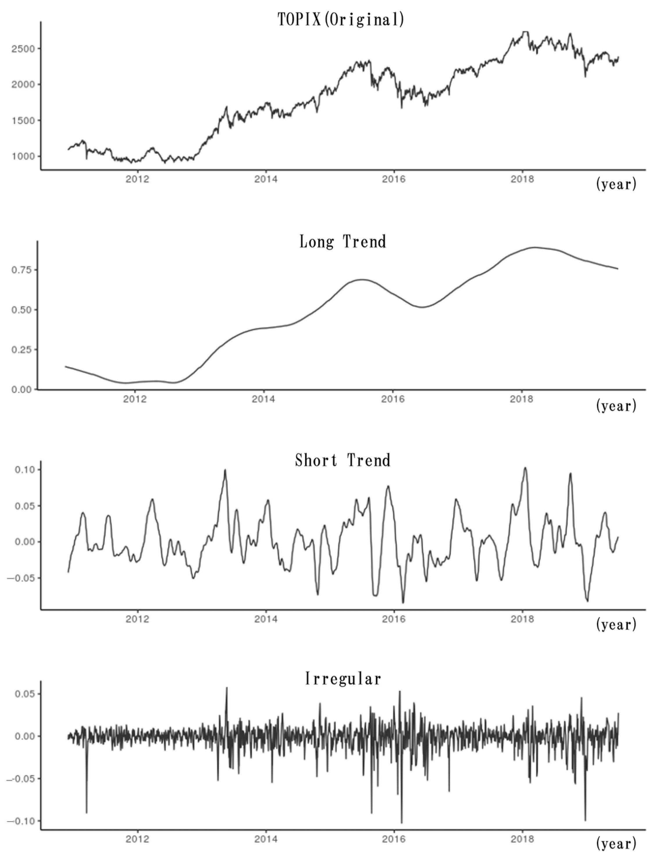
3.1.2. Implications of the Analysis of Average Excess Returns

Although we will discuss specific news events in detail in Section 3.2, it is worth mentioning the overall implications of the results in Table 2 and Table 3. The first implication is that these results (Table 2 and Table 3) confirm a natural phenomenon: Positive news content tends to yield positive reactions, while negative news content leads to negative reactions. The second point is that there is a difference in the magnitude of the earliest response to news delivered intraday and after market close. The intraday (labeled INT) average excess return for 30 events delivered intraday in Table 2 is +0.2%, while the overnight (labeled ON) average excess return for 30 events delivered after market close shown in Table 3 is 0.0%. As this result shows, the market’s initial reaction to intraday news is more significant compared to the reaction to news delivered after market close. In other words, the results suggest that rational market participants react quickly and try to promptly reflect the information into the stock prices for news delivered during trading hours when high liquidity is available for their trading. Furthermore, the existence of performance disparities across different events suggests the potential for developing simple investment strategies tailored to specific events.

Table 4 and Table 5 describe the performance by score; while the impact of news delivered intraday lasts relatively longer for extremely positive (Q10) news or extremely negative (Q1) news, as shown in Table 4, it can be seen that the majority of the impact of the news after market close, as shown in Table 5, tends to be reflected in the next day’s opening price (labeled ON). This result suggests that even if the news is particularly positive or negative in terms of the sentiment, it may take some time for investors and market participants to analyze the future impact of the news on stock prices and implement actual trade executions. In other words, while intraday news is gradually reflected in stock prices over a period of several days, news distributed after market trading hours provides more time to analyze its impact on future stock prices and can be reflected immediately in the next day’s opening price.

The effect of information uncertainty on the relationship between news and stock price drifts, as indicated by Zhang (2006), can be related to the news categories shown in Table 2 and Table 3. While Zhang (2006) defined good or bad news in his main analysis by analyst forecast revisions, the most relevant news categories in our study are “Profit Forecast Increase“ and “Profit Forecast Decrease“. In addition, news categories in our news data that may have a qualitatively similar impact to analyst forecast revisions could include “Exceeding QUICK Consensus Estimate“, meaning positive surprise, and “Missing QUICK Consensus Estimate“, ” Profit Increase”, and ” Profit Decrease”.

In fact, Zhang (2006) suggested that the greater the information uncertainty, the higher the returns following good news and the lower the returns following bad news. In the news data used in our study, news distributed after market trading hours could be relatively more uncertain than news distributed during trading hours. This is because, for news distributed during trading hours, it is possible to use this new information as soon as it is ready to trade the stock at a price at least close to the price quoted at that time, whereas for news distributed after the close of trading, the earliest one can trade the stock is at the opening of the next business day. As we can see from our analysis, the excess return of the “Profit Forecast Increase”, as shown in Table 2, No. 21, is +0.5% for the longest measurement period (for D5), while for the same category in Table 3, No. 16, it is +1.6% (for D4.5). Furthermore, for the “Profit Forecast Decline” (Table 2), No. 26 is equal −1.1%, while in Table 3, No. 18 has a value of −2.5%, which clearly indicates that news distributed after the close of market trading has a greater impact on stock prices. This result is consistent with that of Zhang (2006) and confirms a similar trend regarding the impact of information uncertainty on stock price drifts in the Japanese stock market.

3.1.3. Effects of Each Company’s Market Capitalization

In addition, we believe that we should examine the possibility of identifying different effects on the performance resulting from each company’s market capitalization. Therefore, we conducted an analysis to validate the size effect on the relationship between stock performance and category-based news; the results of the analysis can be found in Appendix A. To examine how the impact of delivered news on stock prices affects small- and large-cap stocks, we compared the performance of the bottom 30% of the stocks and the top 30% of the stocks based on their market capitalization as of 31 March 2022. This analysis reveals differences in the magnitude and timing of stock price behavior following the news due to differences between small- and large-cap stocks.

The results shown in

Table A1. Comparison of stock performance by event for news delivered during trading hours. This presents the average scores and excess returns relative to the TOPIX for each event for intraday news by small- and large-cap stocks, considering different time horizons. For No. 14 and No. 24, which refer to QUICK Consensus, there are no data for the bottom 30% of stocks by market capitalization; so, the data for those small-cap stocks are not included in the analysis here.

No.	News Tag	Average Score		INT (%)		ON (%)		D1 (%)		D3 (%)		D5 (%)
		Small	Large	Small	Large	Small	Large	Small	Large	Small	Large	Small	Large
1	Market Rise	87.1	83.7	2.3	0.7	3.4	0.7	2.4	0.6	2.1	0.6	1.5	0.6
2	Market Decline	14.0	17.8	−2.4	−0.6	−2.0	−0.7	−2.9	−0.8	−4.7	−0.8	−5.6	−0.8
3	Increase in Large-Volume Holdings	49.7	49.6	0.2	0.0	−0.1	0.1	−0.1	0.1	−0.2	0.2	−0.4	0.2
4	Decrease in Large-Volume Holdings	39.4	39.3	−0.2	0.0	0.1	0.0	0.0	0.0	−0.1	0.1	−0.1	0.1
5	Sales Increase	56.5	54.6	0.1	0.0	0.1	0.1	0.1	0.1	0.5	0.0	0.5	0.1
6	Profit Increase	59.3	60.3	−1.4	0.2	−0.5	0.2	−0.9	0.3	−1.1	0.0	−1.8	0.1
7	Rise in Stock Rating	76.6	83.2	1.0	0.2	1.2	0.3	0.7	0.4	1.2	0.6	1.9	0.7
8	Profit increase: Market Rise	93.1	92.2	2.0	0.5	2.4	0.4	1.5	0.4	−1.3	0.5	−1.6	0.5
9	Sales Decrease	40.5	40.9	−0.1	−0.1	0.0	0.0	0.1	0.0	−0.1	0.0	−0.5	0.0
10	Profit Forecast Increase: Market Rise	92.5	93.4	0.9	0.7	2.4	0.7	1.6	0.7	1.5	0.9	0.5	0.9
11	Sales Increase: Market Rise	85.8	94.4	4.9	0.7	7.2	0.6	5.3	0.6	−0.4	0.8	−1.6	0.8
12	Profit Decrease	28.7	36.8	−0.8	−0.1	−0.4	−0.3	0.0	−0.5	0.1	−0.7	−1.0	−0.6
13	Stock Rating Downgrade	13.6	13.9	−0.3	−0.3	0.8	−0.4	0.5	−0.4	−0.3	−0.5	−0.9	−0.4
14	Missing QUICK Consensus Estimate	−	38.2	−	−0.2	−	−0.2	−	−0.3	−	−0.6	−	−0.7
15	Profit Forecast Decrease: Market Decline	7.5	6.0	−0.4	−0.4	−1.5	−0.8	−1.5	−0.9	−2.3	−1.1	−3.3	−1.1
16	Profit Decrease: Market Decline	8.9	7.9	0.2	−0.7	−1.1	−0.3	−1.3	−0.4	−2.4	−0.4	−1.7	−0.5
17	Stock Rating Downgrade: Market Decline	5.0	5.8	1.1	−0.6	0.5	−0.6	−0.8	−0.6	0.7	−0.5	−4.6	−0.4
18	Profit increase: Market Decline	11.5	9.6	−2.1	−0.8	−2.6	−0.5	−4.3	−0.6	−7.1	−0.7	−6.6	−0.7
19	Scandal	50.1	43.2	−2.0	−0.1	−2.2	−0.7	−2.6	−0.7	−3.9	−1.0	−2.7	−0.9
20	Buyback	86.5	82.3	1.1	1.4	3.2	0.7	2.5	0.8	2.0	0.8	1.9	0.9
21	Profit Forecast Increase	76.2	72.6	−0.2	0.2	1.8	0.4	−0.3	0.5	−2.9	0.6	−3.1	0.6
22	Market Rise: Sales Increase	93.3	91.1	1.5	0.9	4.7	0.6	3.2	0.8	1.1	0.9	1.6	0.8
23	Buyback: Market Rise	95.4	93.0	0.0	0.6	0.5	0.2	−0.6	0.1	−0.2	0.3	−1.0	0.4
24	Exceeding QUICK Consensus Estimate	-	72.9	-	0.6	-	0.7	-	0.9	-	0.9	-	1.0
25	Stock Split	77.0	72.9	3.1	1.0	3.7	1.5	3.4	1.6	5.4	1.2	6.5	1.4
26	Profit Forecast Decrease	28.1	24.4	1.1	−0.1	−2.1	−0.8	−2.7	−1.1	−3.5	−1.4	−4.4	−1.3
27	Profit Decrease: Market Rise	88.9	89.7	0.8	0.8	8.8	0.7	7.8	0.7	4.9	0.7	1.1	0.6
28	Profit Forecast Decrease: Market Decline	9.1	10.7	−2.3	−0.9	−1.5	−0.5	−1.9	−0.6	−3.0	−1.0	−3.1	−1.1
29	Falsehood and Disguise	41.5	44.0	4.5	0.0	0.5	−0.8	−2.1	−0.7	1.9	−0.6	1.8	−0.2
30	Sales Increase: Sales Decrease	39.5	41.3	0.0	0.0	0.0	−0.1	0.1	0.0	−0.3	−0.4	−0.7	−0.7

and

Table A2. Comparison of stock performance by event for news delivered after market close. This presents the average scores and excess returns relative to the TOPIX for each event for after-market news by small- and large-cap stocks, considering different time horizons. For No. 12 and No. 21, which refer to QUICK Consensus, there are no data for the bottom 30% of stocks by market capitalization; so, the data for those small-cap stocks are not included in the analysis here.

No.	News Tag	Average Score		ON (%)		INT (%)		D1 (%)		D2.5 (%)		D4.5 (%)
		Small	Large	Small	Large	Small	Large	Small	Large	Small	Large	Small	Large
1	Rise in Stock Rating	78.1	80.5	−0.2	−0.1	0.3	0.1	3.1	1.2	3.6	1.4	2.7	1.5
2	Increase in Large-Volume Holdings	49.9	49.9	0.2	−0.1	−0.1	0.1	0.4	0.3	0.3	0.4	−0.1	0.7
3	Decrease in Large-Volume Holdings	39.2	39.0	0.3	−0.1	−0.2	0.0	−0.3	0.0	−0.7	0.0	−1.0	0.0
4	Stock Rating Downgrade	17.5	20.8	−0.5	0.1	0.3	−0.1	−1.2	−1.0	−3.0	−1.1	−3.2	−1.1
5	Profit Increase	61.0	60.1	0.2	0.0	0.0	0.0	2.1	0.7	1.1	0.5	−1.0	0.5
6	Sales Increase	53.8	53.5	0.0	−0.1	0.0	0.1	0.7	0.2	0.5	0.3	0.1	0.3
7	Profit Decrease	33.2	36.5	0.2	0.1	−0.2	0.0	−1.5	−0.5	−1.8	−0.7	−1.8	−0.7
8	Market Rise	58.5	62.9	−4.8	−0.9	5.1	0.4	9.5	1.0	5.2	0.9	2.8	1.0
9	Sales Decrease	41.0	41.9	0.0	0.0	−0.1	0.0	0.0	−0.2	−0.2	−0.4	−0.6	−0.5
10	Buyback	80.9	78.3	−0.1	−0.1	0.0	0.0	3.9	2.1	2.7	2.0	2.5	2.2
11	Profit Increase: Sales Increase	63.4	64.0	−0.2	−0.1	0.2	0.1	2.8	0.7	1.4	0.6	0.8	0.6
12	Missing QUICK Consensus Estimate	-	37.7	-	0.0	-	0.0	-	−0.6	-	−0.8	-	−0.9
13	Market Decline	40.0	37.3	4.6	1.0	−3.2	−0.3	−6.2	−1.1	−8.6	−1.2	−9.7	−1.2
14	Stock Split	87.6	87.0	−0.2	0.0	0.2	0.1	7.4	4.1	7.5	4.1	7.2	4.2
15	Increased Dividend	81.8	79.2	−0.5	−0.2	0.6	0.2	5.9	2.0	4.6	1.9	4.0	2.1
16	Profit Forecast Increase	71.7	72.7	−0.7	0.0	0.7	0.0	4.2	1.6	1.0	1.5	0.0	1.5
17	No or Reduced Dividend	20.9	22.3	0.3	0.0	−0.2	0.1	−2.1	−1.2	−3.3	−1.7	−3.8	−1.9
18	Profit Forecast Decrease	20.2	25.8	0.2	0.1	0.0	0.0	−2.8	−1.9	−2.9	−2.1	−3.2	−2.1
19	Scandal	40.8	43.9	0.7	0.1	−0.3	−0.1	−1.2	−0.8	−4.5	−1.0	−4.6	−1.2
20	Profit Decrease: Sales Decrease	29.5	32.0	0.2	0.0	−0.2	0.0	−0.4	−0.4	0.0	−0.4	−0.2	−0.4
21	Exceeding QUICK Consensus Estimate	-	73.7	-	−0.1	-	0.1	-	1.9	-	2.1	-	2.2
22	Public Offering	16.6	22.5	0.1	0.1	−0.2	−0.1	−1.8	−3.5	−1.9	−3.9	−4.0	−4.1
23	Profit Increase: Profit Forecast Increase: Sales Increase	80.6	73.8	0.9	−0.1	−1.4	0.1	2.4	1.3	0.5	1.2	−0.2	1.3
24	Profit Decrease: Sales Increase	32.3	31.3	−0.1	0.1	−0.3	0.0	−1.1	−0.9	−1.0	−1.0	−1.4	−1.0
25	Falsehood and Disguise	37.9	44.2	0.3	0.1	0.0	0.1	−1.0	−0.3	0.0	−0.1	−2.0	0.2
26	Change of Listing Market	63.8	63.7	−0.4	0.0	0.2	0.1	5.2	3.5	4.8	3.6	4.5	3.3
27	Enterprise Continuity	50.0	49.9	0.4	−0.2	−0.2	0.2	0.1	0.0	−1.6	1.2	−1.6	1.7
28	Administrative Measures	41.2	46.0	0.1	0.0	−0.4	0.0	−1.0	−0.1	−1.7	0.0	−1.4	0.3
29	Sales Increase: Sales Decrease	39.1	40.1	0.1	0.1	−0.3	−0.1	−0.5	−0.2	−1.4	−0.3	−1.1	−0.3
30	Issue of Share Options	19.6	20.3	−0.1	0.0	0.2	0.3	−1.0	−2.5	−1.7	−2.1	−1.7	−2.4

in Appendix A present the comparison of excess returns relative to the TOPIX for each event for news delivered during trading hours and after market close, respectively. “Small”, in the table, indicates the average scores and performance of small-cap stocks, and “Large” indicates those of large-cap stocks. We found that there has been a large excess return on small-cap stocks, which might be because the volatility of small-cap stocks generally exceeds that of large-cap stocks. Also, the direction of the excess returns of small- and large-cap stocks tends to be the same, especially when it is clear whether the news category is positive or negative. For example, for events that are clearly positive for the stock price, such as “Buyback” and “Stock Split”, both small- and large-cap stocks show relatively large positive excess returns.

Table A3. Comparison of average excess returns for news during trading hours by score. This presents the average excess returns relative to the TOPIX based on a 10th percentile analysis of score levels assigned to intraday news by small- and large-cap stocks.

Quantile	INT (%)		ON (%)		D1 (%)		D3 (%)		D5 (%)
	Small	Large	Small	Large	Small	Large	Small	Large	Small	Large
1	−1.9	−0.7	−1.9	−0.7	−2.4	−0.7	−4.0	−0.8	−4.8	−0.8
2	−0.3	0.0	−0.3	−0.2	−0.6	−0.2	−1.2	−0.3	−1.8	−0.2
3	−0.1	0.0	0.1	0.0	−0.1	0.0	−0.2	0.0	−0.4	0.0
4	−0.2	0.0	0.0	0.0	−0.1	0.0	−0.4	−0.1	−0.6	−0.1
5	0.1	0.0	−0.1	0.0	−0.1	0.0	−0.2	0.0	−0.5	0.0
6	0.2	0.0	−0.1	0.0	−0.1	0.0	−0.2	0.0	−0.3	0.0
7	0.1	0.1	0.3	0.0	0.2	0.1	0.0	0.0	−0.1	0.1
8	0.5	0.1	0.5	0.0	−0.2	0.0	−1.5	0.0	−2.2	0.0
9	1.4	0.4	1.8	0.4	1.1	0.4	0.1	0.4	−0.5	0.4
10	2.6	0.9	3.9	0.7	2.6	0.7	1.1	0.8	−0.2	0.8

and

Table A4. Comparison of average excess returns for news after market close by score. This presents the average excess returns relative to the TOPIX based on a 10th percentile analysis of score levels assigned to after-market news by small- and large-cap stocks.

Quantile	ON (%)		INT (%)		D1 (%)		D2.5 (%)		D4.5 (%)
	Small	Large	Small	Large	Small	Large	Small	Large	Small	Large
1	−0.9	−0.8	−0.5	0.0	−0.5	−0.1	−1.6	−0.1	−1.7	−0.1
2	−0.1	−0.2	−0.1	0.0	−0.1	0.0	−0.5	−0.1	−0.8	−0.1
3	0.3	−0.1	−0.1	0.0	−0.1	0.0	−0.1	−0.1	−0.1	−0.1
4	0.2	0.0	−0.1	0.0	0.1	−0.1	−0.2	−0.1	−0.1	−0.1
5	0.6	0.1	0.0	0.0	0.2	0.0	0.0	−0.1	−0.1	0.0
6	0.8	0.1	0.0	0.0	0.5	0.0	0.1	0.0	0.0	0.0
7	1.5	0.1	−0.1	0.0	0.4	0.0	−0.4	0.0	−0.5	0.0
8	2.6	0.3	−0.2	0.0	0.2	0.0	−0.4	0.0	−0.7	0.0
9	4.0	0.6	−0.3	0.0	0.4	0.0	−0.9	0.0	−1.4	0.0
10	5.6	1.3	−0.4	0.0	0.6	0.1	−0.3	0.1	−0.4	0.2

present the average excess returns relative to the TOPIX based on a 10th percentile analysis of score levels assigned to each news by small- and large-cap stocks. It can be said that the excess returns are larger for small-cap stocks, which are also implied by the results shown in Table A1 and Table A2. Furthermore, as the score level becomes more extreme, as in Quantile 1 and Quantile 10, the period of time after which news distribution tends to have a significant impact on the stock prices in small-cap stocks decreases. On the other hand, for large-cap stocks, the impact of the news tends to be relatively long-lasting.

3.2. Detailed Performance of Each News Category

Below, we focus on four particularly notable news categories identified in our EDA: stock splits, share buybacks, surprises4, and profit increases/decreases. We detail the annual performance and changes in trading volume for each category.

3.2.1. Stock Split

The announcement of stock splits, which can lead to decreased minimum trading lot sizes, generates a stable positive return. Figure 4 depicts performance before and after news related to stock splits, showing consistent outperformance of the TOPIX in the days following the news release. Additionally, Figure 5 shows the performance of stock split news during trading hours, emphasizing its strong outperformance on the same day and the next trading day.

We also examined the effect of sentiment on trading volume. We calculated the volume change ratio as the ratio of the trading volume on the news release day to the average trading volume over the preceding five trading days. The results show that stock split news released after market hours exhibits strong outperformance on the next trading day, while news released during trading hours tends to outperform on the same day and the next trading day. This analysis offers insights into the relationship between sentiment and market dynamics, particularly for news events that exhibit distinct performance patterns.

Figure 6 illustrates the volume change ratio around stock split news released after market hours. The bars in the lightest color represent the immediate post-delivery volume, which remains relatively close to zero compared to the average volume over the preceding five trading days. However, from the next trading day onward, especially within the three trading days following the news release, the volume significantly increases. Figure 7 focuses on stock split news released during trading hours. Unlike the volume change observed after market hours, stock split news delivered during trading hours exhibits substantial volume spikes on the same day. When considering these performance trends, investors tend to react more promptly to stock split news announced during trading hours, while news released after market hours gradually influences stock prices over several trading days.

3.2.2. Buyback

In addition to directly stimulating demand for a company’s own shares, buybacks are also associated with an announcement effect. This effect occurs when corporate management signals to the market that it considers its own stock undervalued. Consequently, buybacks are generally expected to yield positive performance results. As shown in Figure 8, which depicts performance before and after the announcement of share buyback news released after market close, and Figure 9, which illustrates the change in trading volume, it is evident that the TOPIX outperforms with increased volume on the following trading day. Interestingly, the number of share buyback news items decreased significantly in 2020 and 2021, likely reflecting changes in corporate investment behavior during the COVID-19 shock.

3.2.3. Surprise

Next, we examine the effect of earnings surprises based on QUICK Consensus data. Figure 10 illustrates performance before and after positive earnings surprises, while Figure 11 shows the same for negative surprises. Positive surprises generally lead to positive returns; in 2021, the number of positive surprises reached its peak during the pandemic. This suggests that conservative consensus estimates were surpassed during this time. Conversely, negative surprises tend to result in negative performance. However, after the COVID-19 shock, the number of negative surprises decreased slightly in 2020 and 2021, indicating a more conservative consensus in earnings announcements.

Furthermore, we can see the impact of information uncertainty, as indicated by Zhang (2006), regarding the stock price drifts after the news distribution of surprises. It is natural to consider the years 2020 and 2021, immediately after the COVID-19 outbreak, as the situations in which uncertainty increased the most with respect to the valuation of each company during the period of this analysis (from 2013 to 2021). As we mentioned above, after-market news about company valuations tended to be relatively more uncertain than news delivered during market trading hours, with higher returns for good news and lower returns for bad news. The same trend is observed in this analysis, with larger return drifts after the delivery of surprise news in 2020 and 2021, when there was greater information uncertainty. For example, the D4.5 excess return in 2020 in Figure 10 is the highest excess return in our analysis period, and the D4.5 excess return in 2021 in Figure 11 is also clearly the lowest return.

3.2.4. Profit Increase/Decrease

We also investigated the performance around the news related to profit increases (Figure 12) and decreases (Figure 13). While the volume of news related to profit increases declined immediately after the COVID-19 outbreak in 2020, the volume recovered in 2021. However, performance deteriorated to its lowest level during this period. Surprisingly, profit decreases in 2021 slightly outperformed the TOPIX, contrary to the previous trend. These findings suggest a return-reversal tendency after COVID-19.

4. Method

Before proposing an investment strategy using news indicators derived from QUICK terminal data in Section 5, this section explains our methods, which include the creation of news indices and using the index as a trading signal by applying time-series decomposition, and provides an overview of the investment strategy.

4.1. Create a News Index

In this study, news indices are denoted as “NI” and are calculated using Equation (1), which is based on the number of distributed news items linked to listed stocks5. Referencing Tetlock et al. (2008) and Okimoto and Hirasawa (2014), scores of NI are assigned to represent positive and negative sentiments:

$$NI={\displaystyle \frac{P-N}{P+N+1}},$$

(1)

where P represents the number of positive news articles (scores greater than 50) and N represents the number of negative news articles (scores less than 50).

There is a difference between the study by Okimoto and Hirasawa (2014) and our study in terms of the cutoff time for including news in the daily news indices. Okimoto and Hirasawa (2014) used news distributed by 24:00 as the news for the day, whereas we used news distributed by 15:00 as news distributed during stock market trading hours6. Since news distributed during trading hours is more likely to be reflected in stock prices, when analyzing the relationship between news indices and stock indices and proposing investment strategies, it is important to strictly segment the target news by distribution time to more effectively capture the effect of news on stock prices. Figure 14 shows the trend of the created news indices. As per Equation (1), the index level is higher when the number of positive news items is greater than the number of negative news items. The average value of this index over the entire analysis period of this study is −0.088, with a maximum of 0.44 and a minimum of −0.68.

When applying news data to investment strategies, it is important to consider the correlation between the constructed news indices and the TOPIX. Figure 15 shows the results of a simple regression analysis examining the correlation between the news indices and the logarithmic returns of the TOPIX. The estimated intercept and regression coefficient of the regression equation are both significant at the 1% level, estimated at 0.002 and 0.017, respectively, suggesting a positive correlation between the two datasets.

We employed a strategy that assumes a certain correlation between news indices and stock indices, using the divergence between these indices to time investments. During the analysis period (December 2010 to mid-April 2022), the TOPIX, the stock index under analysis, shows a significant annual increase of +10.8%, indicating a clear positive long-term trend. This long-term trend could cause interference, making it difficult to effectively capture short-term divergence between the stock index and the news indices.

To address this, we used time-series decomposition methods proposed and used by Shibata and Miura (1997), Shimadzu and Shibata (2005), and Nakayama and Yokouchi (2018). By extracting and removing the long-term trend from the time-series data under analysis, we aimed to capture the short-term divergence between the news indices and the stock index. The abovementioned studies used a nonparametric trend extraction method called Lowess (locally weighted scatterplot smoothing; Cleveland 1979; Cleveland and Devlin 1982), which itself was proposed by Cleveland (1979) and Cleveland and Devlin (1982), and the study by Shibata and Miura (1997) was the first one to apply it to financial time-series data. In practice, it does not require hypotheses about economic cycles or assumptions of specific time-series models like ARIMA. Therefore, Lowess is said to be a nonparametric smoothing tool in which a user himself determines the appropriate adjustments for its smoothing, like smoothing spans, in an exploratory manner.

We applied this smoothing process to the original time-series data to extract the long-term trend. Additionally, we performed a second smoothing process on the residuals to extract the short-term trend. The residuals after the second smoothing process become the irregular component of a random stationary process. The time-series decomposition of the original time-series data Z(t) using Lowess is represented by Equation (2):

$$Z\left(t\right)=L\left(t\right)+S\left(t\right)+I\left(t\right),$$

(2)

where L(t) represents the long-term trend, S(t) represents the short-term trend, and I(t) represents the irregular component.

Figure 16 shows an example of the time-series decomposition for the TOPIX (including dividends). The original TOPIX time series is decomposed into a long-term trend capturing significant movements and a short-term trend capturing finer fluctuations. We used these two trend-extracted time-series data, standardized individually, to apply Lowess-based time-series decomposition. This can be performed with the sample script of the R function “decomp”, which is given in Appendix B.

4.2. Overview of the Investment Strategy

The investment strategy using news indices employed in this empirical analysis aims to generate positive returns by investing in TOPIX futures (nearest contract month) when the absolute value of the divergence between the short-term trends of the news index and the TOPIX, extracted using the above method, exceeds a set threshold. Specifically, if the short-term trend of the news index significantly exceeds that of the TOPIX on the previous trading day, TOPIX futures are bought at the opening of the next trading day. Conversely, if the short-term trend of the news index significantly falls below that of the TOPIX, TOPIX futures are sold at the opening of the next trading day and the position is closed at the settlement price 10 trading days later. Based on the assumed correlation between the news index and the TOPIX, this strategy captures the temporary divergence between the two time-series data after removing the long-term trend and utilizes the convergence of this divergence. Regarding the use of time-series data, following Nakayama and Yokouchi (2018), we used data from the last three years (750 trading days) for time-series decomposition. Regarding the span of the time-series decomposition in our investment strategy, we used 250 business days for the long-term trend and 10 business days for the short-term trend7. Since the position is held for 10 days once investment in futures begins, the trigger for starting investment is the first day within the last 10 trading days without an existing futures investment when the absolute value of the divergence exceeds the threshold.

The news indices used in this investment strategy are created from news distributed by the end of the trading day, and news distributed after trading hours is used to calculate the news index for the next trading day. There is sufficient time between identifying the divergence in short-term trends and investment in futures at the opening of the next trading day, making this a highly feasible investment strategy in terms of both data acquisition and investment timing.

4.3. Trading Cost Incorporated in Performance

It is important to consider appropriate trading costs in performance measurement in terms of practical applicability of investment strategies in actual trading. This is because, as Chen and Velikov’s (2022) research and other studies pointed out, expected returns on different investment strategies tend to vanish once effective trading costs are taken into account. In our study, we measure a strategy’s performance net of ask–bid spread costs, which are the major trading costs assumed in futures trading. For the ask–bid spread, we used the typical spread cost of TOPIX futures, which are listed on the Osaka Securities Exchange. Specifically, we deducted 2.75 bps from the return of each trade as the ask–bid spread cost, calculated based on the TOPIX futures’ tick size at the end of March 2022.

5. Result

5.1. Simulation Results Using All Categories

This section presents the results of the investment strategy simulation.

Table 6. Simulation results using all categories. The number of trades, number of buys or sells, average return of trades, standard deviation of returns, and win ratio are shown for different thresholds.

Threshold	Number of Trades	Buy/Sell	Average Return	SD	Win Ratio
5%	98	36/62	0.01%	3.63%	50.00%
10%	102	44/58	−0.01%	3.58%	47.06%
15%	81	39/42	0.48%	3.75%	54.32%
20%	49	25/24	0.49%	4.70%	55.10%

shows the number of investments, the breakdown of long and short positions in futures, the average period return8, the unbiased standard deviation, and the win ratio for each 5% threshold during our analysis period. Looking at the levels of the average return and win ratio, we can see that the performance of this investment strategy improves when the threshold exceeds 15%9. The performance of the two patterns with thresholds of 15% and 20% shows a win ratio exceeding 54% and an average period return exceeding +0.40%. In terms of the number of investments, setting the threshold at 15% results in 81 investments, corresponding to about 0.8 investments per month. This means the strategy holds positions for about 7.6 days out of the 20 trading days in a month10.

As mentioned above, during this study’s analysis period, the TOPIX itself experienced a significant rise. This suggests that positive returns could have been achieved by holding futures for a certain period, regardless of the timing of the investment. Therefore, given the nature of this investment strategy, which involves the agile trading of futures, a bias toward long positions could raise doubts about the effectiveness of this strategy when using news indicators. To address this concern, Table 6 shows the number of long and short positions taken during the investment period. For instance, with a threshold set to 15%, out of a total of 81 investments, there are 39 long positions when the short-term trend of the news index exceeds the short-term trend of the TOPIX and 42 short positions when the news index falls below the TOPIX. We can see that there is no significant bias between the number of long and short positions in the setting with a threshold of 15%, showing relatively high performance.

Furthermore,

Table 7. Performance comparison of long/short futures. The number of trades, average return of trades, and win ratio are shown separately for Buy and Sell for different thresholds.

Threshold	Buy			Sell
	Number of Trades	Average Return	Win Ratio	Number of Trades	Average Return	Win Ratio
5%	36	0.61%	63.89%	62	−0.33%	41.94%
10%	44	0.02%	52.27%	58	−0.03%	43.10%
15%	39	0.90%	61.54%	42	0.08%	47.62%
20%	25	0.77%	64.00%	24	0.20%	45.83%

provides a detailed comparison of the performance of long and short positions. Focusing on the threshold of 15% or higher, which shows particularly high performance, the average period return is higher for long positions. With a threshold of 15%, the return for long positions is +0.90%, compared to +0.08% for short positions. While the market’s upward trend might have boosted the performance of long positions, short positions also achieved positive returns. Despite the small sample size, the performance at the 15% or higher thresholds in Table 6 and Table 7 indicates a certain effectiveness of the investment strategy using news indicators.

5.2. Simulation Results Excluding Specific Categories

Here, we show that the performance of this investment strategy can be further improved by refining the news indicators based on the characteristics of the news identified in Section 3. Through EDA, we noticed that news scores in many categories can potentially influence market forecasting ability. However, we also found that many of the news items in the dataset merely convey the current market conditions at that time, which we believe to have a low effect on future stock prices and might reduce the predictive power of the news indicators. We therefore excluded all news tagged with the events “Market Rise” and “Market Decline” from the calculation and constructed new indicators using only news that likely has predictive power.

Table 8. Performance results when excluding news about “Market Rise” and “Market Decline”. The number of trades, number of buys or sells, average return of trades, standard deviation of returns, and win ratio are shown for different thresholds.

Threshold	Number of Trades	Buy/Sell	Average Return	SD	Win Ratio
5%	110	42/68	0.08%	3.58%	53.64%
10%	113	51/62	−0.10%	3.51%	46.02%
15%	95	45/50	0.61%	3.19%	53.68%
20%	66	33/33	0.82%	3.70%	59.09%

shows the simulation results using the new indicators. Comparing the two patterns with a threshold of 15% or higher, which showed good performance with the previous news indicators, we see an increase in the number of investments and an improvement in the average period return. This suggests that the new indicators lead to the discovery of better investment opportunities.

5.3. Change in Investment Timing

Although it slightly deviates from our main research objective, we consider improving the timing of investment in futures positions as a measure to enhance performance. This investment strategy calculates the news indicator using news distributed by 15:00, the closing time of the stock market on the day, and constructs futures positions at the opening of the next business day after sufficient time has elapsed. We believe that advancing this position construction timing from the opening of the next business day to the futures settlement price at 15:15 on the same day could make more effective use of the news indicators. In other words, this measure allows for the use of the news as fresher textual information by starting the investment immediately after calculating the news indicator.

Table 9. Performance at the 15% threshold. The number of trades, number of buys or sells, average return of trades, standard deviation of returns, and win ratio are shown for different thresholds.

Strategy	Number of Trades	Buy/Sell	Average Return	SD	Win Ratio
Original	81	39/42	0.48%	3.75%	54.32%
Proposal 1	95	45/50	0.61%	3.19%	53.68%
Proposal 2	81	39/42	0.47%	3.74%	55.56%
Proposals 1 and 2	95	45/50	0.59%	3.20%	55.79%

shows the changes in the simulation results for the strategy with a 15% threshold, comparing the effect of excluding news tagged with “Market Rise” and “Market Decline” (Proposal 1) and advancing the position construction timing to the same day (Proposal 2). In tuning the threshold as a strategy parameter in 5% increments from 5% to 20%, as described in Section 5.1 and Section 5.2, the threshold of 15% was selected as the parameter at which the number of trades was relatively high compared to the threshold of 20% in terms of their sample size, and good performance was confirmed. While Proposal 1 mainly improves the average period return, Proposal 2 contributes to a slight improvement in the win ratio. The results suggest that advancing the investment timing to a point where the information value is higher can lead to more stable performance.

6. Further Discussion

While almost all prior studies used all available data without interpreting the meaning of the news data, we show that news data might be more effectively used to predict the stock market by considering their content and meaning. Our investment strategy (Proposal 1) shows that excluding news data in categories that have little impact on future stock prices improves the performance of investment strategies that invest in the entire stock market. However, as shown in Section 3, although we find that individual news categories have varying effects on stocks, we are unable to propose investment strategies that take advantage of these individual news categories. An analysis of investment strategies that directly exploit each news category could be addressed using portfolio construction that deals with individual stocks rather than investing in futures, as examined in our study.

Our investment strategy focuses on the short-term trend of the news indices—that is, the time series in which the long-term trend is removed from the original news index—and this strategy performs relatively well. Meanwhile, since the performance of similar investment strategies using long-term trends as the trading signal was significantly underperformed by short-term trend investment strategies, we do not present the results with long-term trends here. Our results are consistent with those of Tetlock (2007), who tested the information theory and supported the sentiment theories that the effect of pessimistic news on the stock market does not last long and that the shock is short-lived and temporary. This is because the results of our analysis might have led to the predictive power of news indices for the stock market by making better use of the short-term information contained in the news index before its effectiveness expires.

Furthermore, considering a comparison with the study by Okimoto and Hirasawa (2014), who used substantially identical news data to cover the same Japanese stock market, there is an apparent difference in the methods employed in their study and ours. Specifically, Okimoto and Hirasawa (2014) examined the information theory and suggested that the sentiment of news data as a whole has an intrinsic effect on the Japanese stock market. On the other hand, our results indicate that specific categories of news, rather than the news as a whole, may be more effective signals of investment strategy. Although the results of the two studies are similar in that they suggest that news data have significant information about the Japanese stock market, an important implication of our study is that looking at news content, which has not been examined in detail in prior studies, could improve predictive power.

Moreover, here, we compare our results to those of Uhl and Novacek (2020), which is a rare study in terms of looking at news content and dynamically selecting news data for predicting stock market returns. They confirmed that their original top news sentiment, which was calculated based on the correlation to equity indices, has predictive power in the US stock market. While the study tested the validity of the method of continuing to pick the most correlated topics with correlation coefficients for various time frames, the sentiment index for the 5-day rolling window was chosen as the representative sentiment index as it had the highest R² value in terms of explanatory power for the S&P 500 return in the regression analysis. Considering that the correlation coefficient between their sentiment index and the stock index tended to drop to almost zero five days after the top topics were selected, as they have shown, it can be said that their top news sentiment captured relatively short-term market fluctuations. We believe that this characteristic of capturing short-term market trends is an important similarity between their study and ours. Having said that, the two studies have apparent differences in the method used to create the indicators. Uhl and Novacek (2020) created indicators by extracting short-term hot topics from news as a kind of supervised method, with the returns of stock index as teachers. On the other hand, our study creates indicators by focusing on news categories related to market fluctuations in an unsupervised manner, then extracting short-term trends by time-series decomposition, and regarding these as hot topics. After all, although the supervised and unsupervised approaches are different, we believe that both methods extract short-term hot topics, and the results of the main analysis are consistent in that those short-term indicators have predictive power for stock markets and demonstrate effectiveness as an investment strategy.

7. Conclusions

In this study, we use category information assigned to news distributed via the QUICK terminal to explore the relationship between the news and the stock market by analyzing changes in stock prices and trading volumes after news distribution for each category. For example, regarding the news distribution of stock splits, which tend to consistently outperform the TOPIX after the announcement, we find that announcements made during trading hours result in significant trading volumes on the announcement day, while announcements made outside of trading hours lead to increased trading volumes over several business days following the announcement. This highlights the different investment behaviors of market participants. Additionally, by analyzing data with an awareness of news categories, we identify the existence of news data that could potentially affect future stock prices and trading volumes.

Furthermore, to verify the relationship between the news and the Japanese stock market, we construct news indicators using scores representing the positive or negative sentiment of the news and simulate investment strategies, using them as trading signals. We confirm that there is a significant relationship between the news and stock indices. Moreover, by refining the news indicators to include only the useful news categories identified in this study, we observe an increase in the number of investments and an improvement in the average period return in the simulations, demonstrating that the value of the information in the news varies across different categories and the significance of considering the content and meaning of the news.

There is, nevertheless, still room for improvement in the news indicators and investment strategy settings developed in this study. The news used to calculate our news indicators was first distributed via the QUICK terminal. It is possible, however, that these distributed news items had already been distributed by other news sources. For example, examining Bloomberg news about the Japanese stock market could improve forecasting power by reflecting the impact from foreign investors. Additionally, although it is not within the scope of this study, to improve the performance of the investment strategy itself, it would be necessary to adopt multiple smoothing methods other than Lowess and verify the optimal investment period. These are research tasks to be undertaken in the future.

References

1. Bollen, Johan, Huina Mao, and Xiaojun Zeng. 2011. Twitter mood predicts the stock market. Journal of Computational Science 2: 1–8. [Google Scholar] [CrossRef]
2. Boudoukh, Jacob, Ronen Feldman, Shimon Kogan, and Matthew Richardson. 2012. Which News Moves Stock Prices? A Textual Analysis. NBER Working Paper 18725. Available online: https://www.nber.org/papers/w18725 (accessed on 6 September 2024).
3. Bybee, Leland, Bryan Kelly, and Yinan Su. 2023. Narrative Asset Pricing: Interpretable Systematic Risk Factors from News Text. The Review of Financial Studies 36: 4759–87. [Google Scholar] [CrossRef]
4. Bybee, Leland, Bryan Kelly, Asaf Manela, and Dacheng Xiu. 2021. Business News and Business Cycles. NBER Working Paper 29344. Available online: https://www.nber.org/papers/w29344 (accessed on 6 September 2024).
5. Chen, Andrew Y., and Mihail Velikov. 2022. Zeroing In on the Expected Returns of Anomalies. Journal of Financial and Quantitative Analysis 58: 968–1004. [Google Scholar] [CrossRef]
6. Cleveland, William S. 1979. Robust Locally Weighted Regression and Smoothing Scatterplots. Journal of the American Statistical Association 74: 829–36. [Google Scholar] [CrossRef]
7. Cleveland, William S., and Susan J. Devlin. 1982. Calendar Effects in Monthly Time Series: Modeling and Adjustment. Journal of the American Statistical Association 77: 520–28. [Google Scholar] [CrossRef]
8. Lee, Heeyoung, Mihai Surdeanu, Bill MacCartney, and Dan Jurafsky. 2014. On the Importance of Text Analysis for Stock Price Prediction. Paper presented at the 9th International Conference on Language Resources and Evaluation, LREC 2014, Reykjavik, Iceland, May 26–31; Available online: https://nlp.stanford.edu/pubs/lrec2014-stock.pdf (accessed on 28 September 2024).
9. Li, Xinyi, Yinchuan Li, Hongyang Yang, Liuqing Yang, and Xiao-Yang Liu. 2019. DP-LSTM: Differential Privacy-Inspired LSTM for Stock Prediction Using Financial News. arXiv arXiv:1912.10806. [Google Scholar]
10. Nakayama, Jun, and Daisuke Yokouchi. 2018. Applying Time Series Decomposition to Construct Index-Tracking Portfolio. Asia-Pacific Financial Markets 25: 341–52. [Google Scholar] [CrossRef]
11. Narayan, Paresh Kumar, and Deepa Bannigidadmath. 2017. Does Financial News Predict Stock Returns? New Evidence from Islamic and Non-Islamic Stocks. Pacific-Basin Finance Journal 42: 24–45. [Google Scholar] [CrossRef]
12. Okimoto, Tatsuyoshi, and Eiji Hirasawa. 2014. Stock market predictability using news indexes. Security Analysis Journal 52: 67–75. [Google Scholar]
13. Roll, Richard. 1988.  R2. The Journal of Finance 43: 541–66. [Google Scholar] [CrossRef]
14. Schumaker, Robert P., and Hsinchun Chen. 2009. Textual analysis of stock market prediction using breaking financial news. The AZFinText system. ACM Transactions on Information Systems 27: 1–19. [Google Scholar] [CrossRef]
15. Shen, Shulin, Le Xia, Yulin Shuai, and Da Gao. 2022. Measuring news media sentiment using big data for Chinese stock markets. Pacific-Basin Finance Journal 74: 101810. [Google Scholar] [CrossRef]
16. Shibata, Ritei, and Ryozo Miura. 1997. Decomposition of Japanese Yen Interest Rate Data Through Local Regression. Asia-Pacific Financial Markets 4: 125–46. [Google Scholar] [CrossRef]
17. Shimadzu, Hideyasu, and Ritei Shibata. 2005. Analysis of bird count series by local regression to explore environmental changes. Journal of the Japan Statistical Society 34: 187–207. (In Japanese). [Google Scholar]
18. Tetlock, Paul C. 2007. Giving Content to Investor Sentiment: The Role of Media in the Stock Market. The Journal of Finance 62: 1139–68. [Google Scholar] [CrossRef]
19. Tetlock, Paul C. 2011. All the News That’s Fit to Reprint: Do Investors React to Stale Information? The Review of Financial Studies 24: 1481–512. [Google Scholar] [CrossRef]
20. Tetlock, Paul C., Maytal Saar-Tsechansky, and Sofus Macskassy. 2008. More Than Words: Quantifying Language to Measure Firms’ Fundamentals. The Journal of Finance 63: 1437–67. [Google Scholar] [CrossRef]
21. Tukey, John Wilder. 1977. Exploratory Data Analysis. Reading: Addison-Wesley. [Google Scholar]
22. Uhl, Matthias W., and Milos Novacek. 2020. When it Pays to Ignore: Focusing on Top News and their Sentiment. Journal of Behavioral Finance 22: 461–79. [Google Scholar] [CrossRef]
23. Zhang, X. Frank. 2006. Information Uncertainty and Stock Returns. The Journal of Finance 61: 105–37. [Google Scholar] [CrossRef]
Figure 1. Distribution of news occurrence times for all analyzed news data from the QUICK terminal. The hours between the dotted lines (9:00–15:00) are the trading hours of the Tokyo stock exchange.
Risks 13 00050 g001
Figure 2. Performance measurement period for news delivered during trading hours.
Risks 13 00050 g002
Figure 3. Performance measurement period for news delivered after trading hours.
Risks 13 00050 g003
Figure 4. Performance based on stock split news delivered after trading hours. This shows the performance after news of stock splits was distributed after market close for each year since 2011 and the number of news distributed, shown by diamond marks based on the right axis.
Risks 13 00050 g004
Figure 5. Performance based on stock split news delivered during trading hours. This shows the performance after intraday-delivered news of stock splits for each year since 2011 and the number of news distributed, shown by diamond marks based on the right axis.
Risks 13 00050 g005
Figure 6. Percentage change in volume based on stock split news delivered after trading hours. The bar labeled “T” shows the volume change ratio as the ratio of the trading volume on the release day of after-market stock split news to the average trading volume over the preceding five trading days. The bar labeled “T+1~T+3” shows the ratio for average volume of the three days from T+1 to T+3 and the bar labeled “T+1~T+5” shows the ratio of the five days from T+1 to T+5.
Risks 13 00050 g006
Figure 7. Percentage change in volume based on stock split news delivered during trading hours. The bar labeled “T” shows the volume change ratio as the ratio of the trading volume on the release day of after-market stock split news to the average trading volume over the preceding five trading days. The bar labeled “T+1~T+3” shows the ratio for average volume of the three days from T+1 to T+3 and the bar labeled “T+1~T+5” shows the ratio of the five days from T+1 to T+5.
Risks 13 00050 g007
Figure 8. Performance based on buyback news delivered after trading hours. This shows the performance after news of buyback was distributed after market close for each year since 2011 and the number of news distributed, shown by diamond marks based on the right axis.
Risks 13 00050 g008
Figure 9. Percentage change in volume based on buyback news delivered after trading hours. This shows the volume change ratio as the ratio of the trading volume on the release day of after-market buyback news to the average trading volume over the preceding five trading days.
Risks 13 00050 g009
Figure 10. Performance based on positive surprise news delivered after trading hours. This shows the performance after news of positive surprise was distributed after market close for each year since 2011 and the number of news distributed, shown by diamond marks based on the right axis.
Risks 13 00050 g010
Figure 11. Performance based on negative surprise news delivered after trading hours. This shows the performance after news of negative surprise was distributed after market close for each year since 2011 and the number of news distributed, shown by diamond marks based on the right axis.
Risks 13 00050 g011
Figure 12. Performance based on profit increase news delivered after trading hours. This shows the performance after news of profit increase was distributed after market close for each year since 2011 and the number of news distributed, shown by diamond marks based on the right axis.
Risks 13 00050 g012
Figure 13. Performance based on profit decrease news delivered after trading hours. This shows the performance after news of profit decrease was distributed after market close for each year since 2011 and the number of news distributed, shown by diamond marks based on the right axis.
Risks 13 00050 g013
Figure 14. Change in the news index.
Risks 13 00050 g014
Figure 15. Relationship between the news index and the TOPIX. The vertical axis represents the logarithmic returns of the TOPIX, and the horizontal axis represents the news index.
Risks 13 00050 g015
Figure 16. Time-series decomposition of the TOPIX. From top to bottom, it shows the TOPIX, long-term trend, short-term trend, and irregular term.
Risks 13 00050 g016