From Stochastic Orders to Volatility Surfaces: Revisiting the One-X Property

Abstract

The One-X property, introduced by Zetocha in a 2023 paper, provides a novel stochastic order with direct implications for constructing arbitrage-free implied volatility surfaces. The current work revisits its theoretical foundations and explores its connections with classical stochastic orders, thereby offering a deeper understanding of its mathematical structure and practical significance in calendar-arbitrage-free modeling. We first present an explicit counterexample to a conjecture raised in Zetocha’s previous paper, and then provide a natural and valid enhancement of this conjecture. After discussing the inherent relations between the One-X property and properties such as $T{P}_2$, $R{P}_2$, and unimodality of density ratio (introcuded by Glasserman and Pirjol in their 2024 papers), we further explore some sufficient conditions to achieve the One-X property for random variables of certain mixture types that are frequently seen in applications.

1. Introduction

Ever since the birth of the Black–Scholes theory Black and Scholes (1973) and local volatility Derman and Kani (1994); Dupire (1994), construction of the arbitrage-free implied volatility (IV) surfaces has become a challenging task. Research on related topics has been receiving continued and widespread attention from both academia and industry. One of the major approaches is to directly model the implied density of the underlying distribution Hagan et al. (2002).

An important concept in the direct modeling approach is the convex order (see Definition 1), which is a stochastic order closely related to the nonexistence of calendar arbitrage: the risk-neutral marginal distributions of the underlying asset should be increasing in convex order to avoid the calendar arbitrage Carr et al. (2011). In other words, if one wants to create two distributions representing the marginals of some forward deflated asset at different expiries, they must obey the increasing convex order. Thanks to this key feature, the discussions of convex order and asset equity modeling have become the main topic in series of recent publications; see Galichon et al. (2014); Wiesel and Zhang (2023); Zetocha (2022, 2023); Glasserman and Pirjol (2024a, 2024b), and Engström et al. (2025).

Despite being a desirable property, the convex order lacks intuitive understanding. It is almost impossible to check or implement in real-world applications, since it requires examining uncountably many integral inequalities for all real-valued convex functions. In view of such inconvenience, more intuitive and practical stochastic orders have recently been discussed. In Zetocha (2023), the concept of One-X order is introduced and is shown to be a sufficient condition for the convex order (see Theorem 1); see also Ohlin (1969). A major advantage of the One-X order is its extreme convenience to apply: one only needs to inspect if the two cumulative distribution functions (CDFs) in consideration intersect only once to tell if they are in One-X order. Moreover, in Glasserman and Pirjol (2024a, 2024b), the authors provided a comprehensive discussion on several novel concepts such as $T{P}_2$, $R{R}_2$, and the unimodality of the density ratio, which are closely related to the convex order. The current paper will further explore the One-X property at a theoretical level and provide a mathematically rigorous discussion of its relation to the other stochastic orders mentioned above.

However, while the One-X order is useful in applications, some basic questions about this concept remain unanswered. For instance, as expected in Conjecture 1 of Zetocha (2023), is it true that the One-X order is also a necessary condition of the convex order? The first contribution of the current paper is to provide a concrete counterexample to this conjecture. By appropriately mixing Gamma and Weibull distributions, in Section 3 we manage to produce two convex-ordered distributions whose CDFs have their graphs intersecting more than once.

We then continue to discover some natural conditions under which the implication of the convex order by the One-X order could be partially reversed. In Section 4 we prove that for each pair of real-analytic random variables with equal mean and in convex order, there exist finitely many consecutive One-X inequalities interpolating between them. This is particularly useful since the most widely used log-Gaussian mixture distributions are analytic.

In Section 5 we will further contribute to the literature by deducing the One-X order from properties such as $T{P}_2\&R{R}_2$ and unimodality of density ratio (see Propositions 4 and 5), thus completing the following indicative chain of implications:

$$\begin{array}{c}\hfill R{R}_2\&T{P}_2\stackrel{\mathrm{Prop}.5}{\Rightarrow }\mathrm{Unimodality}\mathrm{of}\mathrm{Density}\mathrm{Ratio}\stackrel{\mathrm{Prop}.4}{\Rightarrow }\mathrm{One}\text{-}\mathrm{X}\mathrm{Order}\stackrel{\mathrm{Thm}.1}{\Rightarrow }\mathrm{Convex}\mathrm{Order}\\ \hfill \stackrel{\mathrm{Thm}.2}{\Rightarrow }\mathrm{Existence}\mathrm{of}\mathrm{Finitely}\mathrm{Many}\mathrm{One}\text{-}\mathrm{X}\mathrm{Ordered}\mathrm{Interpolations}(\mathrm{Real}\text{-}\mathrm{Analytic}\mathrm{Case}).\end{array}$$

The rest of the paper is organized as the following: in Section 2 we recall the background information, and seek the root of the stochastic orders in actuarial science by making an inter-disciplinary concept comparison in Section 2.3; in Section 6 we find some numerical criterion for pairs of some widely used mixture distributions to satisfy the One-X property; and in the concluding section we briefly mention some challenges in judging stochastic orders and some of our related ongoing and future work.

2. Background

In this section, we will first recall the definitions and properties of some well-known stochastic orders between one-dimensional random variables, which will be used intensively in the later sections. Then we will introduce the dangerousness and the One-X property, which enable us to state and understand the meaning of the conjecture in Zetocha (2023).

2.1. Stochastic Orders and Their Properties

In this section, we present rigorous mathematical definitions of the related stochastic orders, as well as some useful properties. We assume that there are two random variables X and Y with CDFs $F_X$ and $F_Y$, respectively.

Definition 1.

X is smaller than Y in the increasing convex order, denoted as $X{\le }_{icx}Y$, if for any real-valued increasing convex function f,

$$\begin{array}{c}\hfill \mathbb{E}\left[f\right(X\left)\right]\le \mathbb{E}\left[f\right(Y\left)\right],\end{array}$$

(1)

provided both expectations exist.

Since any increasing convex function can be obtained as the limit of linear combinations of the functions in the form $\varphi \left(x\right)={(x-z)}^{+}$, $z\in [0,\infty )$, (1) in the above definition can be replaced by

$$\begin{array}{c}\hfill \forall z\ge 0,\mathbb{E}\left[{(X-z)}^{+}\right]\le \mathbb{E}\left[{(Y-z)}^{+}\right].\end{array}$$

(2)

Using integration by parts, it is also easy to show that (2) is equivalent to the following integral inequality of their corresponding CDFs:

$$\begin{array}{c}\hfill \forall z\ge 0,{\int }_z^{\infty }(1-F_X\left(x\right))dx\le {\int }_z^{\infty }(1-F_Y\left(y\right))dy.\end{array}$$

(3)

If we replace increasing convex function by convex function, then X is called smaller than Y in convex order, denoted as $X{\le }_{cx}Y$. When $\mathbb{E}\left[X\right]=\mathbb{E}\left[Y\right]$, one can show that these two orders are equivalent, i.e., $X{\le }_{icx}Y\iff X{\le }_{cx}Y$; see Theorem 4.A.35 of Shaked and Shanthikumar (2007) for more details. Under the assumption that $\mathbb{E}\left[X\right]=\mathbb{E}\left[Y\right]$, we can therefore use these two definitions in an exchangeable manner.

We now review some of the fundamental but important properties regarding convex order in order to provide additional background on this topic. Some of them are useful for our discussions later in the paper. See Theorems 3.A.2, 3.A.5, 3.A.6, and 3.A.12 of Shaked and Shanthikumar (2007) for more details and their proofs.

Lemma 1.

Here we collect some useful properties or characterizations of the convex order.

1. 

Let X, Y be two random variables, then

$$\begin{array}{c}\hfill X{\le }_{cx}Y\iff -X{\le }_{cx}-Y.\end{array}$$

2. 

(Closure under convolutions.) Assume that we have m pairs of random variables $(X_1,Y_1)$, …, $(X_m,Y_m)$ such that $X_i{\le }_{cx}{Y}_i$ for $i=1,\dots ,m$, then

$$\begin{array}{c}\hfill \sum _{i=1}^m{X}_i{\le }_{cx}\sum _{i=1}^m{Y}_i.\end{array}$$

3. 

If X, Y are independent random variables, then

$$\begin{array}{c}\hfill X{\le }_{cx}Y\iff \mathbb{E}\left[\varphi (X,Y)\right]\le \mathbb{E}\left[\varphi (Y,X)\right]\end{array}$$

for any $\varphi :{\mathbb{R}}^2\to \mathbb{R}$ such that $\varphi (x,y)-\varphi (y,x)$ is convex in x for any y.

4. 

Assume that X and Y are two random variables with equal mean whose CDFs are denoted as F, G, then

$$\begin{array}{c}\hfill X{\le }_{cx}Y\iff {\int }_p^1{F}^{-1}\left(u\right)du\le {\int }_p^1{G}^{-1}\left(u\right)du,\forall p\in [0,1].\end{array}$$

5. 

Assume that X and Y are two random variables with equal mean, then

$$\begin{array}{c}\hfill X{\le }_{cx}Y\iff \mathbb{E}\left[\right|X-a\left|\right]\le \mathbb{E}\left[\right|Y-a\left|\right],\forall a\in \mathbb{R}.\end{array}$$

6. 

(Closure under mixture.) Assume that X, Y, and Θ are random variables. If for any θ in the support of Θ, ${X|}_{\Theta =\theta }{\le }_{cx}{Y|}_{\Theta =\theta }$, then $X{\le }_{cx}Y$.

2.2. One-X Order and a Related Conjecture

To recall the One-X order, we start with the more general definition of the dangerousness ordering which has been introduced to the study of the actuarial science by Müller (1996).

Definition 2.

Given non-negative one-dimensional random variables X and Y whose CDFs are $F_X$ and $F_Y$ respectively, X is called less dangerous than Y, denoted by $X{\le }_{D}Y$, if there exists some $c\ge 0$ such that $F_X\le F_Y$ over $[0,c)$, $F_X\ge F_Y$ over $(c,\infty )$, and $\mathbb{E}\left[X\right]\le \mathbb{E}\left[Y\right]$.

When $\mathbb{E}\left[X\right]=\mathbb{E}\left[Y\right]$ is required, this relation is called One-X in Zetocha (2023); in this case, we will write $X{\le }_{One-X}Y$.

As mentioned before, we have the following implication:

Theorem 1

(Theorem 3 of Zetocha (2023)). Given non-negative one-dimensional random variables X and Y such that $\mathbb{E}\left[X\right]=\mathbb{E}\left[Y\right]$, then $X{\le }_{One-X}Y\Rightarrow X{\le }_{cx}Y$.

The inverse of this theorem is conjectured by Zetocha:

Conjecture 1

(Conjecture 1 of Zetocha (2023)). Given non-negative one-dimensional random variables X and Y whose CDFs are $F_X$ and $F_Y$, respectively. Suppose $F_X$ and $F_Y$ are continuous and strictly increasing functions on ${\mathbb{R}}_{+}$, and $\mathbb{E}\left[X\right]=\mathbb{E}\left[Y\right]$, then $X{\le }_{cx}Y\Rightarrow X{\le }_{One-X}Y$.

By providing a counterexample to this conjecture in the next section, we will show that a single One-X inequality is not enough for a pair of random variables satisfying the convex ordering.

2.3. Inter-Disciplinary Concept Comparison

So far, we have considered several orderings, including the convex order, the One-X order, and the dangerousness order. Some of these concepts occur in financial mathematics, and some of them originate in actuarial science. In this subsection, we will try to make a more systematic summary of these concepts and some results, aiming to build a dictionary between some of the important concepts from the two fields.

For the sake of simplicity, we will work under the assumption that all the distributions are non-negative, continuous, and have the same mean. Given two random variables X and Y with continuous, strictly increasing CDFs and equal mean, we briefly summarize the various stochastic orderings in different contexts in

Table 1. Comparison of stochastic order concepts in different fields.

Financial Mathematics Concepts	Actuarial Science Concepts
One-X Order: $X{\le }_{One-X}Y$	Less Dangerous: $X{\le }_{D}Y$ & equal mean
Increasing Convex Order: $X{\le }_{icx}Y$	Stop-loss Order: $X{\le }_{sl}Y$
Convex Order: $X{\le }_{cx}Y$	Transitive closure of ${\le }_D$: $X{\le }_{D^{*}}Y$.

.

Notice that in each of the first two rows, the concepts are mathematically defined in identical manners, and the two concepts in the third row are shown to be equivalent by Corollary 4.4 Müller (1996). Moreover, the lack of transitivity of ${\le }_{One-X}$ or ${\le }_D$ makes them in-equivalent to ${\le }_{cx}$, and their transitive closure ${\le }_{D^{*}}$ is defined as follows: $X{\le }_{D^{*}}Y$ if there is a sequence of random variables ${\left\{X_n\right\}}_{n=1}^{\infty }$ such that $X=X_1$, $X_n{\le }_D{X}_{n+1}$ and that $X_n\to Y$ weakly. Notice that under the assumption $\mathbb{E}\left[X\right]=\mathbb{E}\left[Y\right]$, it consequently holds that $\mathbb{E}\left[X\right]=\mathbb{E}\left[X_n\right]$ for all $n=1,2,3,\dots$.

3. A Counterexample to Conjecture 1

In this section, we begin by reviewing conditions for the existence of (increasing) convex order between two distributions in specific exponential families. We will then construct two random variables with the same finite mean that are in convex order; moreover, they have continuous and strictly increasing CDFs, but their CDFs cross more than once: this violates the corresponding One-X inequality and becomes a counterexample to Conjecture 1.

3.1. (Increasing) Convex Order Between Exponential Family Distributions

We will consider the Gamma and the Weibull distributions. Conditions on the existence of increasing convex order between two given Gamma or Weibull distributions are given following their definitions. We follow Belzunce et al. (2015) for the notations and the main results in this part.

Definition 3.

(Gamma Distribution) A non-negative continuous one-dimensional random variable X follows the Gamma distribution, denoted by $X\sim G(\alpha ,\beta )$, if its probability density function (PDF) is given by the following:

$$\begin{array}{c}\hfill f\left(x\right)={\displaystyle \frac{x^{\alpha -1}{e}^{(-\frac{x}{\beta })}}{{\beta }^{\alpha }\mathsf{\Gamma }\left(\alpha \right)}},x\in (0,\infty ),\end{array}$$

where $\alpha >0$ is called the shape parameter, and $\beta >0$ is called the scale parameter.

If $X\sim G(\alpha ,\beta )$, then $\mathbb{E}\left[X\right]=\alpha \beta$.

Definition 4

(Weibull Distribution). A non-negative continuous one-dimensional random variable X follows the Weibull distribution, denoted by $X\sim W(\alpha ,\beta )$, if its CDF is given by the following:

$$\begin{array}{c}\hfill F\left(x\right)=1-e^{-{\left({\displaystyle \frac{x}{\alpha }}\right)}^{\beta }},x\in (0,\infty ),\end{array}$$

where $\alpha >0$ is called the scale parameter, and $\beta >0$ is called the shape parameter.

If $X\sim W(\alpha ,\beta )$, then $\mathbb{E}\left[X\right]=\alpha \mathsf{\Gamma }(1+{\displaystyle \frac{1}{\beta }})$.

Given two random variables which follow either the Gamma or the Weibull distributions, let’s state some sufficient conditions to guarantee the existence of an increasing convex order relation between them. These sufficient conditions are adopted from Section 2.9.1 of Belzunce et al. (2015) :

Lemma 2.

Given two random variables $X_i\sim G({\alpha }_i,{\beta }_i),i=1,2$, if ${\alpha }_1>{\alpha }_2$ and ${\alpha }_1{\beta }_1\le {\alpha }_2{\beta }_2$, then $X_1{\le }_{icx}{X}_2$. If ${\alpha }_1{\beta }_1={\alpha }_2{\beta }_2$, then $X_1{\le }_{cx}{X}_2$.

Given $X_i\sim W({\alpha }_i,{\beta }_i),i=1,2$, if ${\beta }_1>{\beta }_2$ and ${\alpha }_1\mathsf{\Gamma }(1+1/{\beta }_1)\le {\alpha }_2\mathsf{\Gamma }(1+1/{\beta }_2)$, then $X_1{\le }_{icx}{X}_2$. If ${\alpha }_1\mathsf{\Gamma }(1+1/{\beta }_1)={\alpha }_2\mathsf{\Gamma }(1+1/{\beta }_2)$, then $X_1{\le }_{cx}{X}_2$.

Here we rely on the fact that if two non-negative random variables with the same mean follow increasing convex order, then they are in convex order; see Theorem 4.A.35 of Shaked and Shanthikumar (2007).

3.2. The Counterexample

We consider the following random variables with the same mean:

$X_i$ is defined as the mixture of $Y_{ij},j=1,2,3$ such that

• $X_i$ equals $Y_{i1}$ with probability $={\displaystyle \frac{1}{2}}$;
• $X_i$ equals $Y_{i2}$ with probability $={\displaystyle \frac{1}{5}}$;
• $X_i$ equals $Y_{i3}$ with probability $={\displaystyle \frac{3}{10}}$,

 where the six independent random variables are as follows:

• $Y_{11}\sim G(3,1/3)$, $Y_{12}\sim G(10,3)$, $Y_{13}\sim W(0.5,1)$;
• $Y_{21}\sim G(1/3,3)$, $Y_{22}\sim G(3,10)$, $Y_{23}\sim W(1/12,1/3)$.

From Lemma 2, it is clear that $Y_{11}{\le }_{cx}{Y}_{21}$, $Y_{12}{\le }_{cx}{Y}_{22}$ for the two pairs of Gamma distributions, and each pair shares the same mean. For the pair of Weibull distributions $Y_{13}$ and $Y_{23}$, notice that ${\beta }_{13}=1>1/3={\beta }_{23}$; moreover, since $\mathsf{\Gamma }(1+1/{\beta }_{13})=\mathsf{\Gamma }\left(2\right)=1$ and $\mathsf{\Gamma }(1+1/{\beta }_{23})=\mathsf{\Gamma }\left(4\right)=6$, it follows

$$\begin{array}{c}\hfill {\displaystyle \frac{\mathsf{\Gamma }(1+1/{\beta }_{13})}{\mathsf{\Gamma }(1+1/{\beta }_{23})}}={\displaystyle \frac{1}{6}}={\displaystyle \frac{{\alpha }_{23}}{{\alpha }_{13}}}.\end{array}$$

Therefore, $Y_{13}{\le }_{icx}{Y}_{23}$ from Lemma 2. Since $X_i$ ($i=1,2$) are mixtures of $Y_{ij}$’s, we have $X_1{\le }_{cx}{X}_2$ by the item 6 of Lemma 1.

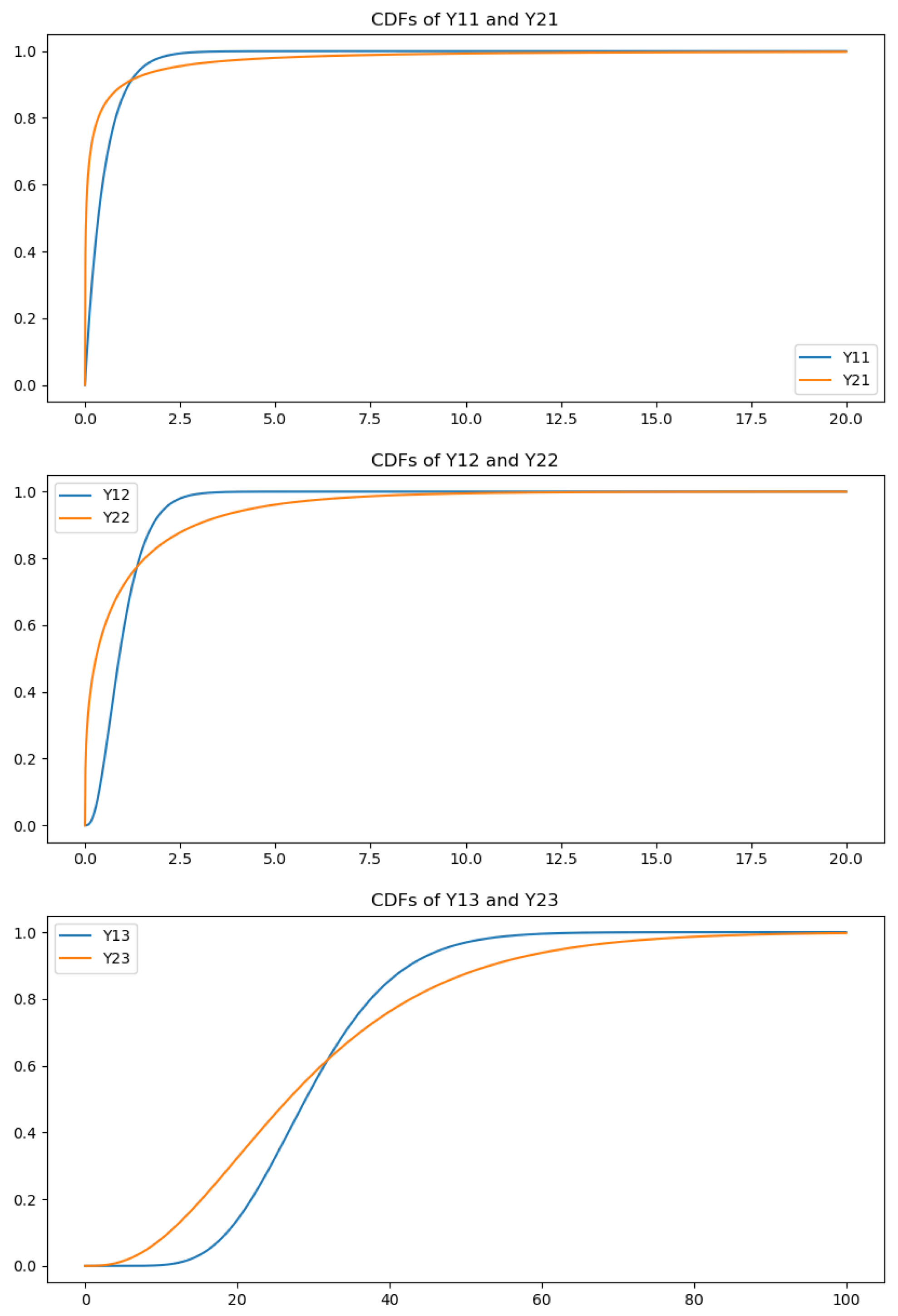
We can also plot the CDFs of each pair of $Y_{1j}$ and $Y_{2j}$ ($j=1,2,3$), and their CDFs satisfy the One-X inequality for each j. According to Theorem 3 of Zetocha (2023), we can therefore conclude that $Y_{1j}{\le }_{cx}{Y}_{2j}$ for each $j=1,2,3$; this is consistent with our analysis above. The plots of each pair of CDFs are shown in Figure 1.

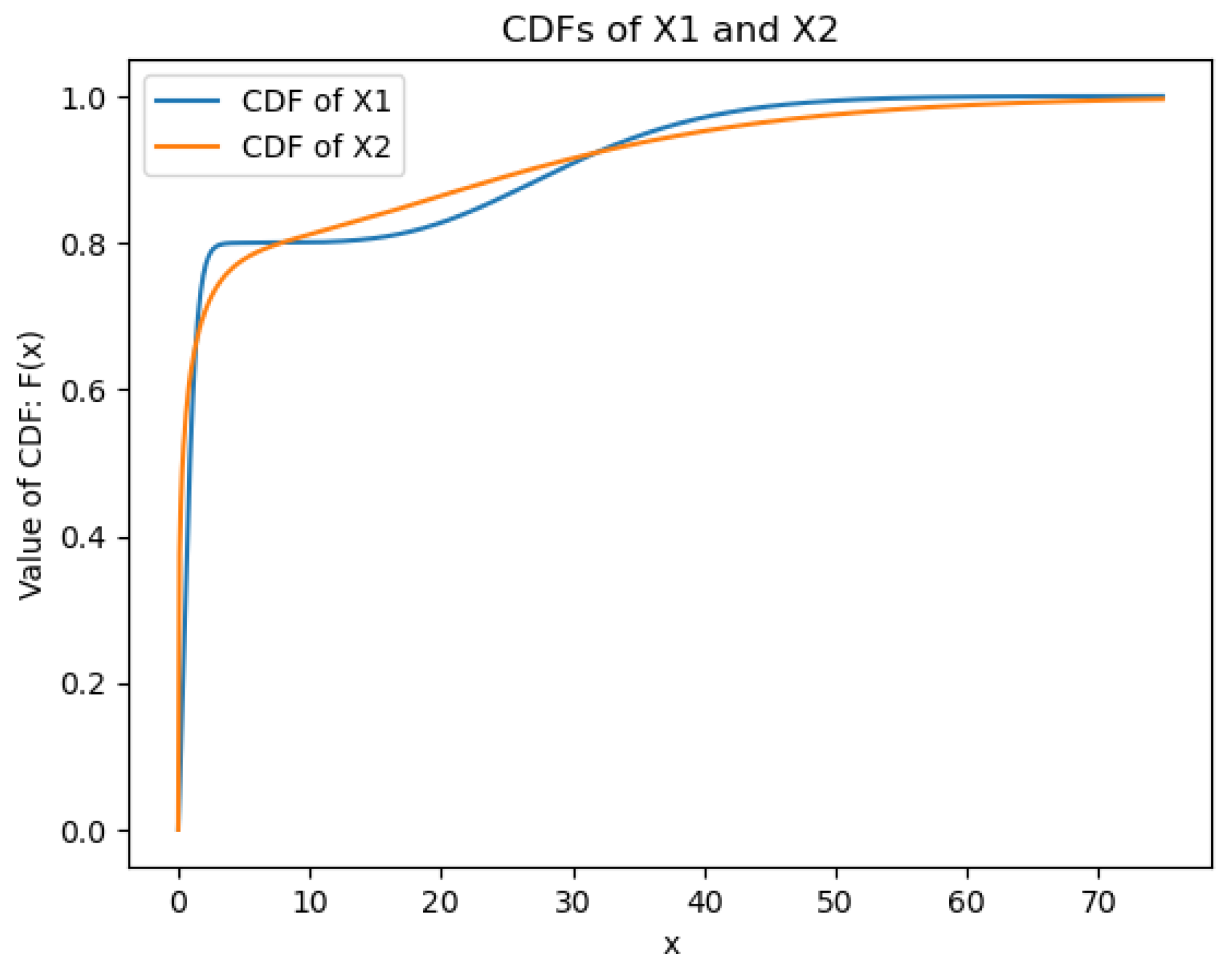
To conclude our argument on this counterexample, let’s show that the CDFs of the two distributions $X_1$ and $X_2$ cross more than once.

Let’s denote the CDF of $X_i$ by $F_i$, $i=1,2$, CDF of $Y_{jl}$ by $G_{jl}$, $j=1,2$; $l=1,2,3$. By our construction, we have

$$\begin{array}{c}\hfill F_i\left(x\right)={\displaystyle \frac{1}{2}}{G}_{i1}\left(x\right)+{\displaystyle \frac{1}{5}}{G}_{i2}\left(x\right)+{\displaystyle \frac{3}{10}}{G}_{i3}\left(x\right),i=1,2,\end{array}$$

defined over $[0,\infty )$.

We consider the difference $H\left(x\right):=F_1\left(x\right)-F_2\left(x\right)$. Notice that the CDFs of $Y_{jl},j=1,2;l=1,2,3$ are continuous; thus, $F_i,i=1,2$ are also continuous, and so is their difference.

If we can find at least two different pairs of values $(x_1,x_2),(x_3,x_4)$ such that $H\left(x_1\right)H\left(x_2\right)<0$ and $H\left(x_3\right)H\left(x_4\right)<0$, then by the Intermediate Value Theorem, we can conclude that there exist $a,b\ge 0$ such that $H\left(a\right)=H\left(b\right)=0$ where $x_1<a<x_2,x_3<b<x_4$, which means $F_1$ and $F_2$ cross at $a,b$, thus, more than once.

For this example, we choose $(x_1,x_2)=(0.5,3)$ and $(x_3,x_4)=(20,40)$. To evaluate the values of $H\left(x\right)$ on these four points, we utilize the well-established Python package SciPy (more details are included in Appendix B):

$$\begin{array}{c}\hfill H\left(0.5\right)=-0.261930,H\left(3\right)=0.054320\Rightarrow H\left(0.5\right)H\left(3\right)<0;\\ \hfill H\left(20\right)=-0.036528,H\left(40\right)=0.018758\Rightarrow H\left(20\right)H\left(40\right)<0.\end{array}$$

Therefore, $X_1{\nleqq }_{One-X}{X}_2$, but we have already shown that $X_1{\le }_{cx}{X}_2$. This completes the counterexample.

We also plot the two CDFs to illustrate their intersections in Figure 2.

4. One-X Interpolation Between Convex Ordered Pairs

Although Conjecture 1 fails in the most general scenario, we may focus on smaller classes of distributions and obtain a partial inverse to the implication “${\le }_{One-X}\Rightarrow {\le }_{cx}$”. Before determining which classes of distributions are viable in practice, let us discuss a general result: a general One-X Interpolation.

As mentioned in Section 2.3, the One-X order (or the dangerousness order) is not transitive, and its transitive closure requires inserting extra terms in between two random variables satisfying the convex order. Theoretically, there might be infinitely many intermediate terms appearing.

However, from a practical point of view, we are mainly interested in the assumptions that two random variables share the same mean, are positive, and have finitely many points of intersection in their CDFs.

The random variables represent the distribution of tradable assets across different expiries, and thus are positive in nature.

Let us consider a few typical underlying assets; we will show that we can always assume they are martingales, and, thus, their marginal distributions share the same mean.

When the underlying is of equity class, the presence of dividends poses challenges for constructing IV and the local volatility surface. One way to bypass this is the pure stock process Buehler (2010): assume that the equity price is $S_t$, the pure stock $X_t$ is defined as $S_t=A_t+B_t{X}_t$ where $A_t+B_t=F_t$ and $F_t$ is the stock’s forward price. As shown in Buehler (2010), $X_t$ is a positive martingale with $\mathbb{E}\left[X_t\right]=1$, and all the pricing theories can be transformed from $S_t$ to $X_t$. In particular, the construction of the IV surface or the implied density will be associated with the $X_t$ process.

When the underlying is of a fixed-income class, the typical options are caps/floors and swaptions. For caps/floors, the underlying is the forward rate which is a martingale under T-forward measure; for swaptions, the underlying is the swap rate which is a martingale under swap measure (for more technical details, see Andersen and Piterbarg (2010)).

Now, let’s consider the assumption that there are only finitely many intersections between the CDFs of two marginal distributions. Notice that the usual density functions in practice are real analytic functions; we can prove the following proposition for two continuous positive probability functions.

Proposition 1.

Given two random variables $X_i$ ($i=1,2$) whose CDFs, denoted by $F_{X_i}$ respectively, are defined on $[0,\infty )$, if their CDFs are real-analytic, then the number of intersections of $F_{X_1}$ and $F_{X_2}$ is at most countable. If we further assume that the density function of $X_2$ dominates that of $X_1$, then there are finitely many intersections.

Proof. 

We begin with covering $[0,\infty )$ by ${\cup }_{n=0}^{\infty }[n,n+1]$. Define $h:=F_{X_2}-F_{X_1}$, h is also analytical, whose zero points correspond to the intersection numbers of $F_{X_1}$ and $F_{X_2}$. Let us show that over each sub-interval $[n,n+1]$, h has finitely many zeros, thus, it has at most countably many zeros. $[n,n+1]$ is a compact set in $R^1$. If h has infinitely many zeros, then by Bolzano–Weierstrass Theorem, the set of zeros has a convergent sub-sequence in $[n,n+1]$. Therefore, by the identity theorem, h must be zero on all of $[n,n+1]$, which implies h is identically zero. This is a contradiction to the assumption that $X_1$ and $X_2$ are different.

Let’s denote the density functions by $f_i$, $i=1,2$. If $X_2$ dominates $X_1$, then ${lim}_{x\to \infty }{\displaystyle \frac{f_2\left(x\right)}{f_1\left(x\right)}}=\infty$. Thus, there exists a positive number A such that $F_{X_1}$ and $F_{X_2}$ intersects at most once over $[A,\infty )$. Following the same argument as above, we can show that $F_{X_1}$ and $F_{X_2}$ only intersect a finite number of times over $[0,A]$. Thus, if $X_2$ dominates $X_1$, their CDFs have only finitely many intersection points.    □

In Proposition 1, we prove the result under the general assumption that the CDF/PDF of the random variables are real-analytic functions, and the proof is from scratch. As discussed below in Section 6.1 and Section 7, we are more interested in the case when the density function is a log Gaussian mixture. In this case, the result of this proposition is a direct consequence of Proposition 4.1 in Glasserman and Pirjol (2023).

From the above discussions, we see that our assumptions are natural yet still cover the cases one can encounter in practice. In the rest of this study, these assumptions will also be our primary assumptions by default. Now, we are ready to state and prove the following theorem, which is one of the main results of this paper:

Theorem 2.

Let X and Y be non-negative one-dimensional random variables with equal finite means, i.e., $\mathbb{E}\left[X\right]=\mathbb{E}\left[Y\right]$. Assume that their cumulative distribution functions $F_X$ and $F_Y$ intersect finitely many times on $[0,\infty )$, and denote the number of intersections by n.

Then the following statements are equivalent:

• Convex order: $X{\le }_{cx}Y$;
• Existence of a finite One-X interpolation: there exist n random variables $Z_1,Z_2,\dots ,Z_n$ such that $Z_1=X$, $Z_n=Y$, and for every $i=1,2,...,n-1$, $Z_i{\le }_{One-X}{Z}_{i+1}$.

That is, the convex order between X and Y can be realized as a finite chain of consecutive One-X orders.

Proof. 

“If” part: Assume the existence of random variables $X=Z_1,Z_2,\dots ,Z_n=Y$ such that

$$\begin{array}{c}\hfill Z_i{\le }_{One-X}{Z}_{i+1}\mathrm{for}i=1,2,\dots ,n-1.\end{array}$$

By definition of the One-X order (Definition 2 and below), each relation

$$Z_i{\le }_{One-X}{Z}_{i+1}$$

implies that $\left(1\right)$ the means coincide, i.e., $\mathbb{E}\left[Z_i\right]=\mathbb{E}\left[Z_{i+1}\right]$, and that $\left(2\right)$ the “stop-loss” order holds. In particular, all the random variables have the same mean.

By Theorem 3 of Zetocha (2023), $Z_i{\le }_{One-X}{Z}_{i+1}\Rightarrow Z_i{\le }_{cx}{Z}_{i+1}$. Since the convex order is transitive, we have

$$X=Z_1{\le }_{cx}{Z}_2{\le }_{cx}...{\le }_{cx}{Z}_n=Y.$$

In particular, we conclude that $X{\le }_{cx}Y$.

“Only-if” part: Assume now that

$$X{\le }_{cx}Y$$

and their CDFs $F_X$, $F_Y$ intersect n times.

Since X, Y have the same mean, $X{\le }_{cx}Y\Rightarrow X{\le }_{icx}Y$. Then, by the classic result of Theorem 1.1 in Chapter IV of Hürlimann (2008), there exists a sequence of random variables $Z_1,Z_2,\dots ,Z_n$ such that

$$X=Z_1{\le }_D{Z}_2{\le }_D\dots {\le }_D{Z}_n=Y.$$

Recalling Definition 2, we have $\mathbb{E}\left[Z_1\right]\le \mathbb{E}\left[Z_2\right]\le \dots \le \mathbb{E}\left[Z_n\right]$. Since $\mathbb{E}\left[X\right]=\mathbb{E}\left[Y\right]$, all the random variables $Z_1,\dots ,Z_n$ share the same mean. In this case, ${\le }_D$ is the same as ${\le }_{One-X}$ (see the first row of Table 1) and thus,

$$X=Z_1{\le }_{One-X}{Z}_2{\le }_{One-X}\dots {\le }_{One-X}{Z}_n=Y,$$

proving the “only-if” part.    □

When $F_X$ and $F_Y$ cross possibly infinitely many times, one needs to replace the finite sequence ${\left\{Z_i\right\}}_{i=0}^n$ in Theorem 2 by a possibly infinite sequence which convergences to Y in both distribution and mean (which is called “stop-loss convergence”). A proof of this generalization can be found in Section 4 of Müller (1996); compare also the transitive closure ${\le }_{D^{*}}$ of the dangerousness order mentioned in Section 2.3. An example where there are infinitely many intersections is given below.

Example 1.

An example where there are infinitely many intersections can be found in Glasserman and Pirjol (2023). Assume that X is a log-normal random variable whose density function is as follows:

$$\begin{array}{c}\hfill f_{LN}(x;\mu ,v):={\displaystyle \frac{1}{\sqrt{2\pi }xv}}exp\left(-{\displaystyle \frac{1}{2v^2}}{\left(ln\left({\displaystyle \frac{x}{\mu }}\right)+0.5v^2\right)}^2\right),\end{array}$$

random variable Y, introduced by Heyde, is defined to have a density function

$$\begin{array}{c}\hfill f_H(x;ϵ,{\kappa }_H):=f_{LN}(x;\mu ,v)\left(1+ϵsin\left({\displaystyle \frac{2\pi {\kappa }_H}{v^2}}ln\left({\displaystyle \frac{x}{\mu }}\right)\right)\right),\end{array}$$

then their CDFs of X and Y have infinitely many intersections.

5. TP₂, RR₂, Unimodality of Density Ratio and Convex Ordering

As mentioned in the introduction, it has been an active research area to understand various conditions which guarantee that there is no calendar arbitrage between two given marginal densities. In the recent work Glasserman and Pirjol (2024a, 2024b), concepts such as $T{P}_2$, $R{R}_2$, and the unimodality of density ratio have been introduced to the field. In particular, various sufficient conditions for the existence of convex order between given marginal densities have been discovered based on the information associated with these concepts. In this section, we study how similarly proposed conditions can lead to the more geometrically intuitive One-X property, which is stronger than (and thus implies) the convex ordering.

5.1. A Brief Review of the Concepts

We begin by recalling the definitions and key properties.

Definition 5

(Total Positivity of Order 2 ($T{P}_2$)). Let $K(x,y)$ be a function defined over the product of intervals $I_x\times I_y$. If it holds

$$\begin{array}{c}\hfill \forall x_1,x_2\in I_x,\forall y_1,y_2\in I_y,x_1<x_2\mathit{and}{y}_1<y_2\Rightarrow det\left[\begin{array}{cc}K(x_1,y_1)& K(x_1,y_2)\\ K(x_2,y_1)& K(x_2,y_2)\end{array}\right]\ge 0,\end{array}$$

then $K(x,y)$ is called totally positive of order 2, denoted as $T{P}_2$. $K(x,y)$ is called strictly $T{P}_2$ if the above determinant is strictly positive.

Definition 6

(Reverse Rule of Order 2 $R{R}_2$)). Let $K(x,y)$ be a function defined over the product of intervals $I_x\times I_y$. If it holds

$$\begin{array}{c}\hfill \forall x_1,x_2\in I_x,\forall y_1,y_2\in I_y,x_1<x_2\mathit{and}{y}_1<y_2\Rightarrow det\left[\begin{array}{cc}K(x_1,y_1)& K(x_1,y_2)\\ K(x_2,y_1)& K(x_2,y_2)\end{array}\right]\le 0,\end{array}$$

then $K(x,y)$ is called reverse rule of order 2, denoted as $R{R}_2$. $K(x,y)$ is called strictly $R{R}_2$ if the determinant above is strictly negative.

These two concepts are obviously in some form of duality, as one sees from the following criteria for $T{P}_2$ and $R{R}_2$:

Proposition 2.

Assume that $K(x,y)>0$ for all $(x,y)\in I_x\times I_y$. Then

1. 

$K(x,y)$ is (strictly) $T{P}_2\iff {\displaystyle \frac{K(x_2,y)}{K(x_1,y)}}$ is (strictly) increasing in y, for any fixed $x_1\le x_2$, and

$K(x,y)$ is (strictly) $R{R}_2\iff {\displaystyle \frac{K(x_2,y)}{K(x_1,y)}}$ is (strictly) decreasing in y, for any fixed $x_1\le x_2$;

2. 

if $K(x,y)$ is differentiable in x, then

$K(x,y)$ is (strictly) $T{P}_2\iff {\displaystyle \frac{\partial }{\partial x}}lnK(x,y)$ is (strictly) increasing in y, and

$K(x,y)$ is (strictly) $R{R}_2\iff {\displaystyle \frac{\partial }{\partial x}}lnK(x,y)$ is (strictly) decreasing in y;

3. 

if $K(x,y)$ is, moreover, twice differentiable, then

$K(x,y)$ is $T{P}_2\iff {\displaystyle \frac{{\partial }^2}{\partial x\partial y}}lnK(x,y)\ge 0$, and

$K(x,y)$ is $R{R}_2\iff {\displaystyle \frac{{\partial }^2}{\partial x\partial y}}lnK(x,y)\le 0$; moreover, the strict cases correspond to strict convexity or concavity.

These properties are well-known and can be easily verified by elementary calculations; see also Section 2.1 of Glasserman and Pirjol (2024b).

Definition 7

(Unimodality of Density Ratio). Assume that there are two non-negative random variables $X_1$ and $X_2$ with the same mean, and that their PDFs $f_i\left(x\right)$ ($i=1,2$) are continuous and positive on the interval $(x_{*},x^{*})$, where we denote $x_{*}=inf\left\{x\in \mathbb{R}:{max}_{i=1,2}\mathbb{P}(X_i\le x)>0\right\}$ and $x^{*}=sup\left\{x\in \mathbb{R}:{max}_{i=1,2}\mathbb{P}(X_i>x)>0\right\}$. We call $X_1$ and $X_2$ satisfy the unimodality of density ratio if there exists $\overline{x}\in (x_{*},x^{*})$ such that the ratio ${\displaystyle \frac{f_1\left(x\right)}{f_2\left(x\right)}}$ is strictly increasing in x over $(x_{*},\overline{x})$, and strictly decreasing over $(\overline{x},x^{*})$.

In real-world applications, $X_1$ and $X_2$ are the marginals of the underlying $S_t$ with $X_1=S_{t_1}$ and $X_2=S_{t_2}$, where $t_1<t_2$ denote the time-to-maturity. In consideration of option pricing, the following result in Glasserman and Pirjol (2024b) is useful:

Proposition 3

(Corollary 3.1 of Glasserman and Pirjol (2024b)). Given a non-negative underlying process $S_t$, and assume that the marginals $S_{t_1}$ and $S_{t_2}$ ($t_1<t_2$ denoting the time-to-maturity) have the same mean. If the density functions of $S_{t_1}$ and $S_{t_2}$ satisfy the unimodality of the density ratio, then

• $C(K,t_2)/C(K,t_1)$ is increasing for $K\in (x_{*},x^{*})$, and
• $P(K,t_2)/P(K,t_1)$ is decreasing for $K\in (x_{*},x^{*})$,

where $C(K,t_i)$ (resp. $P(K,t_i)$) denotes the call (resp. put) option price with strike $=K$ and riskless rate $=0$.

A thorough study of this property is in Section 3 of Glasserman and Pirjol (2024b).

5.2. Relation with the One-X Property

Here we emphasize that instead of directly proving the existence of convex ordering out of the above reviewed conditions, we notice that they actually imply the stronger ordering, the One-X property between marginal CDFs. Firstly, considering the unimodality of the density ratio, we have the following results.

Definition 8

(Number of Sign Changes). For any real-valued function F defined over an interval of $\mathbb{R}$, the number of sign changes of F is defined as follows:

Given an interval I contained in the domain of F,

$$\begin{array}{c}\hfill S^{-}\left(F\right)=\underset{m\in \mathbb{N}}{sup}\underset{x_1,\dots ,x_m\in I}{sup}\left\{S^{-}(F\left(x_1\right),F\left(x_2\right),...,F\left(x_m\right))\right\},\end{array}$$

where for any sequence $a_1,a_2,\dots ,a_m$ of real numbers, $S^{-}(a_1,a_2,\dots ,a_m)$ denotes the number of sign changes among $a_1,\dots ,a_m$ (counted starting from $a_1$ and omitting 0’s).

Remark 1.

Obviously, we have $S^{-}(a_1,\dots ,a_m)\le m-1$.

Proposition 4.

Assume that $S_{t_1}$ and $S_{t_2}$ satisfy the unimodality of density ratio, then $S_{t_1}$ and $S_{t_2}$ satisfy the One-X property, and thus, $S_{t_1}{\le }_{icx}{S}_{t_2}$.

Proof. 

From the definition we have $\mathbb{E}\left[S_{t_1}\right]=\mathbb{E}\left[S_{t_2}\right]$, and there exists $\overline{x}\in (x_{*},x^{*})$ such that the ratio ${\displaystyle \frac{f(x,t_1)}{f(x,t_2)}}$ is increasing in x over $(x_{*},\overline{x})$ and decreasing over $(\overline{x},x^{*})$, where $f(x,t_i)$ denotes the PDFs of $S_{t_i}$ respectively for $i=1,2$.

Rename $f(x,t_i)=f_i\left(x\right)$ with $i=1,2$, and set $h\left(x\right)={\displaystyle \frac{f_1\left(x\right)}{f_2\left(x\right)}}$. Then

$$\begin{array}{c}\hfill h^{\prime }\left(x\right)={\displaystyle \frac{f_1^{\prime }\left(x\right)f_2\left(x\right)-f_1\left(x\right)f_2^{\prime }\left(x\right)}{f_2{\left(x\right)}^2}}.\end{array}$$

Since $h\left(x\right)$ increases on $(x_{*},\overline{x})$, decreases on $(\overline{x},x^{*})$ and $f_2{\left(x\right)}^2>0$, we have

$$\begin{array}{c}\hfill \left\{\begin{array}{c}{f}_1^{\prime }\left(x\right)f_2\left(x\right)-f_1\left(x\right)f_2^{\prime }\left(x\right)\ge 0,x\in (x_{*},\overline{x});\hfill \\ f_1^{\prime }\left(x\right)f_2\left(x\right)-f_1\left(x\right)f_2^{\prime }\left(x\right)\le 0,x\in (\overline{x},x^{*}).\hfill \end{array}\right.\end{array}$$

Since $f_1\left(x\right)f_2\left(x\right)>0$ for $x\in (x_{*},x^{*})$, we have

$$\begin{array}{c}\hfill {\displaystyle \frac{d}{dx}}ln{f}_1\left(x\right)-{\displaystyle \frac{d}{dx}}ln{f}_2\left(x\right)={\displaystyle \frac{f_1^{\prime }\left(x\right)f_2\left(x\right)-f_1\left(x\right)f_2^{\prime }\left(x\right)}{f_1\left(x\right)f_2\left(x\right)}},\end{array}$$

and denoting ${\rho }_i\left(x\right)={\displaystyle \frac{d}{dx}}ln{f}_i\left(x\right)$ ($i=1,2$), we have the following:

$$\begin{array}{c}\hfill \left\{\begin{array}{c}{\rho }_2\left(x\right)-{\rho }_1\left(x\right)<0,x\in (x_{*},\overline{x});\hfill \\ {\rho }_2\left(x\right)-{\rho }_1\left(x\right)>0,x\in (\overline{x},x^{*}).\hfill \end{array}\right.\end{array}$$

In the notation of Belzunce et al. (2015), this exactly means that $S^{-}({\rho }_2-{\rho }_1)=1\mathrm{with}\mathrm{sign}-,+$. By Theorem 2.3.8 of Belzunce et al. (2015), we thus have $S^{-}(f_2-f_1)\le 2$ with sign $+,-,+$ when equality holds.

Since $\mathbb{E}\left[S_{t_1}\right]=\mathbb{E}\left[S_{t_2}\right]$, if $S^{-}(f_2-f_1)=2$ then it holds $S_{t_1}{\le }_{cx}{S}_{t_2}$ according to Theorem 3.A.44 of Shaked and Shanthikumar (2007). Moreover, since $S_t$ is mainly considered as some underlying asset, we may assume $S_t\ge 0$ in practice. Consequently, $S_{t_1}\le S_{t_2}$ implies that $S_{t_1}{\le }_{icx}{S}_{t_2}$.

We therefore only need to show that the number of intersections $S^{-}(f_2-f_1)\ne 0,1$:

• If $S^{-}(f_2-f_1)=0$, there is no intersection between the graphs of $f_1$ and of $f_2$. Without loss of generality, assuming $f_1<f_2$ on $(x_{*},x^{*})$, we would arrive at the following contradiction:

  $$\begin{array}{c}\hfill 0=\mathbb{E}[S_{t_2}-S_{t_1}]={\int }_{x_{*}}^{x^{*}}x\left(f_2\left(x\right)-f_1\left(x\right)\right)dx>0,\end{array}$$

  since $x_{*}\ge 0$.
• If $S^{-}(f_2-f_1)=1$, then the graphs of $f_1$ and $f_2$ intersect at a single point $x_0\in (x_{*},x^{*})$, with signs $-,+$ or $+,-$. Without loss of generality, we can assume the sign is $+,-$, otherwise, we can switch $f_1,f_2$; since ${lim}_{x\to x_{*}}{f}_i\left(x\right)={lim}_{x\to x^{*}}{f}_i\left(x\right)=0$ ($i=1,2$), it always holds $[f_1\left(x\right)-f_2\left(x\right)](x-x_0)>0$, and thus

  $$\begin{array}{c}\hfill 0=\mathbb{E}[S_{t_1}-S_{t_2}]={\int }_{x_{*}}^{x*}[f_1\left(x\right)-f_2\left(x\right)](x-x_0)dx>0,\end{array}$$

  which is impossible.

Therefore, it has to be the case that $S^{-}(f_2-f_1)=2$, according to Theorem 3.A.44 and its proof of Shaked and Shanthikumar (2007), the CDFs of $S_{t_1}$ and $S_{t_2}$ only cross once, and thus $S_{t_1}{\le }_{icx}{S}_{t_2}$.    □

Next, we assume that there exists a positive number $\overline{x}\in (x_{*},x^{*})$ such that the positive density function $f(x,T)$ of the underlying asset $S_T$ is strictly $T{P}_2$ over $(\overline{x},x^{*})$ and strictly $R{R}_2$ over $(x_{*},\overline{x})$. In this case, we say that $f(x,T$) is $R{R}_2\&T{P}_2$ over $(x_{*},x^{*})$. The next proposition states that any two marginal random variables $S_{t_1}$ and $S_{t_2}$ with $t_1<t_2$ satisfy the One-X property.

Proposition 5.

Assume that $f(x,T)$ is differentiable in x. If it is $R{R}_2\&T{P}_2$, that is, $f(x,T)$ is strictly $R{R}_2$ over $(x_{*},\overline{x})$ and strictly $T{P}_2$ over $(\overline{x},x^{*})$, then for any two given $t_1<t_2$, $f(x,t_1)$ and $f(x,t_2)$ satisfy the One-X property, and thus $S_{t_1}{\le }_{icx}{S}_{t_2}$.

Proof. 

We show that the above conditions lead to the same assumptions of Proposition 4. Consider Section 2.2 of Glasserman and Pirjol (2024a), replace f and g by $F(x,t_1)$ and $F(x,t_2)$ with $F(x,t_i)$ being the CDF of the marginal random variable $S_{t_i}$ for $i=1,2$ respectively. Since $f(x,T)$ is differentiable in x and is $T{P}_2$ over $(\overline{x},x^{*})$, by Item (2) of Proposition 2, ${\displaystyle \frac{\partial }{\partial x}}lnf(x,T)$ is increasing in T, which implies that ${\displaystyle \frac{\partial }{\partial x}}lnf(x,t_1)<{\displaystyle \frac{\partial }{\partial x}}lnf(x,t_2)$; notice that this is the right-hand side of (18) in Glasserman and Pirjol (2024a), and we can conclude that $F(x,t_1)$ is convex with respect to $F(x,t_2)$. Then by (17) of Glasserman and Pirjol (2024a), we could then conclude that ${\displaystyle \frac{f(x,t_1)}{f(x,t_2)}}$ is decreasing over $(\overline{x},x^{*})$. With a similar argument, we can also show that ${\displaystyle \frac{f(x,t_1)}{f(x,t_2)}}$ is increasing over $\left(x_{*}\overline{x}\right)$. Therefore, ${\displaystyle \frac{f(x,t_1)}{f(x,t_2)}}$ satisfies the unimodality of density ratio assumption in Proposition 4, which applies here.    □

Remark 2.

According to proposition 2.3 and the examples discussed in Section 4 of Glasserman and Pirjol (2024a), we can see that the assumptions in Proposition 5 are fairly natural and may see a wide range for applications.

Remark 3.

From the discussions in Section 2.2 of Glasserman and Pirjol (2024a), we can also see that if the given marginal random variables have strictly increasing CDFs over $(x_{*},x^{*})$, then the conditions in Proposition 4 and in Proposition 5 should be equivalent.

5.3. Examples

Though we already see in Section 4 that One-X property is not a necessary condition for convex order between distributions, it is still a very intuitive, easy to check condition, and can be verified in many practical situations.

The two propositions above provide practical methods to check the “One-X” property directly from their density functions; this will be particularly useful when the density functions are parametrized and differentiable. Below, we present some such examples.

The conditions discussed in Propositions 4 and 5 are not uncommon, especially for some distributions with parametric density functions. In this part, we will look at a few examples that are widely used in financial modeling.

Example 2

(Log-Normal Distribution). Log-normal distribution (whose mean is m) is defined over $[0,\infty )$ with the following density function:

$$f(x,T;m,\sigma )={\displaystyle \frac{1}{\sqrt{2\pi T}x\sigma }}{e}^{-{\displaystyle \frac{{(ln\left(\frac{x}{m}\right)+\frac{1}{2}{\sigma }^{2}T)}^2}{2{\sigma }^{2}T}}},m>0,\sigma >0,x\in [0,\infty ).$$

By replacing v by $\sigma \sqrt{T}$ in Lemma 3.2 of Glasserman and Pirjol (2024a), one can conclude that $f(x,T;m,\sigma )$ is $R{R}_2$ over $(0,m]$ and $T{P}_2$ over $[m,\infty )$, which is the condition of Proposition  5.

Example 3

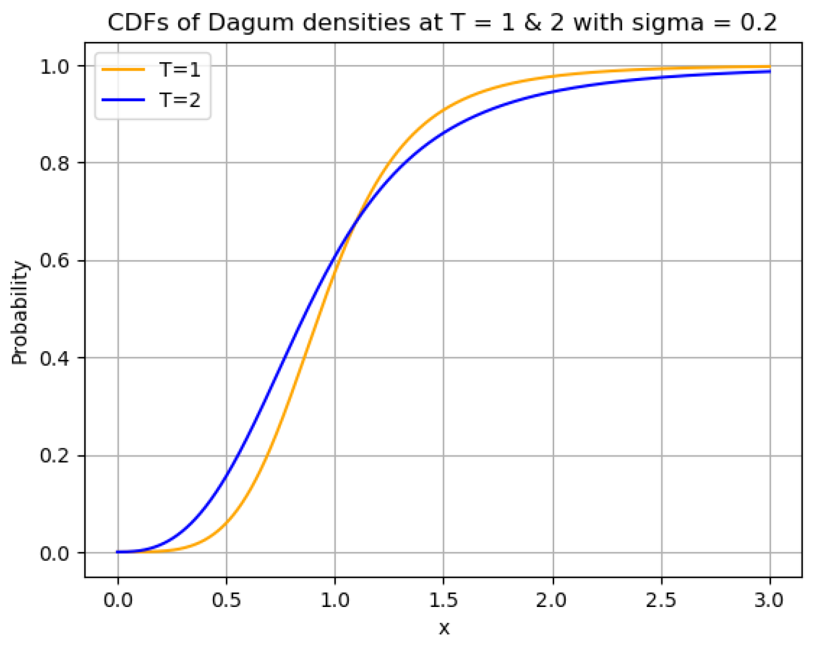
(Dagum Distribution). The density of the Dagum distribution $f_D(x,T)$ over $(0,\infty )$ is given by the following:

$$\begin{array}{c}\hfill f_D(x,T):=(a\left(T\right)-1){\left(1+x^{-a\left(T\right)}\right)}^{{\displaystyle \frac{1}{a\left(T\right)}}-2}{x}^{-a\left(T\right)-1},a\left(T\right)={\displaystyle \frac{1}{\sqrt{1-e^{-{\sigma }^{2}T}}}}.\end{array}$$

By Proposition 4.3 of Glasserman and Pirjol (2024a), the Dagum density has constant mean 1, and it is $T{P}_2$ if $x\ge 1$, $T>0$, and is $R{R}_2$ if $x\le 1$, $T>0$, thus, satisfying the conditions of Proposition  5.

This means that for different values of T, the CDFs of Dagum distributions cross only once. Below is an example:

With $\sigma =0.2$, the CDFs of $f_D(x,1)$ and $f_D(x,2)$ are plotted in Figure 3, which clearly shows a single intersection of the graphs of these CDFs on $(0,3)$.

Example 4

(Scalar Diffusion). Assume that $X_t$ is a one-dimensional continuous martingale diffusion and a non-negative strong Markov process. The density function of the marginal distribution $X_T$ is denoted as $f(x,T)$. Then according to the analysis in Section 4.1 of Glasserman and Pirjol (2024a), $f(x,T)$ is $R{R}_2$ over $(0,X_0]$ and $T{P}_2$ over $[X_0,\infty )$, thus, it satisfies the conditions in Proposition 5.

Example 5

(Continuous Mixture of Log-Normal Distributions). Consider a family of distributions whose density functions are parametrized by T and defined as follows:

$$h(x,T)={\int }_0^{\infty }f(x,T;m,\sigma )w\left(\sigma \right)d\sigma ,$$

where $f(x,T;m,\sigma )$ is the same density function discussed in Example 2, $w\left(\sigma \right)$ satisfies (1) w is a positive function; (2) w is at least first order differentiable; (3) ${\displaystyle \frac{\sigma w^{,}\left(\sigma \right)}{w\left(\sigma \right)}}$ is a decreasing function with respect to σ.

Then by Proposition 4.1 of Glasserman and Pirjol (2024a), $h(x,T)$ satisfies the conditions of Proposition  5.

Example 6

(Heston Model).

Assume that the asset price process is modeled using the Heston model:

$$\begin{array}{cc}\hfill d{S}_t& =\sqrt{v_t}{S}_{t}d{W}_t^1,\hfill \\ \hfill d{v}_t& =(a-\theta v_t)dt+\sigma \sqrt{v_t}d{W}_t^2,\hfill \\ \hfill d{W}_t^{1}d{W}_2^2& =\rho dt.\hfill \end{array}$$

$S_t$ is a martingale; thus, all its marginal distributions have the same mean. Denote the density function of $S_T$ by $f(x,T)$, based on the analysis in Section 3.4.3 of Glasserman and Pirjol (2024b), $f(x,T)$ satisfies the conditions of Proposition 4.

6. One-X Property for Mixture Distributions

The criteria described in Propositions 4 and 5 work well for distributions in the same family with parametrized density functions, as shown in the above examples. However, for more sophisticated density functions, such as mixtures of parametrized families, the conditions for those properties are usually less obvious to verify. In this section, we find conditions that detect the One-X inequality for two widely used families of mixture distributions. In contrast to the analytical criteria obtained before, we highlight that the criteria in Propositions 6 and 7 only contain finitely many numerical conditions and are thus suitable for practical applications.

The main idea is inspired by the proof of Proposition 4: Assume that on some interval $(x_{*},x^{*})$ we are given two positive random variables X, Y with the same mean, and their PDFs are absolutely continuous, denoted as $f_X$ and $f_Y$. We only need to find conditions to make sure that $S^{-}(f_Y-f_X)\le 2$, then, since $\mathbb{E}\left[X\right]=\mathbb{E}\left[Y\right]$, we have $S^{-}(f_Y-f_X)=2$ according to the proof of Proposition 4. If we further assume that ${lim}_{x\to x_{*}}{\displaystyle \frac{f_Y\left(x\right)}{f_X\left(x\right)}}>1$ or ${lim}_{x\to x^{*}}{\displaystyle \frac{f_Y\left(x\right)}{f_X\left(x\right)}}>1$, then the signs of $f_Y-f_X$ must be $+,-,+$, and thus $X{\le }_{One-X}Y$.

The problem of checking the One-X ordering is therefore reduced to finding effective conditions to ensure $S^{-}(f_Y-f_X)\le 2$ even for complicated density functions, such as the mixtures of parametrized density families. To this end, we will rely on the generalized Descartes’ sign rule (see the Appendix of Glasserman and Pirjol (2023), or Theorem 3.1 of Jameson (2006)) that bounds the number of solutions to $f_Y\left(x\right)-f_X\left(x\right)=0$.

Theorem 3

(The generalized Descartes’ sign rule). Given real numbers $a_i,b_i$ ($i=1,\dots ,m$), and assume that the function $G\left(x\right)$ is of the following form:

$$\begin{array}{c}\hfill G\left(x\right)=\sum _{i=1}^m{a}_i{e}^{b_{i}x},b_1>b_2>...>b_m,\end{array}$$

(4)

then $G\left(x\right)$ has at most $S^{-}(a_1,a_2,...,a_m)$ zeros, which is also an upper bound of its sign changes.

We now apply this theorem to study the One-X property for some mixtures of distributions commonly seen in industry applications.

6.1. Mixtures of Log-Normal Distribution with Fixed Variance

These mixtures are direct generalizations of the log-normal distributions used in the Black–Scholes model, and are widely used in financial simulations such as fitting the W-shape volatility smile observed before earnings announcements, for more details, see Glasserman and Pirjol (2023).

Assume that the density functions of X and Y are mixtures of log-normals with the same variance parameter $\sigma$, i.e., for $t>0$ we have PDFs:

$$\begin{array}{c}\hfill f_X\left(t\right)=\sum _{i=1}^m{p}_i{\displaystyle \frac{1}{\sqrt{2\pi }\sigma t}}{e}^{-{\displaystyle \frac{{(lnt-ln{\mu }_i)}^2}{2{\sigma }^2}}}\mathrm{and}{f}_Y\left(t\right)=\sum _{i=1}^n{q}_i{\displaystyle \frac{1}{\sqrt{2\pi }\sigma t}}{e}^{-{\displaystyle \frac{{(lnt-ln{\tau }_i)}^2}{2{\sigma }^2}}},\end{array}$$

(5)

where the weights $p_i,q_j>0$ satisfy ${\sum }_{i=1}^m{p}_i={\sum }_{j=1}^n{q}_j=1$. Then

$$\begin{array}{c}\hfill f_Y\left(t\right)-f_X\left(t\right)={\displaystyle \frac{e^{-\frac{{(lnt)}^2}{2{\sigma }^2}}}{\sqrt{2\pi }\sigma t}}\left(\sum _{j=1}^n{q}_j{e}^{-{\displaystyle \frac{{(ln{\tau }_j)}^2}{2{\sigma }^2}}}{e}^{{\displaystyle \frac{ln{\tau }_j}{{\sigma }^2}}lnt}-\sum _{i=1}^m{p}_i{e}^{-{\displaystyle \frac{{(ln{\mu }_i)}^2}{2{\sigma }^2}}}{e}^{{\displaystyle \frac{ln{\mu }_i}{{\sigma }^2}}lnt}\right),\end{array}$$

and since ${\displaystyle \frac{1}{\sqrt{2\pi }\sigma t}}{e}^{-{\displaystyle \frac{{(lnt)}^2}{2{\sigma }^2}}}>0$, the number of zeros of $f_Y-f_X$ is the same as that of

$$\begin{array}{c}\hfill \sum _{j=1}^n{q}_j{e}^{-{\displaystyle \frac{{(ln{\tau }_j)}^2}{2{\sigma }^2}}}{e}^{{\displaystyle \frac{ln{\tau }_j}{{\sigma }^2}}lnt}-\sum _{i=1}^m{p}_i{e}^{-{\displaystyle \frac{{(ln{\mu }_i)}^2}{2{\sigma }^2}}}{e}^{{\displaystyle \frac{ln{\mu }_i}{{\sigma }^2}}lnt}.\end{array}$$

Now, since $t\mapsto lnt$ is a monotone increasing function for $t>0$, if we set $s=lnt$, the number of zeros of $f_Y\left(t\right)-f_X\left(t\right)$ is the same as the following:

$$\begin{array}{c}\hfill h\left(s\right):=\sum _{j=1}^n{q}_j{e}^{-{\displaystyle \frac{{(ln{\tau }_j)}^2}{2{\sigma }^2}}}{e}^{{\displaystyle \frac{ln{\tau }_j}{{\sigma }^2}}s}-\sum _{i=1}^m{p}_i{e}^{-{\displaystyle \frac{{(ln{\mu }_i)}^2}{2{\sigma }^2}}}{e}^{{\displaystyle \frac{ln{\mu }_i}{{\sigma }^2}}s}.\end{array}$$

(6)

After rearranging and combining the terms of $h\left(s\right)$, we may assume that it is of the form $h\left(s\right)={\sum }_{i=1}^M{a}_i{e}^{b_{i}s}$ with $b_1>b_2>...>b_M$, where $b_i$ is of the form ${\displaystyle \frac{ln{\mu }_k}{{\sigma }^2}}$ or ${\displaystyle \frac{ln{\tau }_l}{{\sigma }^2}}$, and $a_i=p_k{e}^{-{\displaystyle \frac{{(ln{\mu }_k)}^2}{2{\sigma }^2}}}$ or $q_l{e}^{-{\displaystyle \frac{{(ln{\tau }_l)}^2}{2{\sigma }^2}}}$ for some $k\in \{1,\dots ,m\}$ or $l\in \{1,\dots ,n\}$, respectively. If it occurs that ${\mu }_k={\tau }_l$ for some $k\in \{1,\dots ,m\}$ and $l\in \{1,\dots ,n\}$, then the corresponding coefficient $a_i$ is $q_l{e}^{-{\displaystyle \frac{{(ln{\tau }_l)}^2}{2{\sigma }^2}}}-p_k{e}^{-{\displaystyle \frac{{(ln{\mu }_k)}^2}{2{\sigma }^2}}}$.

Thanks to Theorem 3, we now have the following

Proposition 6

(One-X criteria for mixtures of log-normal distributions). Let X and Y be positive random variables whose density functions are given by (5), and let $h\left(s\right)={\sum }_{i=1}^M{a}_i{e}^{b_{i}s}$ be defined as in (6). If $\mathbb{E}\left[X\right]=\mathbb{E}\left[Y\right]$ and $S^{-}(a_1,\dots ,a_M)\le 2$ (in particular, if $M\le 3$), then either $X{\le }_{One-X}Y$ or $Y{\le }_{One-X}X$.

Moreover, assuming that ${\mu }_1>{\mu }_2>...>{\mu }_m$ and ${\tau }_1>{\tau }_2>...>{\tau }_n$, if one of the following conditions is satisfied:

(1) 

${\tau }_n\le {\mu }_m$ and $q_n>p_m$ when ${\tau }_n={\mu }_m$, or

(2) 

${\tau }_1\ge {\mu }_1$ and $q_1>p_1$ when ${\tau }_1={\mu }_1$,

then $X{\le }_{One-X}Y$.

Proof. 

Since $\mathbb{E}\left[X\right]=\mathbb{E}\left[Y\right]$ and $S^{-}(a_1,\dots ,a_M)\le 2$, by the proof of Proposition 4, we have $S^{-}(a_1,\dots ,a_M)=2$. The signs of $f_Y-f_X$ may be either $+,-,+$ or $-,+,-$, and the order $X{\le }_{One-X}Y$ corresponds to $+,-,+$. Therefore, the second part of this proposition will be established once we show that the extra conditions will lead to either ${lim}_{t\to 0}{\displaystyle \frac{f_Y\left(t\right)}{f_X\left(t\right)}}>1$ or ${lim}_{t\to \infty }{\displaystyle \frac{f_Y\left(t\right)}{f_X\left(t\right)}}>1$. Since

$$\begin{array}{c}\hfill {\displaystyle \frac{f_Y\left(t\right)}{f_X\left(t\right)}}={\displaystyle \frac{{\sum }_{j=1}^n{q}_j{e}^{-\frac{{(ln{\tau }_j)}^2}{2{\sigma }^2}}{e}^{\frac{ln{\tau }_j}{{\sigma }^2}lnt}}{{\sum }_{i=1}^m{p}_i{e}^{-\frac{{(ln{\mu }_i)}^2}{2{\sigma }^2}}{e}^{\frac{ln{\mu }_i}{{\sigma }^2}lnt}}}={\displaystyle \frac{{\sum }_{j=1}^n{q}_j{e}^{-\frac{{(ln{\tau }_j)}^2}{2{\sigma }^2}}{t}^{\frac{ln{\tau }_j}{{\sigma }^2}}}{{\sum }_{i=1}^m{p}_i{e}^{-\frac{{(ln{\mu }_i)}^2}{2{\sigma }^2}}{t}^{\frac{ln{\mu }_i}{{\sigma }^2}}}},\end{array}$$

it is then obvious that when Condition (1) is satisfied,

$$\begin{array}{c}\hfill \underset{x\to 0}{lim}{\displaystyle \frac{f_Y\left(t\right)}{f_X\left(t\right)}}=\underset{x\to 0}{lim}{\displaystyle \frac{f_Y\left(t\right)t^{-\frac{ln{\tau }_n}{{\sigma }^2}}}{f_X\left(t\right)t^{-\frac{ln{\tau }_n}{{\sigma }^2}}}}=\underset{x\to 0}{lim}{\displaystyle \frac{{\sum }_{j=1}^{n-1}{q}_j{e}^{-\frac{{(ln{\tau }_j)}^2}{2{\sigma }^2}}{t}^{\frac{(ln{\tau }_j-ln{\tau }_n)}{{\sigma }^2}}+q_n{e}^{-\frac{{(ln{\tau }_n)}^2}{2{\sigma }^2}}}{{\sum }_{i=1}^{m-1}{p}_i{e}^{-\frac{{(ln{\mu }_i)}^2}{2{\sigma }^2}}{t}^{\frac{(ln{\mu }_i-ln{\tau }_n)}{{\sigma }^2}}+p_m{e}^{-\frac{{(ln{\mu }_m)}^2}{2{\sigma }^2}}{t}^{\frac{(ln{\mu }_m-ln{\tau }_n)}{{\sigma }^2}}}},\end{array}$$

thus, ${lim}_{t\to 0}{\displaystyle \frac{f_Y\left(t\right)}{f_X\left(t\right)}}=\infty >1$ when ${\tau }_n<{\mu }_m$, and ${lim}_{t\to 0}{\displaystyle \frac{f_Y\left(t\right)}{f_X\left(t\right)}}={\displaystyle \frac{q_n}{p_m}}>1$ when ${\tau }_n={\mu }_m$.

Similarly, when Condition (2) is satisfied, we have

$$\begin{array}{c}\hfill \underset{x\to \infty }{lim}{\displaystyle \frac{f_Y\left(t\right)}{f_X\left(t\right)}}=\underset{x\to \infty }{lim}{\displaystyle \frac{f_Y\left(t\right)t^{-\frac{ln{\tau }_1}{{\sigma }^2}}}{f_X\left(t\right)t^{-\frac{ln{\tau }_1}{{\sigma }^2}}}}=\underset{x\to \infty }{lim}{\displaystyle \frac{{\sum }_{j=2}^n{q}_j{e}^{-\frac{{(ln{\tau }_j)}^2}{2{\sigma }^2}}{t}^{\frac{(ln{\tau }_j-ln{\tau }_1)}{{\sigma }^2}}+q_1{e}^{-\frac{{(ln{\tau }_1)}^2}{2{\sigma }^2}}}{{\sum }_{i=2}^m{p}_i{e}^{-\frac{{(ln{\mu }_i)}^2}{2{\sigma }^2}}{t}^{\frac{(ln{\mu }_i-ln{\tau }_1)}{{\sigma }^2}}+p_1{e}^{-\frac{{(ln{\mu }_1)}^2}{2{\sigma }^2}}{t}^{\frac{(ln{\mu }_1-ln{\tau }_1)}{{\sigma }^2}}}},\end{array}$$

thus, ${lim}_{t\to \infty }{\displaystyle \frac{f_Y\left(t\right)}{f_X\left(t\right)}}=\infty >1$ when ${\tau }_1>{\mu }_1$, and ${lim}_{t\to \infty }{\displaystyle \frac{f_Y\left(t\right)}{f_X\left(t\right)}}={\displaystyle \frac{q_1}{p_1}}>1$ when ${\tau }_1={\mu }_1$.    □

6.2. Mixtures of Generalized Gamma Distributions

We now discuss the One-X property for mixtures of generalized gamma distributions with fixed shape parameters. These distributions are useful in financial mathematics as many other distributions are their special cases, such as the half-normal distributions, Weibull distributions, and Rayleigh distributions, etc. We begin by recalling the following:

Definition 9

(Generalized Gamma Distribution). A random variable is said to follow a generalized Gamma distribution with shape parameters $p,q>0$ and scale parameter $\alpha >0$, if its density function is defined as follows:

$$\begin{array}{c}\hfill f\left(t\right)={\displaystyle \frac{(p/{\alpha }^q)}{\mathsf{\Gamma }(q/p)}}{t}^{q-1}{e}^{-{(t/\alpha )}^p},\forall t\in (0,\infty ).\end{array}$$

Assume that density functions of X, Y are mixtures of generalized Gamma distributions with the same shape parameters, i.e., with $u_i,v_j>0$ satisfying ${\sum }_{1=1}^m{u}_i={\sum }_{j=1}^n{v}_j=1$, the PDFs are given for $t>0$ as

$$\begin{array}{c}\hfill f_X\left(t\right)=\sum _{i=1}^m{u}_i{\displaystyle \frac{(p/{\alpha }_i^q)}{\mathsf{\Gamma }(q/p)}}{t}^{q-1}{e}^{-{(t/{\alpha }_i)}^p}\mathrm{and}{f}_Y\left(t\right)=\sum _{j=1}^n{v}_j{\displaystyle \frac{(p/{\beta }_j^q)}{\mathsf{\Gamma }(q/p)}}{t}^{q-1}{e}^{-{(t/{\beta }_j)}^p}.\end{array}$$

(7)

Then

$$\begin{array}{c}\hfill f_Y\left(t\right)-f_X\left(t\right)={\displaystyle \frac{p{t}^{q-1}}{\mathsf{\Gamma }(q/p)}}\left(\sum _{j=1}^n{\displaystyle \frac{v_j}{{\beta }_j^q}}{e}^{-{\displaystyle \frac{t^p}{{\beta }_j^p}}}-\sum _{i=1}^m{\displaystyle \frac{u_i}{{\alpha }_i^q}}{e}^{-{\displaystyle \frac{t^p}{{\alpha }_i^p}}}\right),\end{array}$$

and the number of zeros of $f_Y\left(t\right)-f_X\left(t\right)$ is the same as that of ${\sum }_{j=1}^n{\displaystyle \frac{v_j}{{\beta }_j^q}}{e}^{-{\displaystyle \frac{t^p}{{\beta }_j^p}}}-{\sum }_{i=1}^m{\displaystyle \frac{u_i}{{\alpha }_i^q}}{e}^{-{\displaystyle \frac{t^p}{{\alpha }_i^p}}}$. Since $t\mapsto t^p$ is monotone increasing for $t>0$, again we can set $s=t^p$ and put the following:

$$\begin{array}{c}\hfill g\left(s\right):=\sum _{j=1}^n{\displaystyle \frac{v_j}{{\beta }_j^q}}{e}^{-{\beta }_j^{-p}s}-\sum _{i=1}^m{\displaystyle \frac{u_i}{{\alpha }_i^q}}{e}^{-{\alpha }_i^{-p}s}.\end{array}$$

(8)

Notice that $g\left(s\right)$ can also be put into the form of $g\left(s\right)={\sum }_{i=1}^N{c}_i{e}^{d_{i}s}$ with $d_1>d_2>\dots >d_N$ after rearranging and combining terms, where $d_i$ is of the form $-{\alpha }_k^{-p}$ or $-{\beta }_l^{-p}$, and $c_i=v_l{\beta }_l^{-p}$ or $u_k{\alpha }_k^{-p}$ for some $k\in \{1,\dots ,m\}$ or $l\in \{1,\dots ,n\}$, respectively. If it occurs that ${\alpha }_k={\beta }_l$ for some $k\in \{1,\dots ,m\}$ and $l\in \{1,\dots ,n\}$, then the corresponding coefficient $c_i$ is $v_l{\beta }_l^{-p}-u_k{\alpha }_k^{-p}$.

We can now state the following

Proposition 7

(One-X criterion for mixtures of generalized gamma distributions). Let X and Y be positive random variables whose density functions are given by (7), and let $g\left(s\right)={\sum }_{i=1}^M{c}_i{e}^{d_{i}s}$ be defined as in (8). If $\mathbb{E}\left[X\right]=\mathbb{E}\left[Y\right]$ and $S^{-}(c_1,\dots ,c_N)\le 2$ (in particular, if $N\le 3$), then either $X{\le }_{One-X}Y$ or $Y{\le }_{One-X}X$.

Moreover, assuming that ${\alpha }_1>{\alpha }_2>\dots >{\alpha }_m$ and ${\beta }_1>{\beta }_2>\dots >{\beta }_n$, if one of the following conditions is satisfied:

(1) 

${\sum }_{j=1}^n{\displaystyle \frac{v_j}{{\beta }_j^q}}>{\sum }_{i=1}^m{\displaystyle \frac{u_i}{{\alpha }_i^q}}$, or

(2) 

${\alpha }_1\le {\beta }_1$, and $u_1<v_1$ when ${\alpha }_1={\beta }_1$,

then $X{\le }_{One-X}Y$.

Proof. 

By the same reasoning as in the proof of Proposition 6, we only need to show the second part of this proposition: the two extra conditions can make sure that $f_Y-f_X$ has signs $+,-,+$ by considering the limits of ${\displaystyle \frac{f_Y}{f_X}}$ towards either end of the interval $(0,\infty )$.

Since

$$\begin{array}{c}\hfill {\displaystyle \frac{f_Y\left(t\right)}{f_X\left(t\right)}}={\displaystyle \frac{{\sum }_{j=1}^n\frac{v_j}{{\beta }_j^q}{e}^{-{\beta }_j^{-p}{t}^p}}{{\sum }_{i=1}^m\frac{u_i}{{\alpha }_i^q}{e}^{-{\alpha }_i^{-p}{t}^p}}},\end{array}$$

we can obviously conclude ${lim}_{t\to 0}{\displaystyle \frac{f_Y\left(t\right)}{f_X\left(t\right)}}=\left({\sum }_{j=1}^n{v}_j{\beta }_j^{-q}\right)/\left({\sum }_{i=1}^m{u}_i{\alpha }_i^{-q}\right)$. Therefore, if Condition (1) is satisfied, we have ${lim}_{t\to 0}{\displaystyle \frac{f_Y\left(t\right)}{f_X\left(t\right)}}>1$.

On the other hand, when Condition (2) is satisfied,

$$\begin{array}{c}\hfill \underset{t\to \infty }{lim}{\displaystyle \frac{f_Y\left(t\right)}{f_X\left(t\right)}}=\underset{t\to \infty }{lim}{\displaystyle \frac{f_Y\left(t\right)e^{{\beta }_1^{-p}{t}^p}}{f_X\left(t\right)e^{{\beta }_1^{-p}{t}^p}}}=\underset{t\to \infty }{lim}{\displaystyle \frac{{\sum }_{j=2}^n{v}_j{\beta }_j^{-p}{e}^{({\beta }_1^{-p}-{\beta }_j^{-p})t^p}+v_1{\beta }_1^{-p}}{{\sum }_{i=2}^m{u}_i{\alpha }_i^{-p}{e}^{({\beta }_1^{-p}-{\alpha }_i^{-p})t^p}+u_1{\alpha }_1^{-p}{e}^{({\beta }_1^{-p}-{\alpha }_1^{-p})t^p}}},\end{array}$$

thus, ${lim}_{t\to \infty }{\displaystyle \frac{f_Y\left(t\right)}{f_X\left(t\right)}}=\infty >1$ if ${\alpha }_1<{\beta }_1$, and ${lim}_{t\to \infty }{\displaystyle \frac{f_Y\left(t\right)}{f_X\left(t\right)}}={\displaystyle \frac{v_1}{u_1}}>1$ if ${\alpha }_1={\beta }_1$.    □

7. Conclusions

This article focuses on the theoretical understanding of the One-X property: its relations with other stochastic orders and criteria for its detection. After providing an explicit counterexample to Conjuncture 1 and showing that the One-X property is strictly stronger than the convex order, we find a finite many One-X inequalities interpolating between any convex-ordered pair of analytic distributions. We then find connections between the One-X property and other properties, such as $T{P}_2$, $R{R}_2$, and unimodality of density ratio, which are intensively studied in recent research. After exhibiting several examples of distributions that satisfy the One-X property, we further discuss conditions to verify this property for mixtures of parametrized families that are frequently seen in financial mathematics.

In the subsections below, we briefly discuss challenges in verifying stochastic orders among implied densities and introduce ideas for IV surface construction in our upcoming work.

7.1. Challenges

We focus on one-dimensional distributions, as these are what we need to model the marginal distributions of different listed expiries implied from market option quotes. There are actually various ways to characterize the convex order relationship between two random variables (with the same mean) that models the implied density. We already see some classical criteria such as (3)–(5) of Lemma 1. One can also characterize the convex order by Wasserstein distance; see the recent work Acciaio and Pammer (2025).

While all these results provide elegant and rigorous mathematical characterizations of the convex order property for any two arbitrary distributions, they all essentially require checking certain functional inequalities, which means infinite computations, and will be impossible for practical use.

Therefore, one natural question is whether there is any criterion that, under some mild assumptions, only requires a finite number of verifications. If we assume that their CDFs (and PDFs) satisfy the conditions of Proposition 1, their CDFs only intersect at finitely many times, which is denoted as n. Then, according to Karlin–Novikoff–Stoyan–Taylor crossing conditions for stop-loss order (Theorem 1.3 in Hürlimann (2008)), one only needs to check the corresponding criteria for roughly $n/2$ times. The details are outlined in Appendix A. On the other hand, we may work with specific parametrized families of distributions and seek applicable criteria, such as those in Propositions 6 and 7.

7.2. Future Work

In this subsection, we briefly discuss our forthcoming work on the IV surface construction based on generative AI and martingale optimal transport (MOT) Henry-Labordere (2017) methods, inspired by the series of papers Zetocha (2022, 2023) and Zhao (2023). Our focus will be on learning the implied density functions whose existence rules out the butterfly arbitrage. Instead of the usual non-parametric method, which focuses on fitting the entire IV curve directly, we will take a parametric approach. For instance, when dealing with pure stock price, for a given listed maturity T, we assume that the implied density function is a log-Gaussian mixture. Instead of learning the entire distribution directly, we only need to know the set of parameters—the weights, the means, and the standard deviations—via various generative AI algorithms such as GAN Goodfellow et al. (2014), VAE Kingma and Welling (2013) , and diffusion models Ho et al. (2020) . This approach is more feasible by reducing the task to a finite-dimensional learning problem, and, thanks to its parametric form, the result is smoother, more stable, and easier to estimate and manipulate.

It is not uncommon that for three listed maturities $T_1<T_2<T_3$, there are high-quality quotes on $T_1$ and $T_3$, whereas at $T_2$ there are few reasonable bid/ask quote pairs for periods of time. In this case, we will learn the implied density functions at $T_1$ and $T_3$ in parametric form using genAI. To obtain an implied density function at $T_2$ such that there is no calendar arbitrage, we will employ the randomized arcade processes (RAP) Kassis and Macrina (2023), which can match any finite sequence of target random variables (in convex order) at fixed times throughout the probability space. Such an interpolated implied density function at $T_2$ can provide an educated guess when there are few quotes; moreover, when there are insufficient high-quality bid/ask quotes for a good fitting, one can use the interpolated implied density function as a reference when applying one’s own IV fitting method.